Supercritical bifurcation of a hula hoop

Abstract

The motion of a hoop hung on a spinning wire provides an illustrative and pedagogical example of a supercritical bifurcation. Above a certain angular velocity threshold $\Omega_{c}$, the hoop rises, making an angle $\theta\simeq(\Omega-\Omega_{c})^{1/2}$ with the vertical. The equation of motion is derived in the limit of a long massless wire, and the calculated steady states are compared to experimental measurements. This simple experiment is suitable for classroom demonstration, and provides an interesting alternative to the classical experiment of the bead sliding on a rotation hoop.

I Introduction

The rotation of rigid bodies often displays interesting instability problems. Bodies with three different inertia moments are well known to have unstable rotation about the intermediate axis Greenwood , as commonly observed from acrobatic jumps or dives. Throwing a tennis racket provides an easy illustration of this instability of the free rotation. Such purely inertial instability has no threshold, i.e. it can be observed for very low rotation rates. In contrast, for axisymmetric bodies such as hoops, disks, rockets, eggs etc., the free rotations remain stable, but different mechanisms may also lead to instability when external forces are present. Under some circumstances, spectacular and unexpected instabilities may originate from frictional forces. This is the case for the tippe-top, a popular toy that flips over and rotates on its stem, or for the hard-boiled egg problem, which has recently received a nice analysis Moffatt02 . More classically, the competition between gravity and centrifugal forces may lead to an instability with a finite rotation rate threshold Drazin , as illustrated by the simple experiment described in this paper.

A hoop is hung on a long wire, whose upper end is spun. At low rotation rate, the hoop is vertical and simply spins about its diameter. Increasing the rotation rate, the hoop progressively rises and becomes horizontal, spinning about its symmetry axis. This situation may appear paradoxical, since the horizontal position maximizes both kinetic and potential energy. It is similar to the conical pendulum problem Greenwood , commonly illustrated in the classical demonstration experiment of the bead sliding along a vertically rotating hoop Siva ; Fletcher ; Mancuso . The popular ‘hula hoop’ game, where the wire rotation is replaced by the hips oscillations of the player, is a common illustration of this phenomenon. Once the hoop spins horizontally, its rotation is maintained by a parametric oscillation mechanism Caughey .

In this paper, the equation of motion is derived from the Lagrange’s equation. An alternate derivation, from the angular momentum equation, is also presented as a good illustration of dynamics of a rigid body. The hoop is shown to rise following a supercritical bifurcation for the wire rotation rate $\Omega$ above a critical value $\Omega_{c}=(2g/R)^{1/2}$, where $g$ is the gravitational acceleration and $R$ the hoop radius. The stable solution $\theta\sim(\Omega-\Omega_{c})^{1/2}$ coincides with that of the conical pendulum or the bead-on-a-hoop. The nonlinear oscillations are briefly described by means of phase portraits, and compared to that of the bead-on-a-hoop. Simple considerations from wire torsion and air friction allow us to estimate the startup and damping timescales. Finally some experimental measurements are reported, and are shown to compare well with the exact solution.

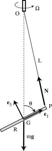
Figure 1: A hoop of center of mass G, attached to a wire OP, spins about the vertical axis OG, making a pitch angle $\theta$ with the vertical.

In this experiment, the angular rotation threshold being of order of a few rad/s, the wire can be simply spun with the fingers. Since it only requires a wire and a hoop, this experiment can be conveniently used as a classroom illustration of spontaneous symmetry breaking and bifurcation. Although the detail of the calculation is somewhat more subtle than that of the classical bead-on-a-hoop problem, since it deals with rigid body dynamics, the physics is basically the same and does not require the much heavier apparatus of the bead-on-a-hoop demonstration.

II Theory

II.1 Equation of motion

We consider a thin uniform hoop, of radius $R$ and mass $m$, fixed at a point P of its periphery by a massless wire of length $L\gg R$ (see figure 1). The wire is spun from its other end O at a constant angular velocity $\Omega$. The center of mass G is assumed to remain at the vertical of O. Let us first consider a torsionless wire, so that the hoop angular velocity $\dot{\phi}$ about the vertical axis ${\bf e}_{z}$ instantaneously follows the imposed angular velocity $\Omega$.

Let us consider the rotating frame of reference of the hoop $({\bf e}_{1},{\bf e}_{2},{\bf e}_{3})$. We note $\theta$ the pitch angle between the hoop plane and the vertical axis ${\bf e}_{z}$. We consider for simplicity a zero roll angle about ${\bf e}_{1}$ (i.e. we assume that the point P remains the highest point of the hoop), so that $\theta$ is the only degree of freedom for this problem. The absolute angular velocity $\omega$ of the hoop has two contributions. The first one, of magnitude $\Omega$, is imposed from O through the torsionless wire, and is about ${\bf e}_{z}=\cos\theta\,{\bf e}_{1}+\sin\theta\,{\bf e}_{3}$ (the points O and G are at rest, so that OG is the instantaneous axis of rotation when $\theta$ is kept constant). The second one comes from the pitch variation $\dot{\theta}$, and is about the axis ${\bf e}_{2}$. We therefore obtain

$$\mbox{\boldmath$\omega$}=\left(\begin{array}[]{l}\Omega\cos\theta\\ \dot{\theta}\\ \Omega\sin\theta\end{array}\right).$$ (1)

The potential energy is $V=mgz_{G}$, where $z_{G}\simeq R(1-\cos\theta)$ is the center of mass elevation to first order in $R/L$. The kinetic energy $T$ has two contributions: one from the rotation $\frac{1}{2}\mbox{\boldmath$\omega$}\cdot\tilde{I}\cdot\mbox{\boldmath$\omega$}$, where $\tilde{I}$ is the inertia matrix of the hoop relative to G, and one from the vertical translation of the center of mass, $\frac{1}{2}m\dot{z}_{G}^{2}\simeq\frac{1}{2}mR^{2}\dot{\theta}^{2}\sin^{2}\theta$. In the reference frame of the hoop, the inertia matrix $\tilde{I}$ has diagonal components $I_{1}=I_{2}=\frac{1}{2}mR^{2}$ and $I_{3}=mR^{2}$. The Lagrangian function ${\cal L}=T-V$ then finally writes

$${\cal L}=\frac{1}{4}mR^{2}\left[\Omega^{2}(1+\sin^{2}\theta)+\dot{\theta}^{2}(1+2\sin^{2}\theta)\right]+mgR\cos\theta.$$ (2)

Writing the Lagrange’s equation for the coordinate $\theta$, we end up with the differential equation of motion

$$\ddot{\theta}(1+2\sin^{2}\theta)-(\Omega^{2}-2\dot{\theta}^{2})\sin\theta\cos\theta+\Omega_{c}^{2}\sin\theta=0.$$ (3)

where $\Omega_{c}=\sqrt{2g/R}$.

This equation of motion can also be obtained from the angular momentum equation and Newton’s law. In the rotating frame of reference, the angular momentum equation reads

$$\frac{d{\bf L}}{dt}+\mbox{\boldmath$\omega$}{\times}{\bf L}={\bf\Gamma},$$ (4)

where ${\bf L}=\tilde{I}\mbox{\boldmath$\omega$}$ is the angular momentum and ${\bf\Gamma}={\bf GP}{\times}{\bf N}$ is the torque of the wire tension relative to the center of mass (the gravitational torque vanishes). The wire tension is obtained from Newton’s law,

$$m\ddot{z}_{G}\,{\bf e}_{z}={\bf N}+m{\bf g}.$$ (5)

To first order in $R/L$, ${\bf N}$ is vertical, so its torque is simply ${\bf\Gamma}\simeq-RN\sin\theta\,{\bf e}_{2}$. Using $z_{G}\simeq R(1-\cos\theta)$, we obtain

$${\bf\Gamma}\simeq-R\left(mg+mR(\dot{\theta}^{2}\cos\theta+\ddot{\theta}\sin\theta)\right)\sin\theta\,{\bf e}_{2}.$$ (6)

Replacing into (4) and projecting on ${\bf e}_{2}$, we finally recover the equation of motion (3).

II.2 Steady states and small oscillations

We are interested in the steady states and the natural frequency for small oscillations about them. To first order in $\theta$, equation (3) reduces to

$$\ddot{\theta}-\Omega^{2}\sin\theta\cos\theta+\Omega_{c}^{2}\sin\theta=0.$$ (7)

It is worth noting that this linearized equation is exactly the same as the one from the bead-in-a-hoop problem Siva . The difference between equations (3) and (7) originates from the kinetic energy of the center of mass translation, which is not present in the bead-on-a-hoop.

In addition to the trivial solution $\theta_{\mathrm{eq}}=0$, equation (7) has a non trivial solution for $\Omega\geq\Omega_{c}$,

$$\theta_{\mathrm{eq}}=\pm\cos^{-1}\left(\frac{\Omega_{c}}{\Omega}\right)^{2}.$$ (8)

Following the usual terminology, the pitch angle $\theta_{\mathrm{eq}}$ is the order parameter, and we introduce the reduced angular velocity $\epsilon=\Omega/\Omega_{c}-1$ as the control parameter. The linearization of (8) finally leads to the classical form of a supercritical pitchfork bifurcation for $\epsilon\ll 1$:

$$\theta_{\mathrm{eq}}\simeq 2\sqrt{\epsilon}.$$ (9)

Stability and natural frequency for small oscillations are obtained by introducing in equation (7) a small perturbation in the form

$$\theta(t)=\theta_{\mathrm{eq}}+\delta\theta\,e^{(\sigma+i\omega)t},$$ (10)

where $\theta_{\mathrm{eq}}$ stands for the trivial or non-trivial solution. The trivial solution is stable for $\Omega<\Omega_{c}$ ($\sigma=0$), with a natural frequency $\omega=(\Omega_{c}^{2}-\Omega^{2})^{1/2}$, and unstable for $\Omega>\Omega_{c}$, with a growth rate given by $\sigma=(\Omega^{2}-\Omega_{c}^{2})^{1/2}$ (and $\omega=0$). The non-trivial solution (8) is found to be always stable, with the same natural frequency. In terms of $\epsilon$, one can see that the period of the oscillations,

$$T\sim|\epsilon|^{-1/2},$$ (11)

diverges as one approaches the transition from both side. This critical slowing down is a usual signature of supercritical bifurcationDrazin .

II.3 Nonlinear oscillations

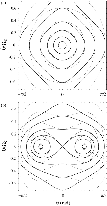
Figure 2: Orbits in the phase space $(\theta,\dot{\theta}/\Omega_{c})$ for the hula hoop (solid lines) compared to the bead-on-a-hoop system (dashed lines). ($a$): $\Omega=0.8\Omega_{c}$. ($b$): $\Omega=1.2\Omega_{c}$.

When the oscillation amplitudes about the steady states are not small, the nonlinear terms in (3) become important and may affect the dynamics of the system. The orbits in the phase space $(\theta,\dot{\theta})$ then provide a useful tool to characterize the nonlinear dynamics of the hula hoop, and to compare it with the one of the bead-on-a-hoop (7). The equation of motion can be integrated using the Painlevé invariant,

$$C=\dot{\theta}\frac{\partial\cal L}{\partial\dot{\theta}}-{\cal L},$$ (12)

which takes a constant value along an orbit (this invariant corresponds to the total energy $E=T+V$ in the case of a conservative system). Figure 2 shows isolines of $C$ for two forcing frequencies, below ($\Omega/\Omega_{c}=0.8$, fig. $a$) and above ($\Omega/\Omega_{c}=1.2$, fig. $b$) the transition, together with the orbits of the bead-on-a-hoop problem (dashed lines). One can clearly see from these phase portraits the trivial solution $\theta_{\mathrm{eq}}=0$ for $\Omega/\Omega_{c}=0.8$ and the two non trivial solutions (8) separated by a saddle point at $\theta=0$ for $\Omega/\Omega_{c}=1.2$. Note that we are only interested in the closed orbits in the domain $|\theta|\leq\pi/2$: orbits that cross $\theta=\pm\pi/2$ are not consistent with the assumption that the point P remains the highest point of the hoop.

Around the stable fixed points, both the two systems show nearly elliptic orbits, as expected from small harmonic oscillations. Larger oscillations of the hula hoop show orbits with sharper corners around $\theta\simeq 0$, associated to larger angular velocities $|\dot{\theta}|$. This discrepancy originates from the vertical translation of the center of mass, which is responsible for an additional pitch angle acceleration when the hoop is nearly vertical.

II.4 Timescales

Two timescales are relevant for a practical experiment: the startup timescale of rotation $\tau_{s}$ and the damping timescale of oscillations $\tau_{d}$. The startup timescale may be obtained considering the wire torsion. We start from an initially vertical hoop ($\theta=0$), and let now its rotation angle $\phi$ about ${\bf e}_{z}$ be free. The wire communicates a torque $\kappa(\phi-\Omega t)=\kappa\,\delta\phi$ to the hoop, where $\kappa$ is the torsion constant and $\delta\phi$ the wire torsion. The angular momentum equation about ${\bf e}_{z}$ applied to the hoop then reads

$$\frac{1}{2}mR^{2}\delta\ddot{\phi}+\kappa\,\delta\phi=0,$$ (13)

leading to a startup timescale $\tau_{s}\simeq R(m/2\kappa)^{1/2}$ (which corresponds also to the period of the wire torsion oscillations if no damping were present).

The damping timescale $\tau_{d}$ is relevant both for the $\phi$ oscillations due to the wire torsion, and for the $\theta$ oscillations around the equilibrium states. It can be obtained considering the dissipation with the surrounding air. With typical velocity of order m/s and hoop thickness $w$ of a few millimeters, we can make use of a turbulent estimate for the drag force. Neglecting $\dot{\theta}$ compared to $\dot{\phi}$, a unit length $dl$ of the hoop experiences a drag force $df\simeq\rho R^{2}\dot{\phi}^{2}w\,dl$, where $\rho$ is the air density. Integrating over the hoop perimeter leads to the frictional torque

$${\bf\Gamma}_{r}\simeq-\rho R^{4}\dot{\phi}^{2}w\,\frac{{\bf\Omega}}{|{\bf\Omega}|}.$$ (14)

The angular momentum equation about ${\bf e}_{z}$ reads

$$\ddot{\phi}+\left(\frac{\rho_{0}}{\rho}\frac{w}{R}\right)\dot{\phi}^{2}=0.$$ (15)

where $\rho_{0}$ is the hoop density. Taking $\dot{\phi}\simeq\Omega$ and $\ddot{\phi}\simeq\Omega/\tau_{d}$, the damping timescale finally writes

$$\tau_{d}\simeq\left(\frac{\rho_{0}}{\rho}\frac{w}{R}\right)\Omega^{-1}.$$ (16)

For values of practical interest, $\tau_{d}$ is of order of a few tens of the rotation period $\Omega^{-1}$. Note here that in the case of the real hula hoop game, the rolling friction on the player hips is fortunately dominant, leading to a damping timescale of order $\Omega^{-1}$.

III Experimental results

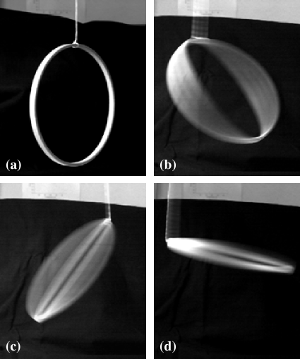
Figure 3: Pictures of the hoop. (a) The hoop at rest. (b) and (c) $\theta\simeq 37^{\mathrm{o}}$. (d) $\theta\simeq 78^{\mathrm{o}}$.

An experiment has been carried out using a wood hoop ($\rho_{0}\simeq 0.67$ g.cm^-3) of mass $m=15.5$ g, radius $R=86$ mm and section $4\times 10$ mm². The expected frequency threshold is then $\Omega_{c}/2\pi\simeq 2.40$ Hz (classical hula hoops have $\Omega_{c}/2\pi\simeq 1$ Hz). A simple cotton thread, of length $L=0.68$ m and mass less than 3% of the hoop mass, was fixed to a constant current motor. The startup timescale for this wire can be estimated from the free oscillation period, $\tau_{s}\simeq 5$ s (corresponding to a torsion constant $\kappa\simeq 2\times 10^{-6}$ N.m). This wire is far from being torsionless, and during the early stage of the rotation, torsional energy is stored into the wire. The wire progressively communicates rotation to the hoop, and the fluctations (due to a varying imposed rotation rate at its upper end, or to pitch angle variation at the other end) are smoothed down on a timescale $\tau_{d}$.

Seen from the side, the hoop rotation appears as Lissajous ellipses, whose principal axis makes an angle $\theta$ with the vertical axis. Pictures acquired from a simple CCD camera (see figure 3) allows us to easily measure the pitch angle $\theta$ within 1^o from these ellipses. The time aperture of the camera may blur the picture, but facilitate in some case the angle measurement (see for instance picture c).

Figure 4: Bifurcation diagram of the pitch angle $\theta$ as a function of the normalized angular velocity $\Omega/\Omega_{c}$. The solid line is the calculated solution (8), with $\Omega_{c}$ adjusted to fit the experimental data.

The measured pitch angles $\theta$, shown in figure 4, are in excellent agreement with the exact solution (8), except for low rotation rate, where non zero angles are measured below the expected transition. The experimental frequency threshold, obtained by extrapolating the curve down to $\theta\simeq 0$, is $\Omega_{c}/2\pi\simeq(2.30\pm 0.03)$ Hz, which agrees within 5% with the theoretical value. The discrepancy at low rotation rate is typical of an imperfect bifurcation, where small asymmetry in the apparatus (such as the position of the knot) slightly anticipates the destabilization of the basic state.

An interesting observation is that, for $\Omega\geq 2.6\Omega_{c}$ (see the dashed line in figure 4), the bifurcated state is no stable any more: a secondary instability appears, in the form of a slow precession of the center of mass, with a period of about ten rotation periods. This new behavior is probably an effect of the non zero mass of the wire, and can clearly not be described in our calculation, where the hoop center of mass is constrained to remain aligned with the vertical axis.

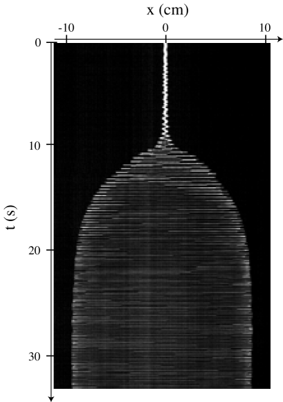
Figure 5: Spatio-temporal diagram of the light intensity recorded on an horizontal line, showing the wire oscillation, when the frequency $\Omega/2\pi$ is increased from 0 to 5.5 Hz.

Transient phenomena may also be investigated, by means of usual video processing. An illustration is given in figure 5, showing a spatio-temporal diagram obtained by collecting the light intensity recorded on a horizontal line passing through the wire. In this example, the imposed frequency $\Omega/2\pi$ has been suddenly increased from 0 to 5.5 Hz $\simeq 2.4~{}\Omega_{c}/2\pi$ (first arrow). One can see that, after a transient time of around 7 s (second arrow) during which the wire rotation propagates down to the hoop, the amplitude increases and saturates to a finite value.

Figure 6: Instantaneous pitch angle $\theta$ (left) and rotation frequency $\dot{\phi}/2\pi$ (right) as measured from figure 5. The origin time $t_{0}$ corresponds to the second arrow in that figure.

From this diagram, the instantaneous pitch angle as well as the instantaneous oscillation frequency $\dot{\phi}/2\pi$ may be extracted, as shown in figure 6. The frequency is obtained from averaging over 6 successive oscillations. Due to the progressive torsion of the wire, this frequency slowly approaches its imposed value 5.5 Hz. As a consequence, the increase of the pitch angle towards its stationary value $\theta_{\mathrm{eq}}\simeq 1.42$ rad is rather slow.

It is interesting to note that, when plotting the instantaneous pitch angle as a function of the instantaneous frequency (see figure 7), the bifurcation diagram of figure 4 is recovered to a high degree of accuracy. This suggests that the pitch angle follows ‘adiabatically’ the instantaneous frequency, so that the apparent growth rate is essentially controlled by the wire torsion more than the intrinsic dynamics of the instability (at least far from the transition).

Figure 7: Instantaneous pitch angle $\theta$ as a function of the instantaneous rotation frequency $\dot{\phi}/\Omega_{c}$ (same data as in figure 6). The solid line is the calculated solution (8), as in figure 4. The cross indicates the stationary solution $\theta_{\mathrm{eq}}\simeq 1.42$ rad for $\Omega=2.4~{}\Omega_{c}$.

IV Discussion

This simple experiment provides an interesting alternative to the bead-on-a-hoop Siva ; Fletcher ; Mancuso experiment as a mechanical analog to bifurcation and second-order phase transition in physics. The poor attention paid to the choice of the material and the experimental conditions illustrates the robustness of the phenomenon, and makes this experiment easy to work out by undergraduate students. Further experiments can be performed, e.g. studying the transient phenomena resulting from a small perturbation. As a suggestion, restrain the point P on the vertical axis when $\Omega>\Omega_{c}$ by means of a small hook around the wire. Releasing the hook allows us to measure the growth rate and to characterize its divergence as $\epsilon\rightarrow 0$. This method can be hardly achieved with a bead-on-a-hoop apparatus due to its inherent difficult access.

Another motion may compete with the bifurcation described in this paper: the hoop can rotate as a whole about the vertical axis, its center of mass remaining aligned with the wire. This is the usual motion for the conical pendulum, which also leads to a supercritical bifurcation with a threshold simply given by the natural frequency $\omega_{0}\simeq\sqrt{g/(L+R)}$. The conical pendulum motion overcomes the hula hoop motion for $\omega_{0}$ of order of $\Omega_{c}$, i.e. for a wire length of order of the hoop radius. Moving away the center of mass from the vertical axis may allow us to observe the competition between the two regimes, even for a longer wire.

Similar bifurcations as the result of a competition between centrifugal force and gravity are present in a number of situations. Spinning plates provides an interesting illustration: as for the real hula hoop, the motion here is forced by the precession of the rigid rod rather than its rotation. The imposed precession frequency has to overcome the natural frequency for the plate to stand up, and then the horizontal state is maintained by a parametric oscillation mechanism Caughey . Lasso roping is another example, where the rigid hoop is replaced by a deformable loop. Here again the motion is maintained by the precession of the spoke rather than rotation. As a consequence, the knot on the loop makes the spoke to rotate as well, so that the cord has to be continuously untwisted at its other end.

It is worth pointing out that this experiment can be carried out with any rigid body, not necessarily axisymmetric. In this case, the angle of the equilibrium state (8) remains unchanged, and the angular velocity threshold just becomes $\Omega_{c}=\sqrt{mga/(I_{3}-I_{1})}$, where $a=|{\bf GP}|$ is the distance between the center of mass and the knot. Note however that, for bodies with three different inertia moments, in addition to the bifurcation described here, inertial instabilities may also occur. Such instability involves the roll angle about ${\bf e}_{1}$ as an additional degree of freedom, and is not described by our calculation.

- (1) Donald T. Greenwood, Principles of dynamics (Prentice-Hall, Englewood Cliffs, NJ, 1988), 2nd ed., Sec. 8.
- (2) H. Keith Moffatt, “Spinning eggs — a paradox resolved,” Nature 416, 385–386 (2002).
- (3) Philip G. Drazin, Nonlinear systems (Cambridge University Press, Trumpington Street, Cambridge CB2 1RP, 1992), pp. 1–48.
- (4) Jean Sivardière, “A simple mechanical model exhibiting a spontaneous symmetry breaking,” Am. J. Phys. 51 (11), 1016 (1983).
- (5) Glenn Fletcher, “A mechanical analog of first- and second-order phase transitions,” Am. J. Phys. 65 (1), 74 (1997).
- (6) Richard V. Mancuso, “A working mechanical model for first- and second-order phase transitions and the cusp catastrophe,” Am. J. Phys. 68 (3), 271 (2000).
- (7) Thomas K. Caughey, “Hula-Hoop: An Example of Heteroparametric Excitation,” Am. J. Phys. 28, 104–109 (1960).