Model Flames in the Boussinesq Limit: The Effects of Feedback

Abstract

We have studied the fully nonlinear behavior of pre-mixed flames in a gravitationally stratified medium, subject to the Boussinesq approximation. Key results include the establishment of criterion for when such flames propagate as simple planar flames; elucidation of scaling laws for the effective flame speed; and a study of the stability properties of these flames. The simplicity of some of our scaling results suggests that analytical work may further advance our understandings of buoyant flames.

I Introduction

In several areas of research, the feedback of a propagating diffusive (pre-mixed combustion) flame on a fluid, and the consequent effects of the flame itself, is of considerable interest. In the astrophysical context, for example, the speedup of nuclear reaction fronts of this type in the interior of white dwarf stars is thought to be one possible way that such stars undergo thermonuclear disruption, e.g., a Type Ia supernova (cf. Whelan73 ; Livne93 ; Khokhlov95 ; Niemeyer95 ; Reinecke99 ; Gamezo02 ). Much of the literature on this subject has focused on the speedup of such flames for prescribed flows, and substantial advances have been made in this regard recently Constantin00 ; this is the “kinematic” problem, in which one seeks to establish rigorous limits on flame speedup in the case in which there is no feedback onto the flow. The aim of this paper is to study the simplest case of feedback, namely that which occurs when a flame propagates vertically, against the direction of gravity. As described extensively in the previously cited literature, it is generally believed that under such circumstances, the flame front is likely to become distorted by the action of the Rayleigh-Taylor instability, and thus achieves speedup; these calculations have been largely illustrative, and based upon simulations using fully-compressible fluid dynamics (e.g., Ropke02 ) and fairly realistic nuclear reaction networks.

Here, we focus on a much simpler problem; we study such flames in the Boussinesq limit (leading to a far simpler computational problem) and for highly simplified reaction terms (avoiding the complexities of realistic nuclear reaction networks). In this way, we are able to isolate the various effects which lead to flame speedup, which is particularly important if one is to connect such simulations to the extant analytical work on this subject (e.g., Audoly00 ; Berestycki02 ; Constantin00 ). Indeed, an important motivation for this work is to elucidate simple scaling laws — if they exist — in order to suggest further analytical studies.

Our paper is structured as follows: In the next section, we describe the specific physical problem we wish to study, establish the equations to be solved, and describe the method of solution. In §III, we present our results, and in §IV, we provide a summary and discussion.

II The Problem

The effect of gravity on the temperature distribution in a reacting incompressible fluid with thermal diffusivity $\kappa$, viscosity $\mu$, and density $\rho$ can be described by the set of Navier-Stokes and advection-diffusion-reaction equations,

$$\rho\left[\frac{\partial{\bf v}}{\partial t}+({\bf v}\cdot\nabla){\bf v}\right] = -\nabla p+\mu\nabla^{2}{\bf v}+\rho{\bf g},$$

$$\frac{\partial T}{\partial t}+{\bf v}\cdot\nabla T = \kappa\nabla^{2}T+R(T),$$ (1)

$$\nabla\cdot{\bf v} = 0,$$

where ${\bf v}$ is the fluid velocity and, without loss of generality, the temperature $T$ has been normalized to satisfy $0\leq T\leq 1$. The thermal diffusivity and viscosity are assumed to be temperature-independent, and density variations are assumed to be small enough to be described by the Boussinesq model, e.g., $\rho(T)=\rho_{\circ}+(\Delta\rho/\rho_{\circ})T$. The model (1) can be derived from a more complete system under the assumption of unity Lewis number ${\rm Le}$ (the ratio of thermal and material diffusivities), and this article addresses only the ${\rm Le}=1$ case.

The Boussinesq model is the simplest system exibiting buoyancy effects (and thus allowing for feedback to the flame) without introducing the complexities associated with the presence of sound wave and stratification of background “atmosphere”. Because our intentions is to elucidate basic priciples, rather than realistically modeling specific physical situations, we view our approach as sufficient for the chosen task.

We consider a reaction term of Kolmogorov-Petrovskii-Piskunov (KPP) type KPP , of the form

$$R(T)=\alpha T(1-T)/4\,,$$ (2)

where $\alpha$ is the (laminar) reaction rate. This reaction form has an unstable fixed point at $T=0$, the “unburned” state, and a stable one at $T=1$, the “burned” state. Thus a fluid element with positive temperature will inevitably evolve to the burned state in a characteristic time of order $1/\alpha$. As is well-known from the combustion literature, the temperature equation from the system above admits — for a stationary fluid, and in the absence of gravity — one-dimensional solutions in the form of burning fronts propagating with laminar burning speed $s_{\circ}$, and with characteristic flame thickness $\delta$,

$$s_{\circ}=\sqrt{\alpha\kappa}\,,\hskip 28.45274pt\delta=\sqrt{\alpha/\kappa}\,.$$ (3)

If it is further assumed that $T\rightarrow 1$ as $y\rightarrow-\infty$, and $T\rightarrow 0$ as $y\rightarrow+\infty$, then the front propagation is in the positive $y$ direction.

It is convenient to adopt the front thickness $\delta$ and the inverse reaction rate $\alpha^{-1}$ as the units of distance and time respectively. In these units the problem control parameters are the Prandtl number ${\rm{Pr}}$ and the non-dimensional gravity $G$,

$${\rm{Pr}}=\frac{\nu}{\kappa}\,,\hskip 28.45274ptG=g\,\left(\frac{\Delta\rho}{\rho_{\circ}}\right)\frac{\delta}{s_{\circ}^{2}}\,,$$ (4)

where $\nu$ is a kinematic viscosity $\nu=\mu/\rho_{\circ}$. In addition, the system is characterized by a number of length scales specifying the initial state, which are in our case the dimensionless amplitude $A$ and the dimensionless wavelength $L$ of the initial flame front perturbation, $f(x)=a\cos({2\pi x}/{l})$,

$$A=a/\delta\,,\hskip 28.45274ptL=l/\delta\,.$$ (5)

The vertical size of the computational domain was kept large so as to avoid effects due to the upper and lower walls of the computational box; in all cases, we have verified that such artifacts are not present. For this reason, the box height does not enter as a problem parameter. The initial velocities are set to zero, and most computations were carried out for ${\rm{Pr}}=1$. A typical initial state of our flame calculation is shown in Fig. 1.

Figure 1: A typical initial state of a flame calculation.

Because we focus on the two-dimensional problem, it is convenient to re-write Eqns. (1) in the stream function and vorticity formulation in dimensionless form,

$$\frac{\partial\omega}{\partial t}=\;-{\bf v}\cdot\nabla\omega\;+\;{\rm{Pr}}\nabla^{2}\omega\;-\;G\frac{\partial T}{\partial x}\,,$$ (6a)

$$\frac{\partial T}{\partial t}=-{\bf v}\cdot\nabla T+\nabla^{2}T+\frac{1}{4}T(1-T)\,,$$ (6b)

using $\delta$ and $\delta/s_{\circ}$ as units of length and time respectively. Here ${\bf v}$ is the non-dimensional velocity and $\omega$ is the non-dimensional vorticity ($\omega\equiv\nabla\times{\bf v}=\nabla^{2}\psi$). We solve the system (Eqns. 6) numerically. The solution is advanced in time as follows: a third order Adams-Bashforth integration in time advances $\omega$ and $T$, where spatial derivatives of $\omega$ and $T$ are approximated by fourth-order (explicit) finite differences. The subsequent elliptic equation for $\psi$ is then solved by the bi-conjugate gradient method with stabilization, using the AZTEC library AZTEC . Finally we take derivatives of $\psi$ to update ${\bf v}$.

The resolution of the simulations was chosen to fully resolve the laminar flame structure. For the KPP reaction term (2), the laminar flame thickness is approximately $12\,\delta$, and the grid spacing $\Delta x=\Delta y=1$ (in the units of $\delta$) was used in most of the computations. The laminar flame speed computed at this resolution agrees with the theoretical value to within 1%. This corresponds to at least $16$ zones per wavelength (of the initial perturbation) which is sufficient to resolve the flow. Most of the computations were executed on a domain half the width of the initial perturbation wavelength, and reflecting boundary conditions were applied.

Simulation times of $t=200$ – $500$ (in units of $\delta/v_{\circ}$) were required to measure the bulk burning rate, on computational grids ranging from $8\times 256$ for $L=16$ to $64\times 2048$ for $L=128$. Larger domains were necessary to obtain velocity fields (e.g. $64\times 3072$ for $L=128$), to avoid the influence of boundary conditions at the top and bottom. Fortunately, only the velocity in the reaction region affects the shape of the flame front and, consequently, the bulk burning rate, so slight errors in estimating velocities far away from the front due to upper and lower boundaries do not affect our results. The comparison with linear analysis was done using the same resolution and domain sizes up to $512\times 4096$.

By its nature, this study was comprised of a large number ($\sim 250$) of simulations each representing a data point, as opposed to a close examination of just a few simulations as in a case-study approach. Confidence in the numerical accuracy was gained at the cost of a small number of additional test simulations. Some simulations were repeated using lower and higher resolutions, domains of different sizes in vertical direction, and with several wavelengths across the width of the domain. Special attention was devoted to simulations with different Prandtl numbers, to ensure that both diffusive and viscous scales were resolved.

Finally, a comment regarding the two-dimensional nature of our simulations. In a recent study of the closely related Rayleigh-Taylor instability Young01 , Young et al. specifically compared the behavior of fingering and mixing in two- and three-dimensional flows, with the result that while the specifics, e.g., finger growth rates, were quite sensitive to dimensionality, the phenomenology nevertheless turned out to be rather similar. Flames do however introduce a very useful physical simplification into the Rayleigh-Taylor problem: Because flames consume all density features at the flame front with scales smaller than the flame thickness, the Rayleigh-Taylor problem is “regularized” by the burning process even in the limit of vanishing viscosity. For this reason, a key difference between 2-D and 3-D – namely, the difference between small-scale turbulent structures in two and three dimensions – is sharply reduced in the burning case. The remaining difference between 2-D and 3-D is then mostly related to the difference in propagation speed between buoyant parallel rolls (the 2-D case) and buoyant tori (the 3-D case), with tori propagation more quickly, i.e., we would expect 3-D flames to propagate more quickly than 2-D flames, all other things being equal. We plan to explore this point in future three-dimensional studies of flame propagation.

III Results

In this section, we discuss the results of our calculations, focusing successively on the bulk burning rate, the evolution of the burning travelling front, and the ultimate transition to a travelling (burning) wave. Our central interest is in disentangling the dependence of the flame behavior on the key control parameters of the problem.

III.1 Travelling wave flame

For a wide range of parameters, we were able to construct a sufficiently large computational domain that we could observe travelling waves of the temperature distribution, propagating with constant speed. Depending on simulation parameters, the initial perturbation either damps (e.g., the flame front flattens) or forms a curved front. The flat front moves in the motion-free (in the Boussinesq limit) fluid, has laminar front structure, and propagates with the laminar front speed.

Figure 2: Travelling wave isotherms ($T=0.1$ and $T=0.9$) and streamlines for two system with different simulation parameters. Note that the system on the right has been rescaled by a factor of $1/4$ both horizontally and vertically.

The typical curved front is shown in Fig. 2; it has the wavelength of the initial perturbation and is characterized by narrow dips (lower apexes), where the cold fluid falls into the hot region, and by wide tips (upper apexes), where buoyant hot fluid rises into the cold fluid. In the initial stages, the evolution pattern is similar to bubble and spike formation during the Rayleigh-Taylor instability Chandrasekhar61 ; Landau87 ; in later stages, small scale structures are consumed by the flame, and, finally, the flame evolves toward the travelling wave solution shown in Fig. 2. The shape of the stable front is determined by gravity, $G$, and wavelength, $L$, and can be characterized by two vertical length scales associated with the spatial temperature variation ($h_{T}$) and the spatial velocity variation ($h_{V}$) of the flame. The speed of the curved front is always higher than the laminar flame speed, because of the increase in the flame front area and transport. Finally, we notice that the streamlines in Fig. 2 indicate that the flow underlying the propagating flame is characterized by rolls propagating upward.

One of our primary interests is to quantify the effects of variations in wavelength and gravity on the flame speed. It is convenient to define the speed of the travelling wave flame by the bulk burning rate Constantin00 ,

$$s(t)=\frac{1}{l}\int^{l}_{0}\frac{\partial T(x,y,t)}{\partial t}~{}dx~{}dy\,;$$ (7)

this definition has the considerable advantage that it reduces to the standard definition of the flame speed when the flame is well-defined, and it is accurate to measure even for cases where the burning front itself is not well-defined. Henceforth we refer to it simply as the flame speed.

Figure 3: Bulk burning rate (travelling wave speed) $s$ as function of wavelength $L$ for different values of gravity $G$.

Our first result (shown in Fig. 3) is that the flame speed increases with wavelength $L$ and with the gravitational acceleration $G$, and is independent of the initial perturbation amplitude $A$. More specifically, the flame becomes planar and moves at the laminar speed ($s=s_{\circ}$) if $G$ is smaller than some critical value ${G_{\rm cr}}$; if $G$ lies above this critical value, the flame speed can be fit by the expression,

$$s=s_{\circ}\sqrt{1+k_{1}(G-G_{1})L}\,,$$ (8)

where $k_{1}\approx 0.0486$ is obtained from measurements derived from the simulation data. The second tuning parameter, $G_{1}$, was found to be a function of the perturbation wavelength (Fig. 4), $G_{1}=8(2\pi/L)^{1.72}$. For a relatively wide range of parameters, Eq. (8) describes experimental data well, but must be applied with caution near the cusp at $G=G_{1}$ shown in Fig. 3. Roughly speaking, this cusp can be interpreted as the transition between the planar and curved flame regimes, $G_{1}\approx{G_{\rm cr}}$; closer investigation of the transition region shows that ${G_{\rm cr}}<G_{1}$, and that the fit (Eq. 8) underestimates the flame speed in this transition region (Fig. 5).

Figure 4: Transitional point $G_{1}$ as a function of wavelength.

Figure 5: Amplitude of the stable front as function of gravity for the wavelength $L=32$. The scaling relations shown here are discussed in the text.

The behavior near the transition is discussed in detail in the theoretical work carried out by Berestycki, Kamin & Sivashinsky Berestycki02 . They derive the one-dimensional evolution equation for the front interface $y(x)$ and prove mathematically the following properties of $y(x)$, relevant to our case: (1) the existence of ${G_{\rm cr}}\sim(2\pi/L)^{2}$ such that there is no nontrivial solution for $G<{G_{\rm cr}}$ (i.e. the front is flat for $G<{G_{\rm cr}}$); (2) the existence of ${G_{\rm cr}}^{*}=4{G_{\rm cr}}$ such that for $G>{G_{\rm cr}}^{*}$ there are two symmetrical (curved) solutions $y^{+}(x)$ and $y^{-}(x)$ which are stable, and any other solution including the trivial is unstable; (3) metastability of any solution except $y^{+}(x)$ and $y^{-}(x)$ in the range ${G_{\rm cr}}<G<{G_{\rm cr}}^{*}$, and convergence of this metastable solution to either $y^{+}(x)$ or $y^{-}(x)$. Also, based on the derivation in Berestycki02 , it can be shown that the flame speed in the metastable regime scales as follows Kiselev ,

$$(s/s_{\circ}-1)\propto(G-{G_{\rm cr}})^{2}~{}~{}{\rm as}~{}~{}(G-{G_{\rm cr}})\rightarrow 0\,.$$ (9)

Our simulations confirm the dramatic increase of stabilization times close to the critical gravity value ${G_{\rm cr}}$. For this reason, it is very difficult to obtain reliable results regarding the flame speed in this transition regime. Even detecting the critical point takes significant computational effort (Fig. 5); measuring the velocity, which in this parameter regime differs from $s_{\circ}$ by a very small amount, is harder still.

However, the transition is sharper and is easier to see when studying the vertical distance between the upper and lower apexes of the flame, $h_{T}$, measured by the expression,

$$h_{T}=\int_{-\infty}^{\infty}\left(T(0)-T(l/2)\right)dy\,.$$ (10)

In the limit of large wavelengths ($L\gg 1$), the transition occurs at small values of gravity, and the flame speed is determined by a single parameter, the product $LG$. If, in addition, the product $LG$ is large, the flame speed scales as $s/s_{\circ}\approx 0.22\sqrt{LG}$. This result is in good agreement with the rising bubble model Bychkov00 which, in the Boussinesq limit, predicts $s/s_{\circ}=\sqrt{LG/6\pi}\approx 0.23\sqrt{LG}$ for a 2-D open bubble Layzer55 . We further observe that in the large wavelength limit, the $h_{T}/l$ ratio obeys the same scaling (Fig. 5).

We note that the flame structure shares features of flame propagation from both shear and cellular flow. For instance, the temperature distribution closely resembles that of a flame distorted by a shear flow, while the velocity distribution resembles that inside an infinitely tall cell. The flame speed in the shear and cellular flow is determined by the flow speed and by the length scale of the flow (period of shear or cell size) Vladimirova03 . In particular, in both cases the flow speed scales with maximum flow velocity as $s\propto v_{max}^{n}$, with $n=1$ for burning in the shear flow and $n=1/4$ for burning in the cellular flow. Similarly, we have tried to determine whether the flame speed relates to the maximum velocity of the flow when flow and flame are coupled through the Boussinesq model. The available data (shown in Fig. 6) do not demonstrate a power law dependence with a single well-defined power. Furthermore, the dependence on $L$ is not as dramatic as in the cases of shear or cellular flows.

Figure 6: The flame speed as function of maximal flow velocity.

III.2 The thin front limit

The thin front limit is particularly important for developing models of flame behavior. For many applications — especially in astrophysics — resolving flames (by direct simulation) is prohibitively expensive, and understanding flame propagation in the limit in which the flame front becomes indefinitely thin (when compared to other length scales of the application) is critical for designing flame models. Of course, this same limit is of intrinsic mathematical interest.

Particularly important is the dependence of the flame speed on the wavelength of the front perturbation in the thin front limit. We have already pointed out that instabilities with larger wavelengths have higher travelling wave speeds, so that eventually the instability with the largest wavelength allowed by the system dominates. (In our non-dimensionalization, this is the instability with the highest ratio of wavelength to laminar front width).

In this context, it is convenient to switch from our “laminar flame units” to the so-called “G-equation units”. The G-equation is a model for reactive systems where very low thermal diffusivity is exactly balanced by high reaction rate (see e.g., Pelce88 ). The diffusion and reaction terms in the temperature equation are replaced by a term proportional to the temperature gradient,

$$\frac{\partial T}{\partial t}+{\bf v}\cdot\nabla T=s_{\circ}|\nabla T|\,,$$

so that the front propagates normal to itself at the laminar flame speed $s_{\circ}$. The Boussinesq fluid model, combined with the G-equation flame model, has the following physical parameters: (1) flow length scale $l$, (2) laminar flame speed $s_{\circ}$, (3) gravity $g$, and (4) fluid viscosity $\nu$. Choosing $l$ and $l/s_{\circ}$ as the length and time units, the governing non-dimensional parameters are $\tilde{g}=gl/s_{\circ}^{2}$ and $\tilde{\nu}=\nu/ls_{\circ}$; the corresponding parameters in the laminar flame unit system are $\tilde{g}=LG$ and $\tilde{\nu}={\rm{Pr}}/L$. Note that in the limit $L\rightarrow\infty$ while keeping ${\rm{Pr}}=1$, the Navier-Stokes equation becomes the Euler equation and $\tilde{\nu}\rightarrow 0$, leaving only one parameter in the system, $\tilde{g}=(\Delta\rho/\rho_{\circ})gl/s_{\circ}^{2}=LG$.

Table 1: Three simulations with $LG=32$ discussed in the text.

setup	$L$	$G$	$s/s_{\circ}$	$h_{T}/l$	$v_{\rm max}/s_{\circ}$
(a)	32	1	1.34	0.98	4.40
(b)	128	1/4	1.51	0.83	5.06
(c)	256	1/8	1.57	0.75	5.01

In our simulations ${\rm{Pr}}=1$, so it is not surprising that for large $L$, almost all aspects of the system are well characterized by the $LG$ product alone. For example, the formula for the bulk burning rate, $s/s_{\circ}=\sqrt{1+k_{1}LG}$ for $G>G_{1}$ well describes our experimental results. Next, consider the travelling wave solutions shown in Fig. 2; these two systems have the same $LG$ product, with $L=32$ and $L=128$, and move at the speed $s/s_{\circ}=1.34$ and $s/s_{\circ}=1.51$ respectively. The wavelength here is comparable to the laminar front thickness (indicated by the two limiting isotherms $T=0.1$ and $T=0.9$). Still, the front shape as well as flame speed and fluid velocities are very similar.

Figure 7: Travelling wave solution for two systems with $LG=32$, with $L=128$ (dashed lines), and with $L=256$ (solid lines). The isotherms $T=0.1$ and $T=0.9$ are shown in the middle panel. The top panel shows the temperature profiles and vertical velocities (along $\bf{g}$) at $x=0.5$ (upper flame front apex); the bottom panel plot shows the same things at $x=0$ (lower flame front apex).

One can see similarity more clearly in Fig. 7 (middle panel), which compares systems with $L=128$ and $L=256$. The agreement between bulk burning rates is very good ($s/s_{\circ}=1.51$ and $s/s_{\circ}=1.57$). The match between the two integral measures $h_{T}$ is weaker ($h_{T}/l=0.83$ and $h_{T}/l=0.75$), suggesting that the systems in consideration are still far from the infinitely thin front limit, but this is apparent from the distance between limiting isotherms. We have also compared the temperature and velocity profiles at the upper and lower apexes of the flame (Fig. 7, the top and the bottom panels). The velocity is — as expected — essentially zero well ahead of the temperature front, but significant motion extends far behind it; the absolute maximum velocity is located in the vicinity of the lower apex and is related to the bulk burning rate (Fig. 6). By examing the detailed velocity profiles we find that velocities at the flame front also obey the $LG$ product scaling and, together with the temperature distribution, determine the bulk burning rate. However, the velocities well behind the front can be quite different for two systems with the same $LG$ product (cf. Fig. 2).

Finally, consider the temperature during the instability growth phase, shown for three different cases (with $LG=512$) in Fig. 8. Although the wavelength to laminar front thickness ratio affects small scale features, we again clearly see the similarity scaling connecting these solutions.

Figure 8: The isotherm $T=0.5$ during the instability growth phase, shown for three systems with $LG=512$ but different $L$ (top: $L=64$, middle: $L=128$, bottom: $L=256$). The initial amplitude is $a/l=1/8$, and snapshots are taken at times $t(s_{\circ}/l)=0,\,1/16,\,2/16,\,3/16,\,4/16\,.$

As we have shown above, the dependence on a single parameter, namely the $LG$ product, in the infinitely thin front limit follows from dimensional analysis; and for reasonably thin fronts, we were able to confirm the $LG$ product scaling. At the same time, we noticed that the length of the velocity variation, $h_{V}$, does not scale with $LG\equiv\tilde{g}$. It is reasonable to assume that $h_{V}$ is controlled by the other parameter, namely, the non-dimensional viscosity $\tilde{\nu}={\rm{Pr}}/L$, which is essentially zero in the thin flame limit. One can understand this as follows.

From Eq. (6a), we can see that vorticity is generated in the regions with significant temperature gradients, e.g., on the scale $h_{T}$, and is advected by the flow on spatial scales of order $h_{V}$. Thus, positive vorticity is generated in the domains $nl<x<(n+1/2)l$, while negative vorticity is generated in the domains $(n+1/2)l<x<(n+1)l$; however, the total (signed) vorticity in the domain is conserved. Diffusion of vorticity occurs predominantly across the boundaries $x=nl/2$. More directly, it is straightforward to integrate the vorticity equation (Eq. 6a) over the area $nl<x<(n+1/2)l$ to obtain the vorticity balance,

$$\dot{\Omega} = \tilde{g}s_{\circ}^{2}\frac{h_{T}}{l}=$$

$$= \tilde{\nu}s_{\circ}^{2}\int_{-\infty}^{\infty}\left[\frac{\partial^{2}\tilde{v}_{y}}{\partial\tilde{x}^{2}}\right]_{\tilde{x}=0}+\left[\frac{\partial^{2}\tilde{v}_{y}}{\partial\tilde{x}^{2}}\right]_{\tilde{x}=1/2}d\tilde{y}\,.$$

Here $\dot{\Omega}$ is the total vorticity generated in the roll $nl<x<(n+1/2)l$, and diffused through its boundaries. In Fig. 9 we have plotted the non-dimensional vorticity generation, averaged in the area element $(l/2,\Delta y)$, $\tilde{f}_{\omega}=\tilde{g}(l/s_{\circ}^{2})(\Delta\dot{\Omega}/\Delta y)$, and corresponding fluxes across the roll boundaries. Note that only diffusion can lead to vorticity transport across roll boundaries because the transverse flow vanishes identically at the separatrices.

Figure 9: Vorticity generation in the roll (solid line) and vorticity fluxes through the separatrices between the rolls (dashed line), as a function of height $y$ for a flame with $L=32$ and $G=1$ (top panel) and for a flame with $L=128$ and $G=1/4$ (bottom panel). The areas below the solid and dashed lines are equal to $h_{T}/l$.

In other words, in the thin flame limit, vorticity generation depends on the $LG$ product, but not on the viscosity; however, in steady state, we know that vorticity generation and destruction must balance exactly. Since the vorticity destruction depends on the diffusion term ${\rm{Pr}}\nabla^{2}\omega$, which decreases as $L$ increases, balance can only be achieved if the length of the vorticity diffusion region (i.e. the separatrix separating adjacent rolls) lengthens. Thus, we expect $h_{V}$ to scale inversely with $\tilde{\nu}={\rm{Pr}}/L$. Indeed, we expect $h_{V}\rightarrow\infty$ as ${\rm{Pr}}\rightarrow 0$.

III.3 Comparison with linear stability analyses

A thorough analysis of the linear behavior of our system was presented by Zeldovich et al. Zeldovich85 ; in this subsection, we compare our results with theirs.

The simplest case studied is the so-called Landau-Darrieus instability, in which the flame is considered as a simple gas dynamic discontinuity Darries38 ; Landau44 . The fluid on either side of the discontinuity is assumed to obey the Euler equation; the fluid is assumed to be incompressible; there is no temperature evolution equation; and the front is assumed to move normal to itself with a given laminar speed. The important parameter is the degree of thermal expansion, $\theta\equiv\rho_{\rm fuel}/\rho_{\rm ash}$, across the flame front. The resulting instability growth rate is proportional to the product of the laminar flame speed and the wavenumber of the front perturbation, with a coefficient of proportionality depending on $\theta$. For $\theta=1$, which corresponds to the Boussinesq limit, the growth rate is identically equal to zero.

The Landau-Darrieus model is however not valid for wavelengths short compared to the flame thickness, for which it predicts the largest growth rate; this deficiency was resolved by Markstein Markstein64 , who introduced an empirical “curvature correction” for the flame speed within the context of the Landau-Darrieus model. One consequence of this correction is that the instability is suppressed for wavelengths shorter than a specific critical cutoff wavelength, while for wavelengths much larger than this cutoff lengthscale the growth rate approaches zero as $1/L$, just as in the Landau-Darrieus model.

Figure 10: Growth exponent for a single mode and two initial amplitudes $A\equiv a/\delta=4$ and $A=8$. The dimensionless wavelengths are $L\equiv l/\delta=512$ (dashed) and $L=1024$ (solid). The dotted lines correspond to the linear stability analysis prediction, Eq.(13).

Gravity can be introduced in this type of model in a very similar way, as shown by Zeldovich et al. Zeldovich85 . Rewriting their result in our notation, and taking into account $\theta=1$ and ${\rm{Le}}=1$ (which leads to the Markstein curvature correction constant being set equal to unity), we can reduce their final result to the following expression for the growth rate,

$$\gamma=\frac{s_{\circ}}{2\delta}k\left[\sqrt{1+k(k-2)+2G/k}-1-k\,\right],$$ (11)

where $k=2\pi/L$. A more elaborate model for the flame, introduced by Pelcé & Clavin Pelce82 , avoids the empirical curvature correction constant and, in the Boussinesq limit, gives the growth rate expression

$$\gamma=\frac{s_{\circ}}{2\delta}k\left[\sqrt{1+2G/k}-1-k-\frac{k}{\sqrt{1+2G/k}}\right]\,.$$ (12)

In the limit of thin fronts, $L\gg 1$, both models reduce to the same expression, which also recovers the $LG$ similarity scaling already discussed above,

$$\gamma\frac{l}{s_{\circ}}=\pi\left(\sqrt{1+\frac{1}{\pi}LG}-1\right).$$ (13)

To compare our calculations with this result, we have computed the growth rate for a single wavelength for a system with $L=512$ and $L=1024$ (see Fig. 10). The growth rates predicted by Eq.(13) are shown as horizontal dotted lines for each $LG$ product. An ideal system in the linear regime would have a constant growth rate; in our simulations we observe an essentially time-independent growth rate only after some transitional period, $t<0.1\,l/s_{\circ}$, and before the flame stabilization time, which depends on parameters. The transitional period at the beginning of our simulations can be explained by artificial initial conditions, e.g. zero velocity and prescribed temperature profile across interface. The decrease in the growth rate at later times is related to the stabilization of the flame front. Naturally, the faster-growing instabilities with higher $LG$ product and the systems starting with larger initial amplitudes reach the steady-state more quickly. In addition, we observe the influence of the finite flame thickness — plots with $L=1024$ approache closer to the infinitely thin limit than plots with $L=512$. But in spite of the finite flame thickness and non-zero viscosity, one can clearly see the similarity scaling on $LG$ and good agreement with theory (Fig. 11).

Figure 11: Growth exponent for a single mode measured at the maximum for $A=4$ and $L=1024$. The solid line corresponds to the linear stability analysis prediction, Eq.(13).

In order to obtain the stability condition, we set $\gamma=0$ in the expressions (11) and (12), and obtain

$$G_{\rm cr}=2k^{2}\,$$ (14)

for the Markstein model, and

$$G_{\rm cr}=\frac{k}{2}\left[\frac{1}{4}\left(1+k+\sqrt{(1+k)^{2}+4k}\right)^{2}-1\right]$$ (15)

for the Pelcé and Clavin model. We emphasize that both of these models assume an inviscid fluid, while viscosity is present in our simulations. In Fig. 12 critical gravities derived using both models are plotted next to numerical simulations data for different Prandtl numbers.

Similarly, we can consider the relation between the instability growth rate and the amplitude of the stable flame front, using the assumption that the flame front is composed of joined parabolic segments whose amplitude is small when compared to their wavelength Zeldovich85 . The resulting estimate depends on the growth rate, Eq. (13),

$$\frac{h_{T}}{l}=\frac{1}{8}\;\left(\gamma\frac{l}{s_{\circ}}\right)\,,$$

Comparing the result with the fit derived from the experimental data shown in Fig. 5 we notice that, in the thin front limit and for values of $G$ larger than critical, both numerical experiment and theoretical model predict $h_{T}/l\approx 0.22\sqrt{LG}$.

Figure 12: Critical gravity ${G_{\rm cr}}$ for different values of ${\rm{Pr}}=\nu/\kappa$. Our results are fit with power laws, in the form ${G_{\rm cr}}=C(2\pi/L)^{n}$, with measured values of $n=2.68$, $C=43.94$ for ${\rm{Pr}}=4$; $n=2.01$, $C=10.31$ for ${\rm{Pr}}=1$; and $n=1.73$, $C=6.21$ for ${\rm{Pr}}=1/4$. The two solid lines are provided by inviscid theory (${\rm{Pr}}=0$), corresponding to the Markstein and the Pelcé & Clavin models.

Finally, we note that a quick comparison of the asymptotic behavior of the Rayleigh-Taylor Chandrasekhar61 ; Landau87 and Landau-Darrieus Darries38 ; Landau44 instabilities for large $L$ gives $\gamma\propto L^{-1/2}$ for Rayleigh-Taylor and $\gamma\propto L^{-1}$ for Landau-Darrieus. In our Boussinesq case, the same asymptotic limit gives $\gamma\propto L^{-1/2}$: the instability behaves like the Rayleigh-Taylor instability at long wavelengths, i.e., longer wavelengths grow more slowly, but saturate later and reach larger front speeds.

III.4 Transition to the travelling wave

The transition time during which the temperature front is formed is of the order of the laminar burning time across the period, $0.5\,l/s_{\circ}$, but a much longer time is needed to stabilize the velocity pattern behind this front. Fig. 8 illustrates the process for a moderate value of $L$; in Fig. 13 we show snapshots for a flame with an $L$ value closer to the Rayleigh-Taylor limit just discussed. Indeed, Fig. 13 shows morphology strongly reminiscent of the Rayleigh-Taylor instability, namely upward-moving “bubbles” and downward moving “spikes”. As mentioned earlier, the reaction stabilizes the shape of the moving front, and eventually the flame interface will become smooth, similar to those shown in Fig. 2. The typical flame stabilization time is of the order of $L/s_{\circ}$, provided the initial perturbation amplitude is large enough (on the order of a fraction of $L$). During the transition, the system with larger $L/\delta$ ratio develops more complicated structures (compare Fig. 13 with Fig. 8) — the details on the scale of flame thickness and smaller are consumed by the burning. A similar effect is observed in the Rayleigh-Taylor instability on the dissipation scale, but due to viscosity and diffusion rather than burning.

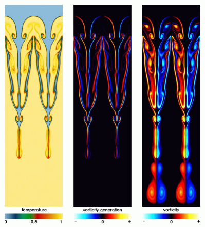
Figure 13: The temperature, vorticity generation rate, and vorticity (from left to right) for the system with $L=256$ and $G=4$ at time $t=72\,\delta/s_{\circ}$. The initial amplitude of the perturbation was $a/l=1/8$.

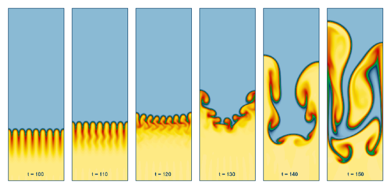
Figure 14: Symmetry breaking due to numerical noise and resulting instability. The snapshots are taken at times $ts_{\circ}/\delta=100,110,120,130,140,150.$

The images shown in Fig. 14 illustrate the propagation of a flame with eight wavelengths (with $L=16$, $G=4$) within the computational box with reflecting boundary conditions. The chosen parameters place the system well inside the unstable regime, and, by the time $t\approx 30\,\delta/s_{\circ}$ the system forms the curved travelling wave solution with wavelength $L=16$. This solution is exactly the same as the curved solution obtained in the half-wavelength computational box, propagates with the same speed, and remains unchanged until time $t\approx 100\,\delta/s_{\circ}$. (We note that the “wall effect” seen in this figure reflects both the presence of the walls (and choice of boundary condition at the walls) and the choice of phase for the initial perturbation.)

The symmetry of the initial conditions requires zero horizontal velocity at $x=nl/2$, $n=0,1,2,...$; this symmetry constraint is clearly broken for $t\gtrsim 100\delta/s_{\circ}$, and the travelling wave solution becomes violently unstable. The cause of this symmetry breaking is apparently accumulated numerical errors (noise) in the calculation. The source of this noise is the iterative solution for the stream function, so the noise has the wavelength of the computational domain. Since perturbations with larger wavelengths move faster, the system will eventually pick the travelling wave configuration corresponding to the largest possible wavelength — in the example shown, the wavelength $L=256$ (twice the box size).

The instability shown in Fig. 14 is not related to metastable behavior near ${G_{\rm cr}}$ discussed in Berestycki02 — both wavelengths present in the system are unstable for $G=4$. Rather, this simulation is an illustration of the fact that the small wavelengths have faster initial growth rates, but saturate at lower speeds. As a result, the instability exhibits a strong inverse cascade. More careful modelling of the noise introduced to the system, as well as more realistic treatment of boundary conditions at the walls, will be necessary to learn about the instability dynamics in an infinitely large domain; in particular, we believe that periodic boundary conditions should be imposed at the walls in order to study this problem further. In such a system we would expect unbounded growth of instability size; in a natural system we would expect the upper bound to be set by extrinsic spatial scales of the physical system.

IV Summary and Discussion

In this paper, we have studied the fully nonlinear behavior of diffusive pre-mixed flames in a gravitationally stratified medium, subject to the Boussinesq approximation. Our aim was both to compare our results for a viscous system with analytical (and empirical) results in the extant literature, and to better understand the phenomenology of fully nonlinear flames subject to gravity.

The essence of our results is that the numerics by and large confirm the Markstein and Pelcé & Clavin models, and extend their results to finite viscosity. We have shown explicitly that there is an extended regime for flames with finite flame front thickness for which the scaling on the $LG$ product applies (as it is known to do in the thin flame front limit). We have also examined the details of the flame front structure, and are able to give physically-motivated explanations for the observed scalings, for example, of the flow length scale behind the flame front on Prandtl number.

We have also observed a potentially new instability, which arises when noise breaks the symmetry constraint of the initial front perturbation. Our study suggest that this instability differs significantly from finger merging behavior of the non-linear Rayleigh-Taylor instability, in which the finger merging process resembles a continuous period-doubling phenomenon (e.g. adjacent fingers at any given generation merge in pairs). In contrast, the instability we observe seems to involve seeding, and strong growth, of modes with wavelengths much larger than the wavelength of the dominant front disturbance. We are currently investigating this instability in greater detail.

Finally, it is of some interest to consider the implication of our results for astrophysical nuclear flames, as arise in the context of white dwarf explosion. Using the results of Timmes & Woosly Timmes92 , we find that we would be far into the thin flame limit, with a density jump at the flame front $\Delta\rho\sim 0.1\rho$; hence our Boussinesq results are rather marginal in their applicability. Nevertheless, one can ask what the expected flame speed up would be in this limit; using our results we find that $s/s_{\circ}\approx(1+0.0486\,LG)^{1/2}$, with $LG=(\Delta\rho/\rho)\,lg/s_{\circ}^{2}$. Using the length scale of the order of a fraction of white the dwarf radius, $l\approx 10^{3}km$, gravitational acceleration on the surface of the star, $g\approx 10^{3}km/s^{2}$, and the laminar flame speed given by Timmes92 , $s_{\circ}\approx 100\,km/s$, we obtain $LG\approx 10$, and consequently a speed up of $s/s_{\circ}\approx 1.2$. Smaller laminar flame speeds would lead to the flame velocities independent of the laminar flame speed, $s=0.23\,(lg\Delta\rho/\rho)^{1/2}\approx 100\,km/s$, which could be also derived using the rising bubble model Layzer55 . Evidently, the flame speedup in this limit is very modest. Whether compressibility has much effect on this conclusion remains to be established and is now under active investigation.

V Acknowledgements

This work was supported by the Department of Energy under Grant No.B341495 to the Center for Astrophysical Thermonuclear Flashes at the University of Chicago.

References

- (1) J. Whelan and I. Iben, Astrophys. J. 186(3), 1007-1014 (1973).
- (2) E. Livne, Astrophys. J. 406, L17 (1993).
- (3) A. M. Khokhlov, Astrophys. J. 449, 695 (1995).
- (4) J. C. Niemeyer and W. Hillebrandt, Astrophys. J. 452, 779 (1995).
- (5) M. Reinecke, W. Hillebrandt, and J. C. Niemeyer, Astron. Astrophys. 347(2), 724 (1999).
- (6) V. N. Gamezo, A. M. Khokhlov, and E.S. Oran, BAAS 200, 1401 (2002).
- (7) P. Constantin, A. Kiselev, A. Oberman, and L. Ryzhik, Arch. Rat. Mech. Anal. 154, 53 (2000).
- (8) F. K. Röpke, W. Hillebrandt, and J. C. Niemeyer, astro-ph/0204036 (2002).
- (9) B. Audoly, H. Berestycki, and Y. Pomeau, Y., C.R.Acad. Sci., Ser. IIB 328, 255 (2000).
- (10) H. Berestycki, S. Kamin, and G. Sivashinsky, Interfaces and Free Boundaries 3, 361 (2001).
- (11) A. N. Kolmogorov, I. G. Petrovskii and N. S. Piskunov, Bull. Moskov. Gos. Univ. Mat. Mekh. 1 (1937), 1-25 (see Pelce88 pp. 105-130 for an English translation).
- (12) R. S. Tuminaro, M. Heroux, S. A. Hutchinson, and J.N. Shadid, Official AZTEC User’s Guide: Version 2.1 (1999).
- (13) Y.-N. Young, H. Tufo, A. Dudey, R. Rosner, J. Fluid Mech. 447, 377 (2001).
- (14) S. Chandrasekhar, Hydrodynamic and Hydromagnetic stability, Clarendron Press, Oxford, (1961).
- (15) L. D. Landau, and E. M. Lifshitz,Fluid Mechanics, 2nd edition, Pergamon Press, Oxford, (1987).
- (16) A. Kiselev and L. Ryzhik, private communication.
- (17) V. V. Bychkov and M. A. Liberman, Physics Reports 325, 115 (2000).
- (18) D. Layzer, Astrophys. J. 122, 1 (1955).
- (19) N. Vladimirova, P. Constantin, A. Kiselev, O. Ruchayskiy, and L. Ryzhik, physics/0212057 (2002).
- (20) Dynamics of curved fronts, P. Pelcé, Ed., Academic Press, (1988).
- (21) Ya. B. Zeldovich, G. I. Barenblatt, V. B. Librovich, and G. M. Makhviladze, The Mathematical Theory of Combustion and Explosions (Consultants Bureau, New York, 1985).
- (22) G. Darries, Propagation d’un Front de Flamme, Conferences: La Technique Modern, Congres de Mechanique Applique, Paris (1938).
- (23) L. D. Landau, Zh. Eksp. Teor. Fiz. 14, 240 (1944).
- (24) G. H. Markstein, Nonsteady Flame Propagation, (Pergamon Press, Oxford, 1964).
- (25) P. Pelcé and P. Clavin, J. Fluid Mech. 124, 219 (1982).
- (26) F. X. Timmes and S. E. Woosly, Astrophys. J. 396, 649 (1992).