Sub-picosecond compression by velocity bunching in a photo-injector

Abstract

We present an experimental evidence of a bunch compression scheme that uses a traveling wave accelerating structure as a compressor. The bunch length issued from a laser-driven radio-frequency electron source was compressed by a factor $>$3 using an S-band traveling wave structure located immediately downstream from the electron source. Experimental data are found to be in good agreement with particle tracking simulations.

I Introduction

In the recent years there has been an increasing demand on ultrashort electron bunches to drive short-wavelength free-electron lasers and study novel accelerating techniques such as plasma-based accelerators yurkovPRL ; barov . Short bunches are commonly obtained by magnetic compression. In this latter scheme, the bunch is compressed using a series of dipoles arranged in a chicane configuration such to introduce an energy-dependent pathlength. Therefore an electron bunch having the proper time-energy correlation can be shortened in the chicane. However, problems inherent to magnetic compression such as momentum spread and transverse emittance dilution due to the bunch self-interaction via coherent synchrotron radiation derbenev has brought back the idea of bunching the beam with radio-frequency (rf) structures haimson .

It was recently proposed to incorporate the latter method (henceforth named velocity bunching) into the next photo-injector designs serafini . The velocity bunching relies on the phase slippage between the electrons and the rf-wave that occurs during the acceleration of non ultra-relativistic electrons. In this paper after presenting a brief analysis of the velocity bunching scheme, we report on its exploration at the deep ultraviolet free-electron laser (DUV-FEL) facility of Brookhaven National Laboratory (BNL). The measurements are compared with numerical simulations performed with the computer program ASTRA astra .

II Analysis of the velocity bunching technique

In this section we elaborate a simple model that describes how the velocity bunching works. A more detailed discussion is given in Reference serafini .
An electron in an rf traveling wave accelerating structure experiences the longitudinal electric field:

$$E_{z}(z,t)=E_{o}\sin(\omega t-kz+\psi_{o})\mbox{,}$$ (1)

where $E_{o}$ is the peak field, $k$ the rf wavenumber and $\psi_{o}$ the injection phase of the electron with respect to the rf wave. Let $\psi(z,t)=\omega t-kz+\psi_{o}$ be the relative phase of the electron w.r.t the wave. The evolution of $\psi(t,z)$ can be expressed as a function of $z$ solely:

$$\frac{d\psi}{dz}=\omega\frac{dt}{dz}-k=\frac{\omega}{\beta c}-k=k\left(\frac{\gamma}{\sqrt{\gamma^{2}-1}}-1\right)\mbox{.}$$ (2)

Introducing the parameter $\alpha\doteq\frac{eE_{o}}{kmc^{2}}$, we write for the energy gradient kim :

$$\frac{d\gamma}{dz}=\alpha k\sin(\psi)\mbox{.}$$ (3)

The system of coupled differential equations (2) and (3) with the initial conditions $\gamma(z=0)=\gamma_{o}$ and $\psi(z=0)=\psi_{o}$ describe the longitudinal motion of an electron in the rf structure. Such a system is solved using the variable separation technique to yield:

$$\alpha\cos\psi+\gamma-\sqrt{\gamma^{2}-1}={\cal C}\mbox{.}$$ (4)

Or, expliciting $\psi$ as a function of $\gamma$:

$$\psi(\gamma)=\arccos\left(\frac{{\cal C}-\gamma+\sqrt{\gamma^{2}-1}}{\alpha}\right)\mbox{.}$$ (5)

Here the constant of integration is set by the initial conditions of the problem: ${\cal C}=\alpha\cos\psi_{o}+\gamma_{o}-\sqrt{\gamma_{o}^{2}-1}$. The latter equation gives insights on the underlying mechanism that provides compression. In order to get a simpler model, we consider the limit: $\psi_{\infty}\doteq\lim_{\gamma\rightarrow\infty}\psi(\gamma)=\mbox{arccos}\left(\cos(\psi_{o})+\frac{1}{2\alpha\gamma_{o}}\right)$; we have assumed $\gamma_{o}$ is larger than unit and did the approximation $\gamma_{o}-\sqrt{\gamma_{o}^{2}-1}\simeq 1/(2\gamma_{o})$. After differentiation of Eq. 5, given an initial phase $d\psi_{o}$ and energy $d\gamma_{o}$ extents we have for the final phase extent:

$$d\psi_{\infty}=\frac{\sin(\psi_{o})}{\sin(\psi_{\infty})}d\psi_{o}+\frac{1}{2\alpha\gamma_{o}^{2}\sin(\psi_{\infty})}d\gamma_{o}\mbox{.}$$ (6)

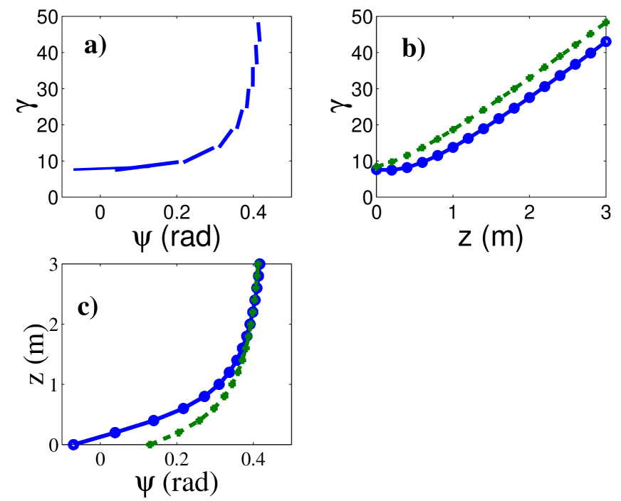
Figure 1: Simulation, using a two macro-particles model, of the velocity compression in a 3 m long traveling wave structure. The initial conditions are $(\psi_{o},\gamma_{o})$=(0,8) and the macro-particle spacing is $(\Delta\psi_{o},\Delta\gamma_{o})$=(0.1, 0.4). Plot a) shows snapshots at different $z$ of the longitudinal phase space each segment extremities is determined by the two macro-particles positions. Plots b) and c) present the energy gain and phase evolution of the two macro-particles versus $z$. In these two latter plots, solid lines represent the leading particle and dashed lines the trailing one.

Hence depending upon the incoming energy and phase extents, the phase of injection in the rf structure $\psi_{o}$ can be tuned to minimize the phase extent after extraction i.e. to ideally (under single-particle dynamics) make $d\psi_{\infty}\rightarrow 0$. We note that there are two contributions to $d\psi_{\infty}$: the first term $\partial\psi_{\infty}/\partial\psi_{o}$ comes from the phase slippage (the injection and extraction phases are generally different). The second term $\partial\psi_{\infty}/\partial\gamma_{o}$ is the contribution coming from the initial energy spread. To illustrate the compression mechanism we consider a two macro-particles model. In Figure 1 we present results obtained by numerically integrating the equation of motion for two non-interacting macro-particles injected into a 3 m long traveling wave structure. Given the incoming phase $\Delta\psi_{o}$ and energy $\Delta\gamma_{o}$ spreads between the two macro-particles, and the accelerating gradient of the structure (taken to be 20 MV/m), we can optimize the injection phase to minimize the bunch length at the structure exit.

III Experimental results

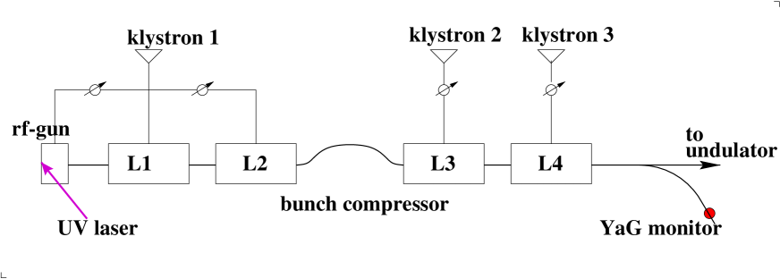
Figure 2: Overview of the Deep ultra-violet free-electron laser (DUV-FEL) accelerator. L1, L2, L3, and L4 are the four linac sections.

The measurement was carried out at the DUV-FEL facility of Brookhaven national laboratory duvfel . A block diagram of the linear accelerator is given in Fig. 2. The electron bunches of $\sim$4 MeV, generated by a laser-driven rf electron source, are accelerated by a series of four linac sections. The linac sections consist of 2.856 GHz traveling wave structures operating on the $2\pi/3$ accelerating mode. The structures are approximately 3 m long and can operate with an average accelerating voltage up to 20 MV/m. Nominally the bunch is shortened using a magnetic bunch compressor chicane located between the second and third linac sections. In this latter case, the linac sections L1, L3, L4 are ran on-crest while the linac L2 is operated to impart the proper time-energy correlation along the bunch to enable compression as the beam pass through the magnetic chicane.

To investigate the velocity bunching scheme, the linac section L1 was used as a buncher: its phase was varied and, for each phase setting, the section L2 was properly phased to maximize the beam energy with sections L3 and L4 turned off. The magnetic bunch compressor was turned off during the measurement. The nominal settings for the different rf and photo-cathode drive-laser parameters are gathered in Table 1.

parameter	value	units
laser injection phase	40 $\pm$ 5	rf-deg
laser radius on cathode	0.75 $\pm$ 0.1	mm
laser rms length	1.15 $\pm$ 0.1	ps
E-peak on cathode	83 $\pm$ 1	MV/m
L1 average accelerating field	10.5 $\pm$ 0.1	MV/m
L2 average accelerating field	13.2 $\pm$ 0.1	MV/m

Table 1: Nominal settings for the rf-gun, accelerating sections, and the photo-cathode drive-laser. The values have been directly measured or inferred from the beam properties.

The measurements of bunch length that follow are compared with simulations performed with the program ASTRA astra . ASTRA is a macro-particle tracking code based on a rotational symmetric space charge algorithm. It incorporates a detailed model for the traveling wave accelerating structure loew ; massimo . To perform the simulations we used the parameters values of Table 1. The laser transverse distribution was modeled by a radially uniform transverse distribution with 0.75 mm radius, and the time profile, measured using a single shot cross-correlation technique, was directly loaded into the simulations.

Both time- and frequency-domain techniques were used to characterize the bunching process as the phase of the linac L1 was varied.

The time-domain charge density was directly measured using the so-called zero-phasing method wang ; graveszp . In the present case, we use the linac section L3 to cancel the incoming time-energy correlation, and operate the linac L4 at zero-crossing to introduce a linear time-dependent energy chirp along the bunch (we have investigated both zero-crossing points). The bunch is then directed to a beam viewer (“YaG monitor” in Fig. 2) downstream from a $72^{\circ}$ angle spectrometer. The viewer, located at a dispersion (horizontal) of $\eta=907$ mm, allows the measurement of the bunch energy distribution. Unlike in Reference wang , the longitudinal phase space of beams issued from an rf electron source is not perfectly linear: because of the longitudinal space charge forces, the phase space generally has a third order distortion dowell . To analyze the impact of such a distortion on our bunch length measurement method, it is interesting to consider the Gaussian normalized longitudinal phase space $(s,\delta)$ density:

$${\cal P}(s,\delta)=\frac{1}{2\pi\sigma_{\delta}\sigma_{s}}\times\exp\left(-\frac{(\delta-h_{1}s-h_{3}s^{3})^{2}}{2\sigma_{\delta}^{2}}\right)\times\exp\left(-\frac{s^{2}}{2\sigma_{s}^{2}}\right)\mbox{.}$$ (7)

Here $\sigma_{s}$ and $\sigma_{\delta}$ are the bunch rms length and rms uncorrelated fractional momentum spread and $h_{1}$, $h_{3}$ are constants that quantify the linear and third order correlations of the longitudinal phase space. The zero-phasing measurement can then be analyzed in term of a sequence of numerical calculation based on Eq. 7: by computing and comparing the time and fractional momentum spread projections associated to ${\cal P}(s,\delta+C_{o}\times s)$. The constant $C_{o}$ depends on the incoming beam energy $E_{o}$, the accelerating voltage of the zero-phased linac section, the rf wavenumber $k_{rf}$, and dispersion wang : $C_{o}=\pm\frac{E_{o}}{\eta V_{rf}k_{rf}}$ the $\pm$ sign reflects the two possible zero-crossing points.

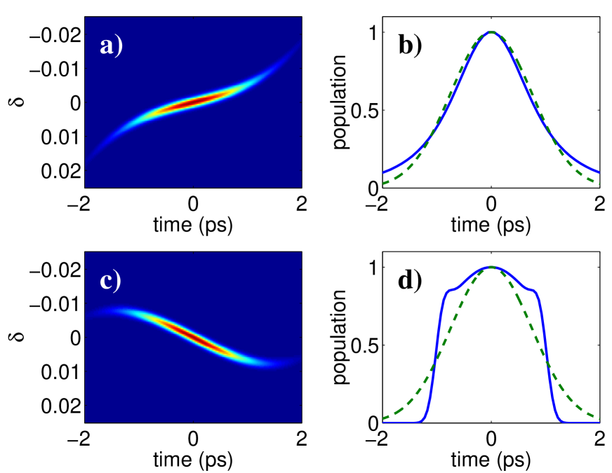
Figure 3: Simulation of the zero-phasing method for a distorted incoming longitudinal phase space. The images a) and c) depict the phase spaces after the bunch as passed the zero-phasing traveling wave structure for the ”positive” (upper plots) and ”negative” (lower plots) zero-crossing points. The plots b) and d) are the corresponding projections. In these plots we compare the time projection (dashed lines) with the one deduced from the fractional momentum spread projection (solid lines). The time $>0$ corresponds to the bunch tail.

An example of such a calculation is presented in Fig. 3. To generate the presented data we started with a longitudinal phase space which has a third order distortion but no linear correlation (as it should be downstream from linac L3) we then set the constant $C_{o}$ to have a full-width fractional momentum spread of approximately $1.5$ % similar to the value imposed by the finite size of the viewer (diameter $\sim$15 mm) used for the measurement of the bunch energy distribution. The Figure 3 demonstrates the impact of the third order distortion in the longitudinal phase space: depending on the chosen zero-crossing phase, it contributes to an elongation or a contraction of the measured time profile compared to the real profile. For the rms bunch length measurements reported hereafter we computed the average bunch length measured for the two zero-crossing points and reported the difference as an error bar. For the reported bunch profiles we use the bunch profile corresponding to the case when the phase space has no fold over. Hence we expect the bunch time-profile reported hereafter to be longer than in reality.

As the phase of the linac section L1 was varied and L2 tuned to maximize the energy gain, the beam energy was measured. The so-obtained energy variation versus the phase of the linac L1 is compared with the simulations for the nominal operating point (see Table 1) in Fig. 4 and the corresponding plot for the bunch length is shown in Fig. 5. As predicted, we observed that operating the linac at lower phases (thereby giving the bunch head less energy than the tail) provides some compression. The parametric dependence of the rms bunch length on the phase of linac L1 is found to be in good agreement with the simulation predictions. Two cases of measured and simulated bunch time-profile are presented in Fig. 6. Again, the agreement between simulation and experiment is fairly good taking into account the uncertainties associated to the zero-phasing method. Noteworthy is the achieved peak current of $\sim$150 A.

The frequency-domain technique is based on the measurement of the coherent radiation emitted by the electron bunch via some electromagnetic process. In the coherent regime (i.e. for frequencies $\omega\sim 2\pi/\sigma_{t}$ where $\sigma_{t}$ is the rms bunch duration) the radiated power scales with the squared charge and depends on the bunch form factor. Thus it provides indirect informations on the bunch time-profile. In DUV-FEL, we detect the far-field radiation associated to the geometric wake field caused by aperture variation along the accelerator (e.g. the irises of the rf-structure). The radiation shining out of a single-crystal quartz vacuum window, located prior to the linac section L3, was detected with a He-cooled bolometer. The detection system, composed of the bolometer and the vacuum extraction port, can transmit radiation within the frequency range $[\omega_{l},\omega_{u}]\simeq[1.2,50]$ THz. The lower and upper frequency limits being respectively due to diffraction effects related to the finite size of the detector and transmission function of the vacuum extraction port. Given the bunch charge $Q$ and the Fourier transform of the bunch time-profile $\tilde{S}(\omega)$, the power is expected to scale as $P\sim Q^{2}\int_{\omega_{l}}^{\omega_{u}}d\omega|\tilde{S}(\omega)|^{2}\propto Q^{2}/\sigma_{t}$ (see annex for details). The typical signal observed as the charge is varied is presented in Fig. 7: the observed nonlinear behavior confirms that the emitted radiation is not incoherent. From simulation we expect the power to scale as $P\propto Q^{1.37}$ (see annex for details) a number close to the one resulting from the fit of the data: $P\propto Q^{1.57}$.

In Figure 8, the measured bolometer output signal versus the phase of L1 is compared with the expectation (1) calculated from the simulated phase space density and (2) computed from the measured bunch time profile obtained by zero-phasing. As expected the increase of the coherent signal is an unambiguous signature of the bunch being compressed (the charge was monitored during the measurement and remained constant to 200$\pm$20 pC).
The data points computed from the measured time profile $f_{meas}$ were obtained by numerically computing the Fourier transform of the bunch time-profile (using a FFT algorithm) and by performing the integration:

$$f_{meas}=\int_{\omega_{l}}^{\omega_{u}}d\omega|\tilde{S}(\omega)\times R(\omega)|^{2}\mbox{.}$$ (8)

where $R(\omega)$ stands for the frequency response of the detection system.

To generate the data points from the simulated phase space distributions $f_{simu}$ we write the time-profile, $S(t)$ as a Klimontovitch distribution:

$$S(t)=\frac{1}{N}\sum_{i=1}^{N}\delta(t_{i}-t)\mbox{,}$$ (9)

$N$ being the number of macro-particle used (50000 in the simulations presented hereafter) and $t_{i}$ the time of arrival of the $i$-th macro-particle. Eq. (9) allows to write the integrated power as:

$$f_{simu}=\frac{1}{N^{2}}\int_{\omega_{l}}^{\omega_{u}}d\omega|R(\omega)|^{2}\left(\left[\sum_{i=1}^{N}\cos(\omega t_{i})\right]^{2}+\left[\sum_{i=1}^{N}\sin(\omega t_{i})\right]^{2}\right)\mbox{.}$$ (10)

Though Figure 8 shows the signal increases as the bunch is compressed, there are discrepancies between the measurement and the two calculations for the short bunch case, we believe this is due to the lack of a precise knowledge of the transmission line frequency response.

IV Conclusion

We have measured the bunch length dependence on the phase of a traveling wave accelerating structure located just downstream from an rf electron source. We could compress the bunch by a factor ¿3, down to $\sim$0.5 ps, for a bunch charge of 200 pC. In our experimental setup, a stronger compression is currently difficult to achieve without significantly impinging the transverse phases-pace quality. The linac section used for the compression also plays a crucial role in achieving low emittance since it quickly accelerates the beam at energies of approximately 60 MeV thereby freezing the transverse phase space. Hence operating the first linac far off-crest reduces the final energy and impact the emittance since transverse space charge forces scale as $1/\gamma^{2}$. An improvement of our experiment would be to surround the accelerating structure used as a bunch compressor with a solenoidal lens to enable a better control of the beam transverse envelope and emittance bacci ; boscolo .

V Acknowledgments

This work was sponsored by US-DOE grant number DE-AC02-76CH00016 and by the Deutsches Elektronen-Synchrotron institute. We are indebted to Luca Serafini of Univ. Milano for carefully reading and commenting the manuscript.

Appendix: Dependence of radiated power on bunch charge

Let’s consider the case of a Gaussian distribution:

$$S(t)=\frac{1}{\sqrt{2\pi\sigma_{t}^{2}}}\exp\left(\frac{-t^{2}}{2\sigma_{t}^{2}}\right).$$

The corresponding bunch form factor takes the form:

$$|S(\omega)|^{2}=|\int_{-\infty}^{+\infty}S(t)\exp{-i\omega t}|^{2}=\exp\left(-\sigma^{2}_{t}\omega^{2}\right),$$

and the integrated bunch form factor in the $[\omega_{l},\omega_{u}]$ frequency interval is:

$$f=\int_{\omega_{l}}^{\omega_{u}}d\omega\exp\left(-\sigma_{t}^{2}\omega^{2}\right).$$

The integration of the latter equation can be written in term of “error” function:

$$f=\frac{\sqrt{\pi}}{2\sigma_{t}}\left(\mbox{erf}(\sigma_{t}\omega_{u})-\mbox{erf}(\sigma_{t}\omega_{l})\right).$$ (11)

Taking into account the limit of the erf function,

$$\lim_{z\rightarrow\infty}\mbox{erf}(z)=1\mbox{, and}$$ (12)

$$\lim_{z\rightarrow 0}\mbox{erf}(z)=0\mbox{,}$$

and assuming the frequency range is so that $\sigma_{t}\omega_{u}\gg 1$ and $\sigma_{t}\omega_{l}\ll 1$, we finally have for the radiated power:

$$P\propto Q^{2}\times f\propto\frac{Q^{2}}{\sigma_{t}}\mbox{.}$$ (13)

Figure 9 shows the dependence of the bunch length versus the charge expected from simulations . We find $\sigma_{t}\propto Q^{0.43}$ and thus we would expect the radiated power to be $P\propto Q^{1.57}$ which is close to the value deduced from the fit of the measurement presented in Fig. 7: $P\propto Q^{1.37}$.

Figure 4: Total energy versus phase of linac section L1. The points are measurements obtained parasitically to the bunch length measurement. The solid line is a simulation result.

Figure 5: Rms bunch length versus phase of the linac section L1.

Figure 6: Comparison of the bunch time-profile for L1 on crest ($\phi_{L1}=0^{\circ}$), and $-82^{\circ}$ off-crest. Plot a) was generated by tracking simulation; plot b) is a direct measurement using the zero-phasing method. The time $>0$ corresponds to the bunch tail

Figure 7: Dependence of bolometer signal versus bunch charge. The circles are measurement, the line is a fit of the measurement using a $\alpha\times Q^{\beta}$ law, the result gives $\beta=1.37\pm 0.06$.

Figure 8: Integrated bunch form factor $f$ normalized to its value at $\phi_{L1}=38^{\circ}$. $f_{bolom}$, $f_{meas}$, and $f_{simu}$ correspond respectively to measurement with the bolometer, computation from the measured time-profiles and computation from the simulation-generated time profiles.

Figure 9: Simulated dependence of bunch length versus charge. The circles are simulation results, the line is a fit to the simulation using a $\alpha\times Q^{\beta}$ law, the result gives $\beta=0.437\pm 0.007$.

References

- (1) Ayvazian V., et al, Eur. Jour. Phys. D 20:149-155 (2002)
- (2) Barov N., et al, Phys. Rev. ST-AB(3):011301 (2000)
- (3) Kim, K.-J., Nucl. Instr. Meth. A 275:201-218 (1989)
- (4) Derbenev Ya., et al., TESLA-FEL report No. 95-05, DESY Hamburg (1995)
- (5) Haimson H., Nucl. Instr. Meth. 39:13-34 (1966)
- (6) Serafini L., Ferrario M., “Velocity bunching in photo-injectors”, in Physics of, and science with, the X-ray free-electron laser edited by S. Chattopadyay et al. AIP conference proceedings 581, 87-106 (2001)
- (7) Flöttmann K. Astra user manual DESY (2000). The program and its documentation are available from the web-site: http://www.desy.de/~mpyflo
- (8) Loew G.A., Miller R.H., Early R.A, Bane K.L. “Computer calculation of traveling-wave periodic structure properties”, SLAC-PUB-2296 Stanford (1979)
- (9) Ferrario M., Clendemin J.E., Palmer D.T., Rosenzweig J.B., Serafini L., “HOMDYN study for the LCLS rf photo-injector”, SLAC-PUB-9400 Stanford (2000) and report LNF-00/004 INFN-Frascati (2000)
- (10) Dowell D., Joly S., Loulergue A., in Proceeding of PAC 1997 Vancouver, 2684-2686 (1998)
- (11) Yu, L.-H. et al, in Proceeding of PAC 2001 Chicago, 2830-2832 (2002)
- (12) Wang D.X., Krafft G.A., and Sinclair C.K. Phys. Rev. E57(2):2283-2286 (1998)
- (13) Graves, W. et al, in Proceeding of PAC 2001 Chicago, 2224-2226 (2002)
- (14) Serfini L., Bacci A., and Ferrario M., in Proceeding of PAC 2001 Chicago, 2242-2244 (2002)
- (15) Boscolo M. et al, in Proceeding of EPAC 2002 Paris, 1762-1764 (2002)