Binary $N$-Step Markov Chain as an Exactly Solvable Model of Long-Range Correlated Systems

Abstract

A theory of systems with long-range correlations based on the consideration of binary N-step Markov chains is developed. In our model, the conditional probability that the $i$-th symbol in the chain equals zero (or unity) is a linear function of the number of unities among the preceding $N$ symbols. The model allows exact analytical treatment. The correlation and distribution functions as well as the variance of number of symbols in the words of arbitrary length $L$ are obtained analytically and numerically. A self-similarity of the studied stochastic process is revealed and the similarity transformation of the chain parameters is presented. The diffusion equation governing the distribution function of the $L$-words is explored. If the persistent correlations are not extremely strong, the distribution function is shown to be the Gaussian with the variance being nonlinearly dependent on $L$. The applicability of the developed theory to the coarse-grained written and DNA texts is discussed.

I Introduction

The problem of long-range correlations is one of the topics of current research in the statistical mechanics. The stochastic processes with strong correlations have been observed in numerous systems. Examples include the natural languages, the DNA sequences, etc. stan ; prov .

One of the efficient methods to investigate the correlated systems is based on a decomposition of the space of states into a finite number of parts labelled by definite symbols. This procedure referred to as coarse graining is accompanied by the loss of short-range memory between symbols but does not affect and does not damage the robust invariant statistical properties of the long-range correlated sequences. In terms of the power spectrum, one loses only the short-wave part of the spectrum. The most frequently used method of the decomposition is based on the introduction of two parts of the phase space. In other words, it consists in mapping the two parts of states onto two symbols, say 0 and 1. Thus, the problem is reduced to the investigation into the statistical properties of the binary sequences. This method is applicable for the examination of the both discrete and continuous systems.

One of the ways to get a correct insight into the nature of correlations in a system consists in an ability of constructing a mathematical object (for example, a correlated sequence of symbols) possessing the same statistical properties as the initial system. There are many algorithms to generate long-range correlated sequences: the inverse Fourier transform czir , the expansion-modification Li method li , the Voss procedure of consequent random addition voss , the correlated Levy walks shl , etc. czir . We believe that from among the above-mentioned methods, using the Markov chains is one of the most important. We would like to demonstrate this statement in the present paper.

In the next sections, the statistical properties of the binary many-steps Markov chain is examined. In spite of the long-time history of studying the Markov sequences (see, for example, nag ; kant ; trib ), the concrete expressions for the variance of sums of random variables in such strings have not been obtained yet. Our model operates with two parameters governing the conditional probability of the discrete Markov process, specifically with the memory length $N$ and the correlation parameter $\mu$. The correlation and distribution functions as well as the variance $D$ being nonlinearly dependent on the length $L$ of a word are derived analytically and calculated numerically. The nonlinearity of the $D(L)$ function reflects the strong correlations in the system. The evolved theory is applied to the coarse-grained written texts and dictionaries, and to DNA strings as well.

II Formulation of the problem

II.1 Markov Processes

Let us consider a stationary binary sequence of symbols, $a_{i}=\{0,1\}$. To determine the $N$-step Markov chain we have to introduce the conditional probability $P(a_{i}=0\mid a_{i-N},a_{i-N+1},\dots,a_{i-1})$ of following the definite symbol (for example, zero) after symbols $a_{i-N},a_{i-N+1},\dots,a_{i-1}$. Thus, it is necessary to define $2^{N}$ values of the $P$-function corresponding to each possible configuration of the symbols $a_{i-N},a_{i-N+1},\dots,a_{i-1}$. We suppose that the $P$-function has the form,

$$P(a_{i}=0\mid a_{i-N},a_{i-N+1},\dots,a_{i-1})=\frac{1}{N}\sum\limits_{k=1}^{N}f(a_{i-k},k).$$ (1)

It is reasonable to assume the function $f$ to be decreasing with an increase of the distance $k$ between the symbols $a_{i-k}$ and $a_{i}$ in the Markov chain. However, for the sake of simplicity we consider here a step-like memory function $f(a_{i-k},k)$ independent of the second argument $k$. As a result, our model is characterized by three parameters only, specifically by $f(0)$, $f(1)$, and $N$:

$$P(a_{i}=0\mid a_{i-N},a_{i-N+1},\dots,a_{i-1})=\frac{1}{N}\sum\limits_{k=1}^{N}f(a_{i-k}).$$ (2)

Note that the probability $P$ in Eq. (2) depends on the numbers of symbols 0 and 1 in the $N$-word but is independent of the arrangement of the elements $a_{i-k}$. We also suppose that

$$f(0)+f(1)=1.$$ (3)

This relation provides the statistical equality of the numbers of symbols zero and unity in the Markov chain under consideration. In other words, the chain is non-biased. Indeed, taking into account Eqs. (2) and (3) and the sequence of equations,

$$P(a_{i}=1|a_{i-N},\dots,a_{i-1})=1-P(a_{i}=0|a_{i-N},\dots,a_{i-1})=\frac{1}{N}\sum\limits_{k=1}^{N}f(\tilde{a}_{i-N})=P(a_{i}=0\mid\tilde{a}_{i-N},\dots,\tilde{a}_{i-1}),$$ (4)

one can see the symmetry with respect to interchange $\tilde{a}_{i}\leftrightarrow a_{i}$ in the Markov chain. Here $\tilde{a}_{i}$ is the symbol opposite to $a_{i}$, $\tilde{a}_{i}=1-a_{i}$. Therefore, the probabilities of occurring the words $(a_{1},\dots,a_{L})$ and $(\tilde{a}_{1},\dots,\tilde{a}_{L})$ are equal to each other for any word length $L$. At $L=1$ this yields equal average probabilities of occurring $0$ and $1$ in the chain.

Taking into account the symmetry of a conditional probability $P$ with respect to a permutation of symbols $a_{i}$ (see Eq. (2)), we can simplify the notations and introduce the conditional probability $p_{k}$ of occurring the symbol zero after the $N$-word containing $k$ unities, e.g., after the word $\underbrace{(11...1}_{k}\;\underbrace{00...0}_{N-k})$,

$$p_{k}=P(a_{N+1}=0\mid\underbrace{11\dots 1}_{k}\;\underbrace{00\dots 0}_{N-k})=\frac{1}{2}+\mu(1-\frac{2k}{N}),$$ (5)

with the correlation parameter $\mu$ being defined by the relation

$$\mu=f(0)-\frac{1}{2}.$$ (6)

We focus our attention on the region of $\mu$ determined by the persistence inequality $0\leq\mu<1/2$. Nevertheless, the major part of our results is valid for the anti-persistent region $-1/2<\mu<0$ as well.

A similar rule for the production of an $N$-word $(a_{1},\dots,a_{N})$ following after a word $(a_{0},a_{1},\dots,a_{N-1})$ was suggested in Ref. kant . However, the conditional probability $p_{k}$ of occurring the symbols $a_{N}$ does not depend on the previous ones in the model kant .

II.2 Statistical characteristics of the chain

In order to investigate the statistical properties of the Markov chain, we consider the distribution $W_{L}(k)$ of the words of definite length $L$ by the number $k$ of unities in them,

$$k_{i}(L)=\sum\limits_{l=1}^{L}a_{i+l},$$ (7)

and the variance of $k$,

$$D(L)=\overline{k^{2}}-\overline{k}^{2},$$ (8)

where

$$\overline{f(k)}=\sum\limits_{k=0}^{L}f(k)W_{L}(k).$$ (9)

If $\mu=0,$ one arrives at the known result for the non-correlated Brownian diffusion,

$$D(L)=L/4.$$ (10)

We will show that the distribution function $W_{L}(k)$ for the sequence determined by Eq. (5) (with nonzero but not extremely close to 1/2 parameter $\mu$) is the Gaussian with the variance $D(L)$ nonlinearly dependent on $L$.

II.3 Main equation

For the stationary Markov chain, the probability $b(a_{1}a_{2}\dots a_{N})$ of occurring a certain word $(a_{1},a_{2},\dots,a_{N})$ satisfies the equation,

$$b(a_{1}\dots a_{N})=\sum_{a=0,1}b(aa_{1}\dots a_{N-1})P(a_{N}\mid a,a_{1},\dots,a_{N-1}).$$ (11)

Thus, we have $2^{N}$ homogeneous algebraic equations for $2^{N}$ words and the normalization equation $\sum b=1$. The set of equations can be essentially simplified owing to the following statement.

Proposition $\spadesuit$: The probability $b(a_{1}a_{2}\dots a_{N})$ depends on the number $k$ of unities in the $N$-word only but is independent of the arrangement of symbols in the word $(a_{1},a_{2},\dots,a_{N})$.

This statement illustrated by Fig. 1 is valid owing to the chosen simple model (2), (5) of the Markov chain. It can be easily verified directly by the substitution of the obtained below solution Eq. (13) into set (11). Proposition $\spadesuit$ leads to the very important property of isotropy: any word $(a_{1},a_{2},\dots,a_{L})$ appears with the same probability as the inverted one, $(a_{L},a_{L-1},\dots,a_{1})$.

Figure 1: The probability of occurring a word $(a_{1},a_{2},\dots,a_{N})$ vs its number $z$ in the binary code, $z=\sum_{i=1}^{N}a_{i}\cdot 2^{i-1}$ for $N=8$, $\mu=0.4$.

Let us apply set of Eqs. (11) to the word $(\underbrace{11\dots 1}_{k}\;\underbrace{00\dots 0}_{N-k})$:

$$b(\underbrace{11\dots 1}_{k}\;\underbrace{00\dots 0}_{N-k})=b(0\underbrace{11\dots 1}_{k}\;\underbrace{00\dots 0}_{N-k-1})p_{k}+b(1\underbrace{11\dots 1}_{k}\;\underbrace{00\dots 0}_{N-k-1})p_{k+1}.$$ (12)

This yields the recursion relation for $b(k)=b(\underbrace{11...1}_{k}\;\underbrace{00...0}_{N-k})$,

$$b(k)=\frac{1-p_{k-1}}{p_{k}}b(k-1)=\frac{N-2\mu(N-2k-2)}{N+2\mu(N-2k)}b(k-1).$$ (13)

III Distribution function of $L$-words

In this section we investigate the statistical properties of the Markov chain, specifically, the distribution of the words of definite length $L$ by the number $k$ of unities in them. The length $L$ can also be interpreted as the number of jumps of some particle over an integer-valued 1-D lattice or as the time of the diffusion imposed by the Markov chain under consideration. The form of the distribution function $W_{L}(k)$ depends essentially on the relation between the word length $L$ and the memory length $N$. Therefore, we start our study with the simplest case, $L=N$.

III.1 Statistics of $N$-words

The value $b(k)$ is the probability that an $N$-word contains $k$ unities with a definite order of symbols $a_{i}$. Therefore, the probability $W_{N}(k)$ that an $N$-word contains $k$ unities with arbitrary order of symbols $a_{i}$ is $b(k)$ multiplied by the number $\mathrm{C}_{N}^{k}=N!/k!(N-k)!$ of different permutations of $k$ unities in the $N$-word,

$$W_{N}(k)=\text{C}_{N}^{k}b(k).$$ (14)

Combining Eqs. (13) and (14), we get

$$W_{N}(k)=W_{N}(0)\text{C}_{N}^{k}\frac{\Gamma(n+k)\Gamma(n+N-k)}{\Gamma(n)\Gamma(n+N)}$$ (15)

with the parameter $n$ defined by

$$n=\frac{N(1-2\mu)}{4\mu}.$$ (16)

The normalization constant $W_{N}(0)$ can be obtained from the equality,

$$\sum\limits_{k=0}^{N}\text{C}_{N}^{k}b(k)=1.$$ (17)

Note that the distribution $W_{N}(k)$ is an even function of the variable $\kappa=k-N/2$,

$$W_{N}(N-k)=W_{N}(k).$$ (18)

This fact is a direct consequence of the above-mentioned statistical equivalency of zeros and unities in the Markov chain under consideration. Let us analyze the distribution function $W_{N}(k)$ for different relations between the parameters $N$ and $\mu$.

III.1.1 Limiting case of weak persistence, $n\gg 1$

In the absence of correlations, $\mu\rightarrow 0$, Eq. (15) and the Stirling formula yield the Gaussian distribution at $k,\,N,\,N-k\gg 1$. In the most interesting case of not too strong persistence, $n\gg 1$, one can also obtain the Gaussian form for the distribution function,

$$W_{N}(k)=\frac{1}{\sqrt{2\pi D(N)}}\exp\left\{-\frac{(k-N/2)^{2}}{2D(N)}\right\},$$ (19)

with the $\mu$-dependent variance,

$$D(N)=\frac{N}{4(1-2\mu)}.$$ (20)

Equation (19) says that the $N$-words with equal numbers of zeros and unities, $k=N/2$, are mostly probable. Note that the persistence results in an increase of the variance $D(N)$ with respect to its value $N/4$ at $\mu=0$. In other words, the persistence is conductive to the intensification of the diffusion. Inequality $n\gg 1$ provides $D(N)\ll N^{2}$. Therefore, despite the increase of $D(N)$, the fluctuations of $(k-N/2)$ of the order of $N$ are exponentially small.

III.1.2 Intermediate case, $n\sim 1$

If the parameter $n$ is an integer of the order of unity, the distribution function $W_{N}(k)$ is a polynomial of degree $2(n-1)$. In particular, at $n=1$, the function $W_{N}(k)$ is constant,

$$W_{N}(k)=\frac{1}{N+1}.$$ (21)

At $n\neq 1,$ $W_{N}(k)$ has a maximum at the middle of the interval $[0,N]$.

III.1.3 Limiting case of strong persistence, $n\ll 1$

In this situation, $W_{N}(k)$ assumes the maximal values at $k=0$ and $k=N$,

$$W_{N}(1)=W_{N}(0)\frac{nN}{N-1}\ll W_{N}(0).$$ (22)

Formula (22) describes the sharply decreasing $W_{N}(k)$ as $k$ changes from $0$ to $1$ (and from $N$ to $N-1$). Then, at $1<k<N/2$, the function $W_{N}(k)$ decreases more slowly with an increase in $k$,

$$W_{N}(k)=W_{N}(0)\frac{nN}{k(N-k)}.$$ (23)

At $k=N/2,$ the probability $W_{N}(k)$ achieves its minimal value,

$$W_{N}\left(\frac{N}{2}\right)=W_{N}(0)\frac{4n}{N}.$$ (24)

The values $W_{N}(0)=W_{N}(N)$ are nearly $1/2$ to a logarithmic accuracy.

The evolution of the distribution function $W_{N}(k)$ from the Gaussian form to the inverse one with a decrease of the parameter $n$ is shown in Fig. 2. Below we restrict ourselves to the case of weak persistence, $n\gg 1$.

Formulas (19) and (20) describe the statistical properties of $L$-words for the fixed ”diffusion time” $L=N$. It is necessary to look into the distribution function $W_{L}(k)$ for the general situation, $L\neq N$. We start the analysis with $L<N$.

Figure 2: The distribution function $W_{N}(k)$ for $N$=20 and different values of the parameter $n$ shown near the curves.

III.2 Statistics of $L$-words with $L<N$

III.2.1 Distribution function $W_{L}(k)$

The distribution function $W_{L}(k)$ at $L<N$ can be given as

$$W_{L}(k)=\sum\limits_{i=k}^{k+N-L}b(i)\text{C}_{L}^{k}\text{C}_{N-L}^{i-k}.$$ (25)

This equation follows from the consideration of $N$-words consisting of two parts,

$$(\underbrace{a_{1},\dots,a_{N-L},}_{i-k\text{ unities}}\;\underbrace{a_{N-L+1},\dots,a_{N}}_{k\text{ unities}}).$$ (26)

The total number of unities in this word is $i$. The right-hand part of the word ($L$-sub-word) contains $k$ unities. The remaining $i-k$ unities are situated within the left-hand part of the word ($(N-L)$-sub-word). The multiplier $\mathrm{C}_{L}^{k}\mathrm{C}_{N-L}^{i-k}$ in Eq. (25) takes into account all possible permutations of the symbols ”1” within the $N$-word on condition that the $L$-sub-word always contains $k$ unities. Then we perform the summation over all possible values of the number $i$. Note that Eq. (25) is valid due to the main proposition $\spadesuit$ formulated in Subsec. C of the previous section.

In this subsection, we focus our attention on the most important limiting case $n,\;k,\;L-k\gg 1$. The straightforward calculations with using the Stirling formula give the result,

$$W_{L}(k)=\frac{1}{\sqrt{2\pi D(L)}}\exp\left\{-\frac{(k-L/2)^{2}}{2D(L)}\right\}$$ (27)

with

$$D(L)=\frac{L}{4}(1+mL),\quad m=\frac{1}{2n}=\frac{2\mu}{N(1-2\mu)}.$$ (28)

The last equation allows one to analyze the behavior of the variance $D(L)$ with an increase in the “diffusion time” $L$. At small $mL\ll 1$ the dependence $D(L)$ follows the classical law of the Brownian diffusion, $D(L)\approx L/4$. Then, at $mL\sim 1$, the function $D(L)$ becomes super-linear and meets the value (20) at $L=N$.

Such an unusual behavior of the variance $D(L)$ raises an issue as to what particular type of the diffusion equation corresponds to the nonlinear dependence $D(L)$ in Eq. (28). In the following subsection, when solving this problem, we will obtain the conditional probability $p^{(0)}$ of occurring the symbol zero after a given $L$-word with $L<N$. The ability to find $p^{(0)}$, with some reduced information about preceding symbols being available, is very important for the study of the self-similarity of the Markov chain (see Subsubsec. 3 of this Subsection).

III.2.2 Generalized diffusion equation

It is quite obvious that the distribution $W_{L}(k)$ satisfies the equation

$$W_{L+1}(k)=W_{L}(k)p^{(0)}(k)+W_{L}(k-1)p^{(1)}(k-1).$$ (29)

Here $p^{(0)}$ is the probability of occurring ”0” after an average-statistical $L$-word containing $k$ unities and $p^{(1)}$ is the probability of occurring ”1” after an $L$-word containing $k-1$ unities. At $L<N$, the probability $p^{(0)}$ can be written as

$$p^{(0)}=\frac{1}{W_{L}(k)}\sum\limits_{i=k}^{k+N-L}p_{i}b(i)\mathrm{C}_{L}^{k}\mathrm{C}_{N-L}^{i-k}.$$ (30)

The product $b(i)\mathrm{C}_{L}^{k}\mathrm{C}_{N-L}^{i-k}$ in this formula represents the conditional probability of occurring the $N$-word containing $i$ unities, the right-hand part of which, the $L$-sub-word, contains $k$ unities (compare with Eqs. (25), (26)).

The product $b(i)\mathrm{C}_{N-L}^{i-k}$ in Eq. (30) is a sharp function of $i$ with a maximum at some point $i=i_{0}$ whereas $p_{i}$ obeys linear law (5). This implies that $p_{i}$ can be factored out of the summation sign being taken at point $i=i_{0}$. The asymptotical calculation shows that point $i_{0}$ is described by the equation,

$$i_{0}=\frac{N}{2}-\frac{L/2}{1-2\mu(1-L/N)}\left(1-\frac{2k}{L}\right).$$ (31)

Expression (5) taken at point $k=i_{0}$ gives the desired formula for $p^{(0)}$ because

$$\sum\limits_{i=k}^{k+N-L}b(i)\mathrm{C}_{L}^{k}\mathrm{C}_{N-L}^{i-k}$$ (32)

is obviously equal to $W_{L}(k)$. Thus, we have

$$p^{(0)}(k)=\frac{1}{2}+\frac{\mu L}{N-2\mu(N-L)}\left(1-\frac{2k}{L}\right).$$ (33)

Let us consider a very important fact following from Eq. (31). If the concentration of unities in the right-hand part of the word (26) is higher than $1/2$, $k/L>1/2$, then the most probable concentration $(i_{0}-k)/(N-L)$ of unities in the left-hand part of this word is likewise increased, $(i_{0}-k)/(N-L)>1/2$. At the same time, the concentration $(i_{0}-k)/(N-L)$ is less than $k/L$,

$$\frac{1}{2}<\frac{i_{0}-k}{N-L}<\frac{k}{L}.$$ (34)

This means that the increased concentration of unities in the $L$-words is necessarily accompanied by the existence of a certain tail with an increased concentration of unities as well. We name such a phenomenon as the macro-persistence. An analysis performed in the next section will indicate that the correlation length $l_{c}$ of this tail is $\gamma N$ with $\gamma\geq 1$ dependent on the parameter $\mu$ only. It is evident from the above-mentioned property of the isotropy of the Markov chain that there are two correlation tails from the both sides of the $L$-word.

By going over to the continuous limit in Eq. (29) and using Eq. (33) and the relation $p^{(1)}(k-1)=1-p^{(0)}(k-1)$, we obtain the diffusion equation generalized to the case of the correlated Markov process,

$$\frac{\partial W}{\partial L}=\frac{1}{8}\frac{\partial^{2}W}{\partial\kappa^{2}}-\eta(L)\left(\kappa\frac{\partial W}{\partial\kappa}+W\right),$$ (35)

with $\kappa=k-L/2$ and

$$\eta(L)=\frac{2\mu}{(1-2\mu)N+2\mu L}.$$ (36)

Equation (35) has a solution of the Gaussian form Eq. (27) with the variance $D(L)$ satisfying the ordinary differential equation,

$$\frac{\mathrm{d}D}{\mathrm{d}L}=\frac{1}{4}+2\eta(L)D.$$ (37)

Its solution with the boundary condition $D(0)=0$ coincides with (28).

III.2.3 Self-similarity of the persistent Brownian diffusion

In this subsection we point out one of the most important properties of the Markov chain being considered, namely, its self-similarity. Let us reduce the $N$-step Markov sequence by regularly (or randomly) removing some symbols and introduce the decimation parameter $\lambda$,

$$\lambda=N^{\ast}/N\leq 1.$$ (38)

Here $N^{\ast}$ is a renormalized memory length for the reduced $N^{\ast}$-step Markov chain. According to Eq. (33), the conditional probability $p_{k}^{\ast}$ of occurring the symbol zero after $k$ unities among the preceding $N^{\ast}$ symbols is described by the formula,

$$p_{k}^{\ast}=\frac{1}{2}+\mu^{\ast}\left(1-\frac{2k}{N^{\ast}}\right),$$ (39)

with

$$\mu^{\ast}=\mu\frac{\lambda}{1-2\mu(1-\lambda)}.$$ (40)

The comparison of Eqs. (5) and (39) shows that the reduced chain possesses the same statistical properties as the initial one but is characterized by the renormalized parameters ($N^{\ast}$, $\mu^{\ast}$) instead of ($N$, $\mu$). Thus, Eqs. (38) and (40) determine the one-parametrical renormalization of the parameters of the stochastic process defined by Eq. (5).

The astonishing property of the reduced sequence consists in that the variance $D^{\ast}(L)$ is invariant with respect to the one-parametric decimation transformation (38), (40). Therefore, it coincides with the function $D(L)$ for the initial Markov chain:

$$D^{\ast}(L)=\frac{L}{4}\left(1+\frac{2\mu^{\ast}}{1-2\mu^{\ast}}\frac{L}{N^{\ast}}\right)=\frac{L}{4}\left(1+\frac{2\mu}{1-2\mu}\frac{L}{N}\right)=D(L).$$ (41)

The invariance of the function $D(L)$ at $L<N$ was referred by us to as the phenomenon of self-similarity. It is demonstrated in Fig. 3 and is also discussed in Sec. IV A.

Figure 3: The dependence of the variance $D$ on the tuple length $L$ for the generated sequence with $N=100$ and $\mu=0.4$ (solid line) and for the decimated sequences (the parameter of decimation $\lambda=0.5$). Squares and circles correspond to the stochastic and deterministic reduction, respectively. The thin solid line describes the non-correlated Brownian diffusion, $D(L)=L/4$.

III.3 Long-range diffusion, $L>N$

Unfortunately, the very useful proposition $\spadesuit$ is valid for the words of the length $L\leq N$ only and cannot be applied to the analysis of the long words with $L>N$. Therefore, investigating the statistical properties of the long words represents a rather challenging combinatorial problem and requires new physical approaches for its simplification. Thus, we start this subsection by analyzing the correlation properties of the long words.

III.3.1 Correlation length

Let us rewrite Eq. (5) in the form,

$$<a_{i+1}>=\frac{1}{2}+\mu\left(\frac{2}{N}\sum_{k=i-N+1}^{i}<a_{k}>-1\right).$$ (42)

The angle brackets denote the averaging of the density of unities in some region of the Markov chain for its definite realization. The averaging is performed over distances much greater than unity but far less than the memory length $N$. Note that this averaging differs from the statistical averaging over the ensemble of realizations of the Markov chain denoted by the bar in Eqs. (8) and (9). Equation (42) is a relationship between the average densities of unities in two different macroscopic regions of the Markov chain, namely, in the vicinity of $(i+1)$-th element and in the region $(i-N,\,\,i)$. Such an approach is similar to the mean field approximation in the theory of the phase transitions and is asymptotically exact under the condition $N\rightarrow\infty$. In the continuous limit, Eq. (42) can be rewritten in the integral form,

$$<a(i)>=\frac{1}{2}+\mu\left(\frac{2}{N}\int_{i-N}^{i}<a(k)>\textrm{d}k-1\right).$$ (43)

It has the obvious solution,

$$<a(i)-\frac{1}{2}>=<a(0)-\frac{1}{2}>\exp\left(i/\gamma N\right),$$ (44)

where $\gamma$ is determined by the relation,

$$\gamma\left(\exp\left(\frac{1}{\gamma}\right)-1\right)=\frac{1}{2\mu}.$$ (45)

The last equation has a unique solution $\gamma(\mu)$ for any value of $\mu\in(0,1/2)$.

Formula (44) shows that any fluctuation (the difference between $<a(i)>$ and the equilibrium value of $\overline{a_{i}}=1/2$) is exponentially damped at distances of the order of the correlation length $l_{c}$,

$$l_{c}=\gamma N.$$ (46)

Law (44) describes the phenomenon of the persistent macroscopic correlations discussed in the previous subsection. This phenomenon is governed by both of the parameters, the memory length $N$ and the persistence parameter $\mu$. According to Eqs. (45), (46), the correlation length $l_{c}$ goes logarithmically to infinity with an increase in $\mu$, at $\mu\rightarrow 1/2$. At $\mu\rightarrow 0$, the macro-persistence is broken and the correlation length tends to zero.

III.3.2 Correlation function

Using the already studied correlation properties of the the Markov sequence and some heuristic reasons, one can obtain the correlation function ${\cal K}(r)$,

$${\cal K}(r)=\overline{a_{i}a_{i+r}}-\overline{a_{i}}^{2},$$ (47)

and then the variance $D(L)$,

$$D(L)=\overline{\left(\sum a_{i}\right)^{2}}-\left(\overline{\sum a_{i}}\right)^{2}.$$ (48)

Comparing Eqs. (47) and (48) and taking into account the unbiased property of the sequence, $\overline{a_{i}}=1/2$, it is easy to derive the general relationship between the functions ${\cal K}(r)$ and $D(L)$,

$$D(L)=\frac{L^{2}}{4}+4\sum_{i=1}^{L-1}\sum_{r=1}^{L-i}{\cal K}(r).$$ (49)

Considering (49) as an equation with respect to ${\cal K}(r)$, one can find its solution given as

$${\cal K}(1)=\frac{1}{2}D(2)-\frac{1}{4},\quad{\cal K}(2)=\frac{1}{2}D(3)-D(2)+\frac{1}{8},$$

$${\cal K}(r)=\frac{1}{2}\left[D(r+1)-2D(r)+D(r-1)\right],\quad r\geq 3.$$ (50)

This solution has a very simple form in the continuous limit,

$${\cal K}(r)=\frac{1}{2}\frac{{\textrm{d}}^{2}D(r)}{{\textrm{d}}r^{2}}.$$ (51)

Equations (50) and (28) give the correlation function at $r<N$,

$${\cal K}(r)=C_{r}\frac{2\mu}{1-2\mu}\frac{1}{N}=C_{r}m,\qquad C_{1}=1/2,\quad C_{2}=1/8,\quad C_{3\leq r\leq N}=1/4,$$ (52)

or

$${\cal K}(r)=\frac{m}{4},\qquad r\leq N$$ (53)

in the continuous approximation. The independence of the correlation function of $r$ at $r<N$ results from our choice of the conditional probability in the simplest form (5). At $r>N$, the function ${\cal K}(r)$ should decrease because of loss of the memory. Therefore, based on Eqs. (44) and (46), let us prolongate the correlator ${\cal K}(r)$ as the exponentially decreasing function at $r>N$,

$${\cal K}(r)=\frac{m}{4}\cases{1,\;\qquad\;\;\;\;\;\qquad r\leq N,\cr\exp\left(-\frac{r-N}{l_{c}}\right),\;\;r>N.}$$ (54)

Correspondingly, the variance $D(L)$ becomes

$$D(L)=\frac{L}{4}\left(1+mF(L)\right),$$ (55)

with

$$F(L)=\cases{L,\qquad\qquad\qquad\qquad\quad\qquad\qquad\qquad\qquad\qquad\qquad\qquad\qquad L<N,\cr 2(1+\gamma)N-(1+2\gamma)\frac{N^{2}}{L}-2\gamma^{2}\frac{N^{2}}{L}\left[1-\exp\left(-\frac{L-N}{l_{c}}\right)\right],\,\qquad L>N.}$$ (56)

The plot of Eq. (55) for $N=100$ and $\mu=0.4$ is shown by the solid line in Fig. 4. For comparison, the straight line in the figure corresponds to the dependence $D(L)=L/4$ for the usual Brownian diffusion without correlations (for $\mu=0$). It is clearly seen that the plot of variance (55) contains two qualitatively different portions. One of them, at $L\sim N$, is the super-linear curve that moves away from the line $D=L/4$ with an increase of $L$ as a result of the persistence. For $L\gg N$, the plot $D(L)$ achieves the linear asymptotics,

$$D(L)\cong\frac{L}{4}(1+2(1+\gamma)mN).$$ (57)

This phenomenon can be explained as a result of the diffusion where each practically independent step $\sim D^{1/2}(N+l_{c})$ of wandering represents a path traversed during the characteristic “fluctuating time” $\Delta L\sim(N+l_{c})$. Since these steps of wandering are quasi-independent, the distribution function $W_{L}(k)$ is the Gaussian not only at $L<N$ (see Eq. (27)) but also in the case $L>N,\,l_{c}$.

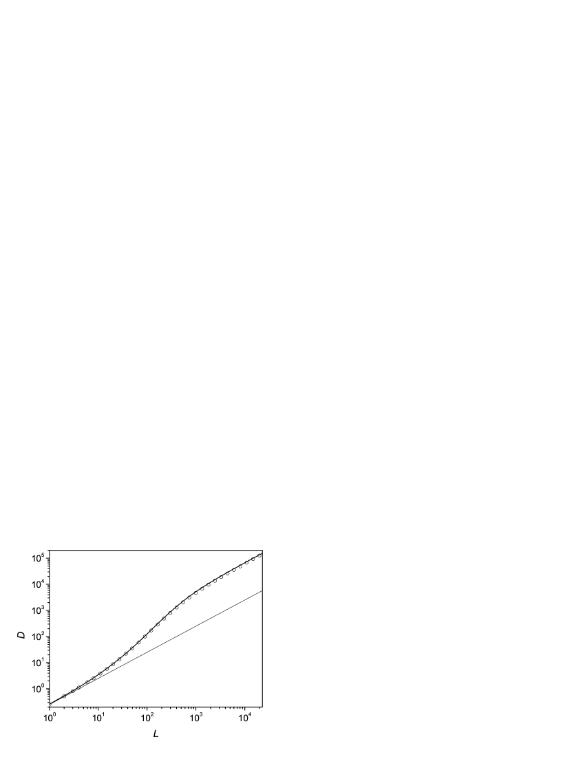
Figure 4: The numerical simulation of the dependence $D(L)$ for the generated sequence with $N=100$ and $\mu=0.4$ (circles). The solid line is the plot of function Eq. (55) with the same values of $N$ and $\mu$.

Note that the above-mentioned phenomenon of the self-similarity relates only to the portion $L<N$ of the curve $D(L)$. Since the decimation procedure leads to the decrease of the parameter $\mu$ (see Eq. (40)), the plot of asymptotics (57) for the reduced sequence at $L\gg N^{\ast}$ goes below the plot for the initial chain.

IV Results of numerical simulations and applications

In this section, we support the obtained above analytical results by numerical simulations of the Markov chain with the conditional probability Eq. (5). Besides, the properties of the studied binary $N$-step Markov chain are compared with ones for the natural objects, specifically for the coarse-grained written and DNA texts.

IV.1 Numerical simulations of the Markov chain

The first stage of the construction of the $N$-step Markov chain was a generation of the initial non-correlated $N$ symbols, zeros and unities, identically distributed with equal probabilities 1/2. Each consequent symbol was then added to the chain with the conditional probability determined by the previous $N$ symbols in accordance with Eq. (5). Than we numerically calculated the variance $D(L)$ by means of Eq. (8). The circles in Fig. 4 represent the calculated variance $D(L)$ for the 100-step Markov chain generated at $\mu=0.4$. A very good agreement between the analytical result in Eq. (55) and the numerical simulation can be observed.

The numerical simulation was also used for the demonstration of the proposition $\spadesuit$ (Fig. 1) and the self-similarity property of the Markov sequence (Fig. 3). The squares in Fig. 3 represent the variance $D(L)$ for the sequence obtained by the stochastic decimation of the initial Markov chain (solid line) where each symbol was omitted with the probability 1/2. The circles in this figure correspond to the regular reduction of the sequence by removing each second symbol.

And finally, the numerical simulations have allowed us to make sure that we are able to determine the parameters $N$ and $\mu$ of a given binary sequence. We generated Markov sequences with different parameters $N$ and $\mu$ and defined numerically the corresponding curves $D(L)$. Then we solved the inverse problem of the reconstruction of the parameters $N$ and $\mu$ by analyzing the curves $D(L)$. The reconstructed parameters were always in a good agreement with their prescribed values. In the next subsections we apply this ability to the treatment of the statistical properties of literary and DNA texts.

IV.2 Literary texts

It is well-known that the statistical properties of the coarse-grained texts written in any language show a remarkable deviation from random sequences schen ; kant . In order to check the applicability of the theory of the binary $N$-step Markov chains to literary texts we resorted to the procedure of coarse graining by the random mapping of all characters of the text onto binary set of symbols, zeros and unities. The statistical properties of the coarse-grained texts depend, but not significantly, on the kind of mapping. This is illustrated by the curves in Fig. 5 where the variance $D(L)$ for five different kinds of the mapping of Bible is presented. Usually, the random mapping leads to nonequal numbers of unities and zeros, $k_{1}$ and $k_{0}$, in the coarse-grained sequence. The particular analysis shows that the variance $D(L)$ (28) gets the additional multiplier,

$$\frac{4k_{0}k_{1}}{(k_{0}+k_{1})^{2}},$$

in this biased case. In order to derive the function $D(L)$ for the non-biased sequence, we divided the numerically calculated value of the variance by this multiplier.

Figure 5: The dependence $D(L)$ for the coarse-grained text of the Bible obtained by means of five different kinds of random mapping.

The study of different written texts has shown that all of them are featured by the pronounced persistent correlations. It is demonstrated by Fig. 6 where five variance curves go significantly higher than the straight line $D=L/4$. However, it should be emphasized that regardless of the kind of mapping the initial portions, $L<80$, of the curves correspond to a slight anti-persistent behavior (see insert to Fig. 7). Moreover, for some inappropriate kinds of mapping (e.g., when all vowels are mapped onto the same symbol) the anti-persistent portions can reach the values of $L\sim 1000$. In order to avoid this problem, all the curves in Fig. 6 are obtained for the definite representative mapping: (a-m) $\rightarrow$ 0; (n-z) $\rightarrow$ 1.

Figure 6: The dependence $D(L)$ for the coarse-grained texts of collection of works on the computer science ($m=2.2\cdot 10^{-3}$, solid line), Bible in Russian ($m=1.9\cdot 10^{-3}$, dashed line), Bible in English ($m=1.5\cdot 10^{-3}$, dotted line), “History of Russians in the 20-th Century” by Oleg Platonov ($m=6.4\cdot 10^{-4}$, dash-dotted line), and “Alice’s Adventures in Wonderland” by Lewis Carroll ($m=2.7\cdot 10^{-4}$, dash-dot-dotted line).

Thus, the persistence is the common property of the binary $N$-step Markov chains and the coarse-grained written texts at large scales. Moreover, the written texts as well as the Markov sequences possess the property of the self-similarity. Indeed, the curves in Fig. 7 obtained from the text of Bible with different levels of the deterministic decimation demonstrate the self-similarity. Presumably, this property is the mathematical reflection of the well-known hierarchy in the linguistics: letters $\rightarrow$ syllables $\rightarrow$ words $\rightarrow$ sentences $\rightarrow$ paragraphs $\rightarrow$ chapters $\rightarrow$ books $\rightarrow$ collected works.

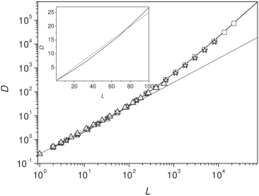
Figure 7: The dependence of the variance $D$ on the tuple length $L$ for the coarse-grained text of Bible (solid line) and for the decimated sequences with different parameters $\lambda$: $\lambda=3/4$ (squares), $\lambda=1/2$ (stars), and $\lambda=1/256$ (triangles). The insert demonstrate the anti-persistent portion of the $D(L)$ plot for Bible.

All the above-mentioned circumstances allow us to suppose that our theory of the binary $N$-step Markov chains can be applied to the description of the statistical properties of the texts of natural languages. However, in contrast to the generated Markov sequence (see Fig. 4) where the full length $\mathcal{M}$ of the chain is far greater than the memory length $N$, the coarse-grained texts described by Fig. 6 are of relatively short length $\mathcal{M}<N$. In other words, the coarse-grained texts are similar not to the Markov chains but rather to some non-stationary short fragments. This implies that each of the written texts is correlated throughout the whole of its length. Therefore, for the written texts, it is impossible to observe the second portion of the curve $D(L)$ parallel (in the log-log scale) to the line $D(L)=L/4$, similar to that shown in Fig. 4. As a result, one cannot define the values of the both parameters $N$ and $\mu$ for the coarse-grained texts. The analysis of the curves in Fig. 6 can give the combination $m=2\mu/N(1-2\mu)$ only (see Eq. (28)). Perhaps, this particular combination is the real parameter governing the persistent properties of the literary texts.

We would like to note that the origin of the long-range correlations in the literary texts is hardly related to the grammatical rules as is claimed in Ref. kant . At short scales $L\leq 80$ where the grammatical rules are in fact applicable the character of correlations is anti-persistent whereas semantic correlations lead to the global persistent behavior of the variance $D(L)$ throughout the whole of literary text.

The numerical estimations of the persistent parameter $m$ and the characterization of the languages and different authors using this parameter can be regarded as a new intriguing problem of the linguistics. For instance, the unprecedented low value of $m$ for the very inventive work by Lewis Carroll as well as the closeness of $m$ for the texts of English and Russian versions of Bible are of certain interest.

It should be noted that there exist special kinds of short-range correlated texts which can be specified by both of the parameters, $N$ and $\mu$. For example, all dictionaries consist of the families of words where some preferable letters are repeated more frequently than in their other parts. Yet another example of the shortly correlated texts is any lexicographically ordered list of words. The analysis of written texts of this kind is given below.

IV.3 Dictionaries

As an example, we have investigated the statistical properties of the coarse-grained alphabetical list of the most frequently used 15462 English words. In contrast to other texts, the statistical properties of the coarse-grained dictionaries are very sensitive to the kind of mapping. If one uses the above-mentioned mapping, (a-m) $\rightarrow$ 0; (n-z) $\rightarrow$ 1, the behavior of the variance $D(L)$ similar to that shown in Fig. 6 would be obtained. The particular construction of the dictionary manifests itself if the preferable letters in the neighboring families of words are mapped onto the different symbols. The variance $D(L)$ for the dictionary coarse-grained by means of such mapping is shown by circles in Fig. 8. It is clearly seen that the graph of the function $D(L)$ consists of two portions similarly to the curve in Fig. 4 obtained for the generated $N$-step Markov sequence. The fitting of the curve in Fig. 8 by the function (55) (solid line in Fig. 8) yielded the values of the parameters $N=180$ and $\mu=0.44$. The parameter $\gamma$ given by Eq. (45) is around 3.9. Note that the characteristic fluctuation length $N(1+\gamma)$ for these $N$ and $\gamma$ is nearly 900. This value corresponds qualitatively to the length of the family of words in the dictionary.

Figure 8: The dependence $D(L)$ for the coarse-grained alphabetical list of 15462 English words (circles). The solid line is the plot of function Eq. (55) with the fitting parameters $N=180$ and $\mu=0.44$.

IV.4 DNA texts

It is known that any DNA text is written by four “characters”, specifically by adenine (A), cytosine (C), guanine (G), and thymine (T). Therefore, there are three nonequivalent types of the DNA text mapping onto one-dimensional binary sequences of zeros and unities. The first of them is the so-called purine-pyrimidine rule, {A,G} $\rightarrow$ 0, {C,T} $\rightarrow$ 1. The second one is the hydrogen-bond rule, {A,T} $\rightarrow$ 0, {C,G} $\rightarrow$ 1. And, finally, the third is {A,C} $\rightarrow$ 0, {G,T} $\rightarrow$ 1.

Figure 9: The dependence $D(L)$ for the coarse-grained DNA text of Bacillus subtilis, complete genome, for three nonequivalent kinds of the mapping. Solid, dashed, and dash-dotted lines correspond to the mappings {A,G} $\rightarrow$ 0, {C,T} $\rightarrow$ 1 (the parameter $m=4.1\cdot 10^{-2}$), {A,T} $\rightarrow$ 0, {C,G} $\rightarrow$ 1 ($m=2.5\cdot 10^{-2}$), and {A,C} $\rightarrow$ 0, {G,T} $\rightarrow$ 1 ($m=1.5\cdot 10^{-2}$), respectively.

By way of example, the variance $D(L)$ for the coarse-grained text of Bacillus subtilis, complete genome (ftp:$//$ftp.ncbi.nih.gov$/$genomes$/$bacteria$/$bacillus_subtilis$/$NC_000964.gbk) is displayed in Fig. 9 for all possible types of mapping. One can see that the persistent properties of DNA are more pronounced than for the written texts and, contrary to the written texts, the $D(L)$ dependence for DNA does not exhibit the anti-persistent behavior at small values of $L$. However, as well as for the written texts, the $D(L)$ curve for DNA does not contain the linear portion given by Eq. (57). This suggests that the DNA chain is not a stationary sequence. In this connection, we would like to point out that the DNA texts represent the collection of extended non-coding regions interrupted by small coding regions (see, for example, prov ). According to Fig. 9, the coding regions do not interrupt the correlation between the non-coding areas, and the DNA system is fully correlated throughout its whole length.

The noticeable deviation of different curves in Fig. 9 from each other demonstrate, in our opinion, that the DNA texts are much more complex objects in comparison with the written ones. Indeed, the different kinds of mapping reveal and emphasize various types of physical attractive correlations between the nucleotides in DNA, such as the strong purine-purine and pyrimidine-pyrimidine persistent correlations (the upper curve), and the correlations caused by a weaker attraction A$\leftrightarrow$T and C$\leftrightarrow$G (the middle curve).

V Conclusion

Thus, we have developed a new approach for the description of the strongly correlated one-dimensional systems. The simple exactly solvable model of the uniform binary $N$-step Markov chain is presented. The memory length $N$ and the parameter $\mu$ of the persistent correlations are two parameters in our theory. Usually, the correlation function ${\cal K}(r)$ is employed as the input characteristics for the description of the correlated random systems. Yet, the function ${\cal K}(r)$ describes not only the direct interconnection of the elements $a_{i}$ and $a_{i+r}$, but also takes into account their indirect interaction via other elements. Since our approach operates with the “origin” parameters $N$ and $\mu$, we believe that it allows us to disclose the intrinsic properties of the system which provide the correlations between the elements.

We have demonstrated the applicability of the suggested theory to the different kinds of correlated stochastic systems. However, there exist some aspects which cannot be interpreted in terms of our two-parameter model. Obviously, more complex models should be developed for the adequate description of real correlated systems.

We acknowledge to Dr. S.V. Denisov who drew our attention to the exposed problem, Yu.L. Rybalko for consultations and kind assistance in the numerical simulations, S.S. Mel’nik and M.E. Serbin for the helpful discussions.

References

- (1) H.E. Stanley et. al., Physica A 224,302 (1996).
- (2) A. Provata and Y. Almirantis, Physica A 247, 482 (1997).
- (3) A. Czirok, R.N. Mantegna, S. Havlin, and H.E. Stanley, Phys. Rev. E52, 446 (1995).
- (4) W. Li, Europhys. Let. 10, 395 (1989).
- (5) R.F. Voss, in: Fundamental Algorithms in Computer Graphics, ed. R.A. Earnshaw (Springer, Berlin, 1985) p. 805.
- (6) M.F. Shlesinger, G.M. Zaslavsky, and J. Klafter, Nature (London) 363, 31 (1993).
- (7) C.V. Nagaev, Theor. Probab. & Appl., 2, 389 (1957) (In Russian).
- (8) I. Kanter and D.F. Kessler, Phys. Rev. Lett. 74, 4559 (1995).
- (9) M.I. Tribelsky, Phys. Rev. Lett. 87, 070201 (2002).
- (10) A. Schenkel, J. Zhang, and Y.C. Zhang, Fractals 1, 47 (1993).