Wavelet Domain Image Separation

Abstract

In this paper, we consider the problem of blind signal and image separation using a sparse representation of the images in the wavelet domain. We consider the problem in a Bayesian estimation framework using the fact that the distribution of the wavelet coefficients of real world images can naturally be modeled by an exponential power probability density function. The Bayesian approach which has been used with success in blind source separation gives also the possibility of including any prior information we may have on the mixing matrix elements as well as on the hyperparameters (parameters of the prior laws of the noise and the sources). We consider two cases: first the case where the wavelet coefficients are assumed to be i.i.d. and second the case where we model the correlation between the coefficients of two adjacent scales by a first order Markov chain. This paper only reports on the first case, the second case results will be reported in a near future The estimation computations are done via a Monte Carlo Markov Chain (MCMC) procedure. Some simulations show the performances of the proposed method.

Keywords.  Blind source separation, wavelets, Bayesian estimation, MCMC Hasting-Metropolis algorithm.

1 Introduction

Blind source separation (BSS) is an active area of research in signal and image processing. Different approaches have been proposed: Principal component analysis (PCA) kn:Tipping99 , Independent factor analysis (IFA) kn:Attias ; kn:Press82 ; kn:PS89 , Independent component analysis (ICA) ProcIEEE ; JADE:NC ; Iscas96-algebra , Maximum likelihood estimation Ziskind88 ; Stoica96 ; Wax91 ; InfoMaxML ; ica99:lacoume ; ica99:oja ; ica99:macleod ; ica99:bermond and Bayesian estimation kn:Rajan97 ; kn:Knuth98 ; kn:Knuth98b ; kn:LeePress ; kn:Roberts98 ; kn:Roberts98 ; kn:Knuth99 ; Lee99a . All these methods use in general independence, sparsity and diversity of the sources either in time or in Fourier domain.

Wavelets, as being a powerful tool of signal processing, have been largely used in many signal processing domains and particularly in signal denoising: abramovich95a ; abramovich98a ; donoho95a ; antoniadis96a ; moulin98a ; simoncelli99a . They have also been used in inverse problems: romberg00a ; wan01a ; donoho92a . The authors in these papers take advantage of the properties of the wavelet coefficients romberg00a : locality, multi-resolution, singularity detection, energy compaction and decorrelation. These outlined properties were said to be primary properties and give rise to what was described to be secondary properties: non-Gaussianity and persistency.

Zibulevsky and Pearlmutter in zibulevsky99a considered the problem of blind source separation within a Bayesian framework using an over-complete sparse representation of the sources. They have, then, minimized an objective function assuming a known noise variance and an empirical estimation of the sources variances.

In this paper, thanks to the unitary property of the wavelet transform, we transport the problem of BSS to the wavelet domain and propose to use the Bayesian estimation framework.

According to the properties romberg00a : decorrelation (the wavelet coefficients of real world signals (images) tend to be approximately decorrelated) and non-Gaussianity (the wavelet coefficients have peaky, heavy tailed marginal distributions), we propose to model the distribution of the wavelet coefficients by a generalized exponential (GE) probability density function (pdf). Thus, independence and sparsity which are the main hypotheses of all the source separation techniques are not required for the sources themselves, but rather for their wavelet coefficients.

The Bayesian approach which has been used with success in blind source separation gives also the possibility of including any prior information we may have on the mixing matrix elements as well as on the hyperparameters (parameters of the prior laws of the noise and the sources) of the problem.

In this work, we make use of the fast wavelet transform developed by Mallat mal99a to have a non-redundant multi-scale representation. This paper is organized as follows: In section 2, we first present the general source separation problem using notation which can be used either in the 1D, 2D or the m-D case. Then, we write the same problem in the wavelet domain and explicit our hypotheses about the prior distributions of the noise and wavelet coefficients. In section 3, we present the Bayesian approach and give the main expressions of the prior and posterior probability density functions. In section 4, first we give the basics of the MCMC algorithm and then apply it to our case. In section 5, we present a few simulation results to show the performances of the proposed method and give some comparison with other known and classical approaches. Finally, in section 6, we present our conclusions and perspectives.

2 Problem Formulation

Blind image separation consists of estimating sources from a set of their linear mixtures. The observations consist of $m$ images $\{X_{i},i=1,\ldots,m\}$ which are instantaneous linear mixtures of $n$ unknown sources $\{S_{j},j=1,\ldots,n\}$, possibly corrupted by additive noise $\{\xi_{i},i=1,\ldots,m\}$:

$$X=AS+\xi$$ (1)

where $A_{(m\times n)}$ is the mixing matrix. To be able to consider 1D, 2D or even m-D signals, we assume that $X_{i}$, $S_{j}$ and $\xi_{i}$ contain each $T$ samples representing either $T$ samples of time series or $T$ pixels of an image or, more generally, $T$ voxels of an m-D signal. Thus, $S$ is a $(n\times T)$ matrix and $X$ and $\xi$ are $(m\times T)$ matrices.

The blind source separation problem is to estimate both the mixing matrix ${\mathb{A}}$ and the sources $S$ from the data $X$ and some assumptions about noise distribution and some prior knowledge of sources distributions. Different approaches have been proposed: Principal component analysis (PCA) hyv01a ; dja99a mainly assumes the problem without noise and Gaussian distribution for sources, Independent component analysis (ICA) hyv01a ; lee98a and Maximum likelihood estimation dja99a assume again the problem without noise but different non-Gaussian distributions for sources, Factor analysis (FA) methods take account of the noise, but assume Gaussian priors both for the noise and the sources.

The Bayesian approach is a generalization of FA with the possibility of any non-Gaussian priors for noise and sources as well as the possibility of accounting for any prior knowledge on the elements of the mixing matrix and the hyperparameters of the problem. In addition, it allows us to jointly estimate the sources $S$, the mixing matrix ${\mathb{A}}$ and even the hyperparameters ${\boldsymbol{\theta}}$ of the problem through the posterior:

$$p(S,{\mathb{A}},{\boldsymbol{\theta}}|X)\propto p(X|S,{\mathb{A}},{\boldsymbol{\theta}})~{}p(S|{\boldsymbol{\theta}})~{}p({\mathb{A}}|{\boldsymbol{\theta}})~{}p({\boldsymbol{\theta}})$$ (2)

We have used this approach before with different priors $p(S|{\boldsymbol{\theta}})$ such as Gaussian Djafari00a and mixture of Gaussians Snoussi00a ; Snoussi00b . We also used this approach in multi-spectral image separation in astronomy for separating the cosmological microwave background (CMB) from other cosmological microwave activities Snoussi01a ; Snoussi01b ; Snoussi01c ; Snoussi01d ; Snoussi01e ; Snoussi01f .

In this paper, we are going to use the same Bayesian approach, but doing the separation taking the advantage of the independence and diversity properties of the wavelet domain coefficients of the sources. Noting by the vector ${\mathb{s}}$ the $T$ samples of one of the sources, by ${\mathb{H}}$ the discrete wavelet transform matrix, and by ${\mathb{w}}$ the complete wavelet coefficients of the 1-D signal we have

$${\mathb{s}}={\mathb{H}}{\mathb{w}}$$ (3)

Now, using the fact that the complete discrete wavelet transform is a linear and unitary operator $({\mathb{H}}^{t}{\mathb{H}}={\mathb{H}}{\mathb{H}}^{t}={\mathb{I}})$, the problem of source separation can be easily transported to the wavelet domain and written as:

$$W_{x}=AW_{s}+W_{\xi}$$ (4)

The main advantage of using this last equation in place of the original source separation problem is that we can more easily assign simple prior laws for $W_{s}$ than for $S$ itself. For example, when $S$ contains discontinuity or non-stationary, still its wavelet coefficients distribution can be modeled by a simple generalized exponential (GE) probability density function (pdf) while it is harder to model appropriately signal samples distribution by a simple pdf. Indeed, it has been reported by many authors that the distribution of the wavelet coefficients of real world images are well modeled by a GE pdf:

$$p(w|\alpha,\beta)={\mathcal{G}}{\mathcal{E}}(\alpha,\beta)=\frac{\beta}{2\alpha\Gamma(1/\beta)}\mbox{exp}\left\{-|w/\alpha|^{\beta}\right\}$$ (5)

Note that $\beta=1$ gives an exponential pdf and $\beta=2$ corresponds to a Gaussian pdf. We are going to use this prior probability law in our Bayesian estimation framework.

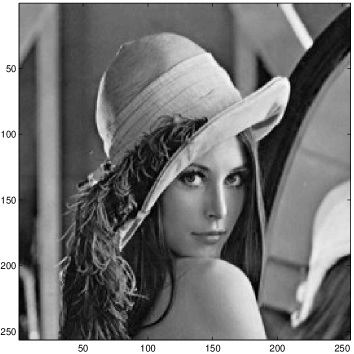
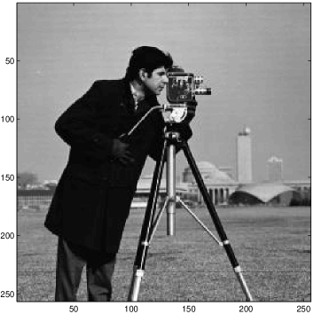
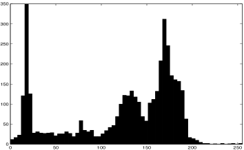
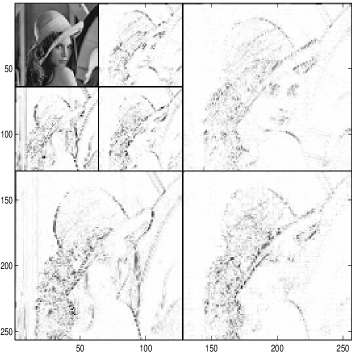
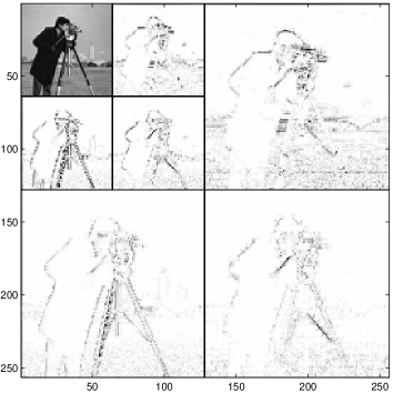
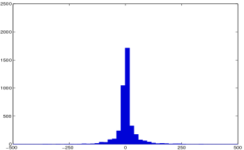
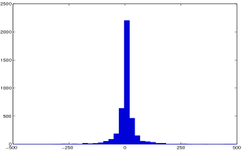
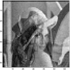
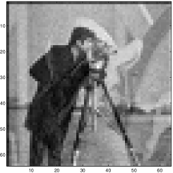
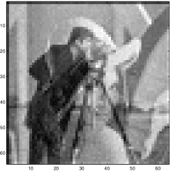
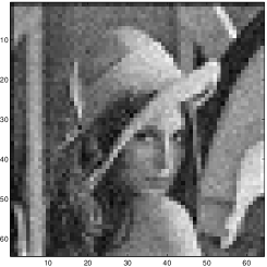
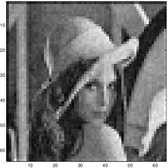
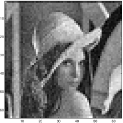
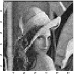
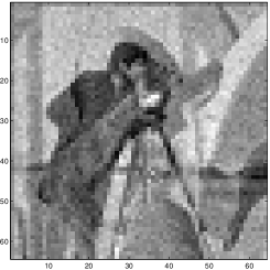
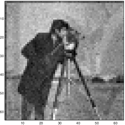
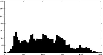
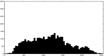
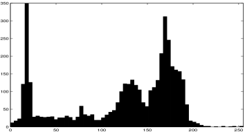
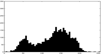
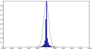
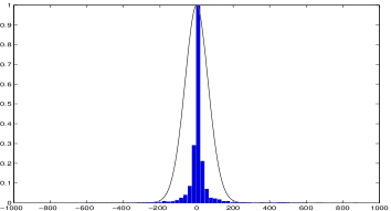
This is shown in the following figures. Figure (1) shows two images (Lena and the cameraman) which we will use later in our simulations. Figure (2) shows their respective histograms while Figure (3) shows their wavelet coefficients and Figure (4) shows the corresponding histograms of their wavelet coefficients. We can remark that even if the histograms of the image pixels are very different, the corresponding wavelet coefficients are similar and can be modeled easily by GE pdf, with different $\alpha\rm{~{}and~{}}\beta$. For a given signal or image, these two parameters can be estimated using either the Maximum Likelihood (ML) method:

$$(\hat{\alpha},\hat{\beta})=\mathop{\mathrm{arg\,min}}_{(\alpha,\beta)}\bigg{(}n\ln\alpha+n\ln\frac{\Gamma(\frac{1}{\beta})}{\beta}+\frac{1}{\alpha^{\beta}}\sum_{i=1}^{n}|x_{i}|^{\beta}\bigg{)}$$

or a moments based method by noting that the moments of the GE pdf are given by:

$${\mathrm{E}}\,{\{x^{n}\}}=\left\{\begin{array}[]{cl}\frac{\Gamma(\frac{n+1}{\beta})}{\Gamma(\frac{1}{\beta})}\alpha^{n}&\textrm{if $n$ is even}\\ \\ 0&\textrm{if $n$ is odd}\end{array}\right.$$

Figure 1: Lena and the cameraman images

Figure 2: Histograms of Lena and the cameraman images

Figure 3: Wavelet coefficients of Lena and the cameraman images

Figure 4: Histograms of the wavelet coefficients of Lena and the cameraman images

3 Bayesian Formulation

In a first step, we assume that the sources and the noise wavelet coefficients are i.i.d. . Thus, to simplify the notation, we denote, respectively, by ${\mathb{x}}(k)$, ${\mathb{s}}(k)$ and ${\boldsymbol{\xi}}(k)$ the vectors containing the wavelet coefficients of the data, the sources and the noise for a given index $k$. Thus, we have ${\mathb{x}}(k)={\mathb{A}}{\mathb{s}}(k)+{\boldsymbol{\xi}}(k)$. Hereafter, we omit the index $k$ and note it only when needed. To proceed with the Bayesian approach, we have to assign the prior laws. In the following we assume:

• The noise wavelet coefficients ${\boldsymbol{\xi}}$ are assumed independent and $p(\xi_{i})={\mathcal{G}}{\mathcal{E}}(\alpha_{\epsilon_{i}},\beta)$. Then

  $$p({\mathb{x}}|{\mathb{A}},{\mathb{s}},\{\alpha_{\epsilon_{i}},\beta\})=\prod_{i=1}^{m}\left(\frac{\beta}{2\alpha_{\epsilon_{i}}\Gamma(1/\beta)}\right)\mbox{exp}\left\{-\sum_{i=1}^{m}\big{(}|x_{i}-[{\mathb{A}}{\mathb{s}}]_{i}|/\alpha_{\epsilon_{i}}\big{)}^{\beta}\right\}$$ (6)

• The wavelet coefficients ${\mathb{s}}$ of the sources are also assumed independent and $p(s_{j})={\mathcal{G}}{\mathcal{E}}(\alpha_{s_{j}},\beta_{s})$. Then

  $$p({\mathb{s}}|\left\{\alpha_{s_{j}},\beta_{s}\right\})=\prod_{j=1}^{n}\left(\frac{\beta_{s}}{2\alpha_{s_{j}}\Gamma(1/\beta_{s})}\right)\mbox{exp}\left\{-\sum_{j=1}^{n}\big{(}|s_{j}|/\alpha_{s_{j}}\big{)}^{\beta_{s}}\right\}$$ (7)

• The elements $a_{ij}$ of the mixing matrix ${\mathb{A}}$ are assumed i.i.d. and Gaussian with mean values $\mu_{ij}$ and variances $\sigma_{ij}^{2}$:

  $$p(a_{ij})=(2\pi\sigma_{a_{ij}}^{2})^{-1/2}\mbox{exp}\left\{-\frac{1}{{2\sigma_{a_{ij}}^{2}}}(a_{ij}-\mu_{ij})^{2}\right\}$$ (8)

  Therefore, we may note by

  $$p({\mathb{A}}|{\mathb{M}},{\mathb{R}}_{a}) = (2\pi)^{-{mn}/2}|{\mathb{R}}_{a}|^{-1/2}$$ (9)

  $$\exp\left\{-\frac{1}{2}\big{(}\textrm{Vect}({\mathb{A}}-{\mathb{M}})\big{)}^{t}{\mathb{R}}_{a}^{-1}\big{(}\textrm{Vect}({\mathb{A}}-{\mathb{M}})\big{)}\right\}$$

  where ${\mathb{M}}=\left\{\mu_{ij}\right\}$, $\textrm{Vect}({\mathb{M}})$ means a vector containing the elements of the matrix ${\mathb{M}}$ and

  $${\mathb{R}}_{a~{}(mn\times mn)}=\mbox{diag}({\sigma_{a_{11}}^{2}},{\sigma_{a_{12}}^{2}},\ldots,{\sigma_{a_{mn}}^{2}})$$

• All the hyperparameters $(\frac{1}{\alpha_{\epsilon_{i}}^{\beta}},\frac{1}{\alpha_{s_{j}}^{\beta_{s}}})$ are assumed independent and assigned standard Gamma prior distributions $p(x)={\mathcal{G}}(2,1)$, where:

  $${{\mathcal{G}}}(x|a,b)=\frac{x^{a-1}}{b^{a}\Gamma(a)}\exp(-\frac{x}{b})$$ (10)

The joint a posteriori law of the sources coefficients ${\mathb{s}}$, the mixing matrix ${\mathb{A}}$ and the hyperparameters ${\boldsymbol{\theta}}$ is then given by:

$$p({\mathb{s}},{\mathb{A}},{\boldsymbol{\theta}}|{\mathb{x}})\propto p({\mathb{x}}|{\mathb{s}},{\mathb{A}},{\boldsymbol{\theta}})~{}p({\mathb{s}}|{\boldsymbol{\theta}})~{}p({\mathb{A}}|{\boldsymbol{\theta}})~{}p({\boldsymbol{\theta}})$$ (11)

where we noted all the hyperparameters $\left({1\over\alpha_{\epsilon_{i}}^{\beta}},{1\over\alpha_{s_{j}}^{\beta_{s}}}\right)$ by ${\boldsymbol{\theta}}$.

The conditional a posteriori laws of ${\mathb{s}},{\mathb{A}}$ and ${\boldsymbol{\theta}}$ are then given by :

$$p({\mathb{s}}|{\mathb{x}},{\mathb{A}},{\boldsymbol{\theta}}) \propto \prod_{i=1}^{m}\left(\frac{\beta}{2\alpha_{\epsilon_{i}}\Gamma(1/\beta)}\right)~{}\prod_{j=1}^{n}\left(\frac{\beta_{s}}{2\alpha_{s_{j}}\Gamma(1/\beta_{s})}\right)$$ (12)

$$\mbox{exp}\left\{-\sum_{i=1}^{m}\big{(}{|x_{i}-[{\mathb{A}}{\mathb{s}}]_{i}|/\alpha_{\epsilon_{i}}}\big{)}^{\beta}-\sum_{j=1}^{n}\big{(}{|s_{j}|/\alpha_{s_{j}}}\big{)}^{\beta_{s}}\right\}$$

$$p({\mathb{A}}|{\mathb{x}},{\mathb{s}},{\boldsymbol{\theta}}) \propto \prod_{i=1}^{m}\left(\frac{\beta}{2\alpha_{\epsilon_{i}}\Gamma(1/\beta)}\right)~{}(2\pi)^{-{mn}/2}|{\mathb{R}}_{a}|^{-1/2}$$ (13)

$$\mbox{exp}\left\{-\sum_{i=1}^{m}\big{(}{|x_{i}-[{\mathb{A}}{\mathb{s}}]_{i}|/\alpha_{\epsilon_{i}}}\big{)}^{\beta}\right\}$$

$$\mbox{exp}\left\{-\frac{1}{2}\big{(}\textrm{Vect}({\mathb{A}}-{\mathb{M}})\big{)}^{t}{\mathb{R}}_{a}^{-1}\big{(}\textrm{Vect}({\mathb{A}}-{\mathb{M}})\big{)}\right\}$$

$$p\bigg{(}\theta_{i}={1\over\alpha_{\epsilon_{i}}^{\beta}}|{\mathb{x}},{\mathb{s}},{\mathb{A}}\bigg{)} \propto \left(\frac{\beta}{2\Gamma(1/\beta)}\right)^{K}\left(\frac{1}{\alpha_{\epsilon_{i}}^{\beta}}\right)^{{K\over\beta}+1}$$ (14)

$$\mbox{exp}\left\{{1\over\alpha_{\epsilon_{i}}^{\beta}}\left(-\sum_{k=1}^{K}{|x_{i}(k)-[{\mathb{A}}{\mathb{s}}(k)]_{i}|}^{\beta}+1\right)\right\}$$

$$p\bigg{(}\theta_{j}={1\over\alpha_{s_{j}}^{\beta_{s}}}|{\mathb{x}},{\mathb{s}},{\mathb{A}}\bigg{)} \propto \left(\frac{\beta_{s}}{2\Gamma(1/\beta_{s})}\right)^{K}\left(1\over\alpha_{s_{j}}^{\beta_{s}}\right)^{{K\over\beta_{s}}+1}$$ (15)

$$\mbox{exp}\left\{{1\over\alpha_{s_{j}}^{\beta_{s}}}\left(-\sum_{k=1}^{K}{|s_{j}(k)|}^{\beta_{s}}+1\right)\right\}$$

4 MCMC Implementation

Once the expression of the joint a posteriori law $p({\mathb{s}},{\mathb{A}},{\boldsymbol{\theta}}|{\mathb{x}})$ of all the unknowns has been derived, we can use it to infer them. However, in general, the computation of the normalization factor needs a huge dimensional integration. When the MAP estimation is chosen, this normalization factor is not needed, but it is formally needed for other estimation rules such as the posterior mean. The MCMC algorithms are then the basic tools to generate samples from the posterior law. The main idea is to generate successively the samples from the posterior laws ${\mathb{s}}^{(k)}\sim p({\mathb{s}}|{\mathb{A}}^{(k)},{\boldsymbol{\theta}}^{(k)},{\mathb{x}})$, ${\mathb{A}}^{(k)}\sim p({\mathb{A}}|{\mathb{s}}^{(k)},{\boldsymbol{\theta}}^{(k)},{\mathb{x}})$ and ${\boldsymbol{\theta}}^{(k)}\sim p({\boldsymbol{\theta}}|{\mathb{s}}^{(k)},{\mathb{A}}^{(k)},{\mathb{x}})$ and then estimate their expected values by averaging these samples.

We use the Hasting-Metropolis algorithm combined to a Gibbs sampler to obtain an ergodic chain, and then approximate the ensemble expectation of any quantity $Z$ by its empirical mean:

$${\mathrm{E}}\,{(Z)}\approx\frac{1}{(N-T+1)}\sum_{t=T}^{N}h(Z^{(t)})$$

where $\{Z^{(t)}\}$ are samples from $p(z|.)$.

Noting that, when $\beta=2$ and $\beta_{s}=2$, the posterior laws for the sources and for the elements of the mixing matrix are Gaussian, we can use these Gaussian as the trial (or instrumental) pdf. Thus, to simplify the presentation of the proposed algorithm, we give here the expressions of these Gaussian posterior laws:

• The trial posterior pdf of the sources is Gaussian $g({\mathb{s}}|{\boldsymbol{\theta}},{\mathb{x}})={\mathcal{N}}(\widehat{{\mathb{s}}},\widehat{{\mathb{R}}}_{s})$ with

  $$\widehat{{\mathb{s}}}=2\widehat{{\mathb{R}}}_{s}{\mathb{A}}^{t}{\mathb{R}}_{\alpha_{\epsilon}}^{-1}{\mathb{x}}$$ (16)

  and

  $$\widehat{{\mathb{R}}}_{s}={1\over 2}({\mathb{A}}^{t}{\mathb{R}}_{\alpha_{\epsilon}}^{-1}{\mathb{A}}+{\mathb{R}}_{\alpha_{s}}^{-1})^{-1}$$ (17)

  where

  $${\mathb{R}}_{\alpha_{s}~{}(n\times n)} = \mbox{diag}({\alpha_{s_{1}}^{2}},{\alpha_{s_{2}}^{2}},\ldots,{\alpha_{s_{n}}^{2}})$$

  $${\mathb{R}}_{\alpha_{\epsilon}~{}(m\times m)} = \mbox{diag}({\alpha_{\epsilon_{1}}^{2}},{\alpha_{\epsilon_{2}}^{2}},\ldots,{\alpha_{\epsilon_{m}}^{2}})$$

• The trial posterior pdf of the mixing matrix elements is Gaussian $g(\textrm{Vect}({\mathb{A}})|{\boldsymbol{\theta}},{\mathb{x}})={\mathcal{N}}(\textrm{Vect}(\widehat{{\mathb{M}}}),\widehat{{\mathb{R}}}_{a})$ with

  $$\textrm{Vect}(\widehat{{\mathb{M}}})=\widehat{{\mathb{R}}}_{a}\left(2\textrm{Vect}({\mathb{s}}{\mathb{x}}^{t}{\mathb{R}}_{\alpha_{\epsilon}}^{-1})+{\mathb{R}}_{a}^{-1}\textrm{Vect}({\mathb{M}})\right)$$ (18)

  and

  $$\widehat{{\mathb{R}}}_{a}=\left(2\left({\mathb{E}}^{t}{\mathb{R}}_{\alpha_{\epsilon}}^{-1}{\mathb{E}}\right).*{\mathb{C}}+{\mathb{R}}_{a}^{-1}\right)^{-1}$$ (19)

  where

  $${\mathb{E}}_{(m\times mn)} = \textrm{blockdiag}\left([1,\ldots,1]_{(n\times 1)},m\right)$$

  $${\mathb{C}}_{(mn\times mn)} = \textrm{blockdiag}\left(ss^{t}_{(n\times n)},m\right)$$

  where blockdiag$({\mathb{M}},m)$ stands for a $m$ block-diagonal matrix with matrix ${\mathb{M}}$ as the block elements, and ${\mathb{A}}.*{\mathb{B}}$ stands for a point-wise multiplication of two matrices, i.e. ${\mathb{C}}={\mathb{A}}.*{\mathb{B}}$ means ${\mathb{C}}_{ij}={\mathb{A}}_{ij}{\mathb{B}}_{ij}$.

The proposed MCMC algorithm is then the following:

• Initialize ${\mathb{s}},{\mathb{A}},{\boldsymbol{\theta}}$  to  ${\mathb{s}}^{0},{\mathb{A}}^{0},{\boldsymbol{\theta}}^{0}$ and repeat the following steps until convergence

• Sampling ${\mathb{s}}(k)$, for $k=1\ldots K$:

  $${\mathb{z}}\leadsto g({\mathb{z}}|{\boldsymbol{\theta}},{\mathb{x}})={\mathcal{N}}(\widehat{{\mathb{s}}},\widehat{{\mathb{R}}}_{s})$$

  where $\widehat{{\mathb{s}}}$ and $\widehat{{\mathb{R}}}_{s}$ are given, respectively by eq. (16) and eq. (17) and

  $${\mathb{s}}^{(t+1)}(k)=\left\{\begin{array}[]{cll}{\mathb{z}}&\textrm{with probability}&\rho\\ {\mathb{s}}^{(t)}(k)&\textrm{with probability}&1-\rho\end{array}\right.$$

  with

  $$\rho=\textrm{min}\left(1,\frac{p({\mathb{z}}|{\mathb{x}}(k),{\mathb{A}},{\boldsymbol{\theta}})}{p({\mathb{s}}^{(t)}(k)|{\mathb{x}}(k),{\mathb{A}},{\boldsymbol{\theta}})}\bigg{/}\frac{g({\mathb{z}})}{g({\mathb{s}}^{(t)}(k))}\right)$$

  where $p({\mathb{z}}|{\mathb{x}}(k),{\mathb{A}},{\boldsymbol{\theta}})$ is given by eq.(12).

• Sampling ${\mathb{A}}$:

  $${\mathb{z}}\leadsto g({\mathb{z}}|{\boldsymbol{\theta}},{\mathb{x}})={\mathcal{N}}(\textrm{Vect}(\widehat{{\mathb{M}}}),\widehat{{\mathb{R}}}_{a})$$

  where $\widehat{{\mathb{M}}}$ and $\widehat{{\mathb{R}}}_{a}$ are given, respectively by eq. (18) and eq. (19) and

  $${\mathb{A}}^{(t+1)}=\left\{\begin{array}[]{cll}\textrm{Mat}({\mathb{z}})&\textrm{with probability}&\rho\\ {\mathb{A}}^{(t)}&\textrm{with probability}&1-\rho\end{array}\right.$$

  with

  $$\rho=\textrm{min}\left(1,\frac{p({\mathb{z}}|{\mathb{x}},{\mathb{s}},{\boldsymbol{\theta}})}{p(\textrm{Vect}({\mathb{A}}^{(t)})|{\mathb{x}},{\mathb{s}},{\boldsymbol{\theta}})}\bigg{/}\frac{g({\mathb{z}})}{g(\textrm{Vect}({\mathb{A}}^{(t)}))}\right)$$

  where $p({\mathb{z}}|{\mathb{x}}(k),{\mathb{A}},{\boldsymbol{\theta}})$ is given by eq. (13).

• Sampling $\theta_{i}=\frac{1}{\alpha_{\epsilon_{i}}^{\beta}}$, for $i=1\ldots m$:

  $${\boldsymbol{\theta}}^{(t+1)}\leadsto{\mathcal{G}}(a,b)$$

  with

  $$a=\frac{K}{\beta}+2\mbox{~{}~{}~{}and~{}~{}~{}}b=\left(\sum_{k=1}^{K}|x_{i}(k)-[{\mathb{A}}{\mathb{s}}(k)]_{i}|^{\beta}+1\right)^{-1}$$

• Sampling $\theta_{j}=\frac{1}{\alpha_{s_{j}}^{\beta_{s}}}$, for $j=1\ldots n$:

  $${\boldsymbol{\theta}}_{j}^{(t+1)}\leadsto{\mathcal{G}}(a,b)$$

  with

  $$a=\frac{K}{\beta_{s}}+2\mbox{~{}~{}~{}and~{}~{}~{}}b=\Big{(}\sum_{k=1}^{K}|s_{j}(k)|^{\beta_{s}}+1\Big{)}^{-1}.$$

5 Simulation results

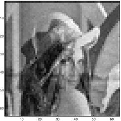
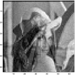
To illustrate the performances of the proposed method, we consider two cases: a favorable case where we have 2 unknown sources with 3 measured data, and a more difficult case where we have only two measured data. In the first case, we consider $64\times 64$ pixel images of the two images of Figure (1) with the following rectangular mixing matrix:

$$A=\left[\begin{array}[]{cc}0.8211&0.4053\\ 0.3769&0.7997\\ 0.4287&0.4428\end{array}\right]$$

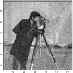
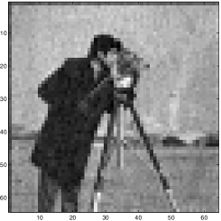
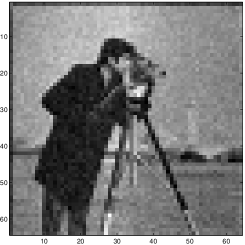
to generate the mixed images and added a white Gaussian noise of zero mean to obtain the data with a SNR $=30$dB, where SNR is defined as being the ratio of the mixed signal energy to that of the noise in dB: $\textrm{SNR}_{\textrm{dB}}=10\log_{10}\left({\|{\mathb{x}}\|^{2}\over\|{\boldsymbol{\epsilon}}\|^{2}}\right)$. Figure (5) shows the mixed images obtained.

Figure 5: The mixed images in the rectangular case

We applied the proposed method directly on the mixed images where we assumed noise to be i.i.d. and original images to be independent and Gaussian. Then, we accounted for the local correlation between neighboring pixels through a Markovian modeling of the original images. Finally, we applied the method in the wavelet domain. Figure (6) shows the separated images obtained for each case.

(a)	(b)	(c)
PSNR = $0.0910$	PSNR = $0.0651$	PSNR = $0.1144$
PSNR = $0.1712$	PSNR = $0.1049$	PSNR = $0.1306$

Figure 6: Estimated source images : (a) Sources assumed independent, (b) Accounting for local correlation in the sources, (c) Estimated sources obtained in the wavelet domain.

We may note that in this case which is an extremely favorable case the three different methods give satisfactory results and it is not easy to really distinguish between these three methods as it can also be noted from the PSNR’s of the reconstructed images compared to the original images. We can, however, speculate that accounting for local correlation of the image pixels outperforms the other two methods.

We have also considered a second case where we have an equal number of measurements and sources (square case). The original source images where mixed with the following matrix:

$$A=\left[\begin{array}[]{cc}0.9088&0.4928\\ 0.4172&0.8702\end{array}\right]$$

and the same type of noise was added to obtained the data with a SNR = $30$dB shown in Figure (7).

Figure 7: The mixed images for the case of a square mixing matrix

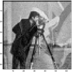Figure (8) shows the reconstructed images by the three methods of modeling the source images, i.e. Gaussian i.i.d. , Gauss-Markov on pixels and GE on their wavelet coefficients.

(a)	(b)	(c)
PSNR = $0.2560$	PSNR = $0.0740$	PSNR = $0.1260$
PSNR = $0.3150$	PSNR = $0.0998$	PSNR = $0.1660$

Figure 8: Estimated source images : (a) Sources assumed independent, (b) Accounting for local correlation in the sources, (c) Estimated sources obtained in the wavelet domain.

We should point out that we have used the following values for the initialization of the algorithm:

$${\mathb{A}}^{(0)}=\left[\begin{array}[]{cc}1.0&0.0\\ 0.0&1.0\end{array}\right],\quad\sigma^{2^{(0)}}=\sigma_{1}^{2^{(0)}}=\sigma_{2}^{2^{(0)}}=1\longrightarrow\left\{\begin{array}[]{l}\alpha_{\epsilon_{i}}^{(0)}=\sqrt{2}~{},~{}\beta=2\\ \alpha_{s_{j}}^{(0)}=(2)^{1/\beta_{s}}~{},~{}\beta_{s}=1.9\end{array}\right.$$

The final estimated values obtained by averaging the last 10% samples after 5000 iterations are the following:

$$\left.\begin{array}[]{cc}\widehat{{\mathb{A}}}=\left[\begin{array}[]{cc}0.8604&0.4681\\ 0.5096&0.8837\end{array}\right]&\begin{array}[]{l}\hat{\alpha}_{\epsilon_{1}}=24.0966,~{}\hat{\alpha}_{\epsilon_{2}}=24.2096\\ \hat{\alpha}_{s_{1}}=91.4272,~{}\hat{\alpha}_{s_{2}}=83.5939\end{array}\end{array}\right.$$

We may also note that the estimated values of $\alpha_{\epsilon_{1}}$, $\alpha_{\epsilon_{2}}$, $\alpha_{s_{1}}$ and $\alpha_{s_{2}}$ directly from the original images are:

$\alpha_{\epsilon_{1}}=7.6457,~{}\alpha_{\epsilon_{2}}=7.2784$

$\alpha_{s_{1}}=96.5342,~{}\alpha_{s_{2}}=107.9316$

We notice that neither the noise variances nor the variance of the second image (the cameraman) were well estimated. We clearly notice that in Figure (8). However, the separation of the images in the wavelet domain outperforms the separation applied directly to the images assuming sources to be independent and this is due to the decorrelation property of the wavelet transform. In fact, the wavelet transform nearly decorrelates a signal, thus assuming independent wavelet coefficients is more realistic than assuming independent signal samples.

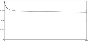
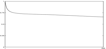
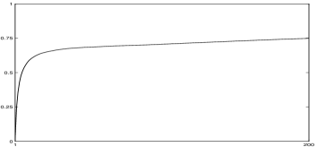
Figure (9) shows the rate of acceptance of the generated samples from the Gaussian to approximate the posterior law of the wavelet coefficients for $\beta_{s}=1.9$.

Figure 9: Rate of acceptance of the samples for the wavelet coefficients along the iterations

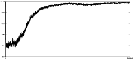
We also noticed that this rate of acceptance is a function of the parameter $\beta_{s}$:

$$\rho\searrow 0~{}~{}~{}~{}\textrm{as}~{}~{}~{}~{}\beta_{s}\searrow 1$$

and

$$\rho\nearrow 1~{}~{}~{}~{}\textrm{as}~{}~{}~{}~{}\beta_{s}\nearrow 2$$

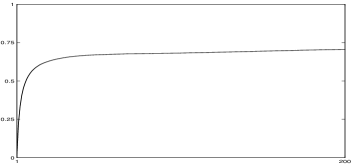
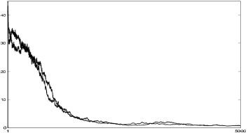
Figure (10) shows the convergence of the elements of the matrix ${\mathb{A}}$ and Figure (11) shows the convergence of the hyperparameters.

$a_{11}$	$a_{12}$
$a_{21}$	$a_{22}$

Figure 10: Convergence of the elements of ${\mathb{A}}$ during the first $200$ iterations

$\alpha_{\epsilon}$	$\alpha_{s}$

Figure 11: Convergence of the hyperparameters ${\boldsymbol{\theta}}$: Left: $\alpha_{\epsilon 1}$ and $\alpha_{\epsilon 2}$  Right: $\alpha_{s1}$ and $\alpha_{s2}$.

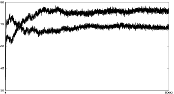Figure (12) shows the histograms of the original and estimated images while Figure (13) shows the histograms of the wavelet coefficients of the original images superposed with the Exponential pdf with parameter $\alpha$ estimated with the algorithm.

(a)	(b)

Figure 12: The histogram of: (a) Original source images, (b) The estimated images (top: Lena image, bottom: The cameraman image)

(a)	(b)

Figure 13: The histogram of the wavelet coefficients of the original source images superposed with the pdf of the estimated images of: (a) Lena image, (b) The cameraman image

6 Conclusions and Perspectives

In this contribution we proposed an approach to jointly estimate the mixing matrix and the original source images. We transported the problem to the wavelet domain using a Bayesian approach where the wavelet coefficients of real world images are naturally modeled by generalized exponential distributions. Independence of the wavelet coefficients of signals is more realistic than the independence of the signals themselves.

In a first step, we assumed all the wavelet coefficients to be independent and identically distributed and follow a GE pdf with a fixed value for its parameter $\beta_{s}$ while its second parameter is estimated during the iterations. Even if this gives satisfactory results, it will be better to estimate $\beta_{s}$ too during the iterations.

A second point is that the choice of a Gaussian trial pdf is good when $\beta_{s}$ is not far from $2$, but it seems that this choice is no more efficient when $\beta_{s}$ approaches $1$.

Finally, since the wavelet coefficients of real world signals (images) tend to propagate through scales, a future work is to put a Markovian model on the wavelet coefficients taking into account inter-scale correlation of the coefficients.

References

- (1) M. E. Tipping and C. M. Bishop, “Mixtures of probabilistic principal components analysis,” Neural Computation, vol. 11, pp. 443–482, 1999.
- (2) H. Attias, “Independent factor analysis,” Neural Computation, vol. 11, pp. 803–851, 1999.
- (3) S. J. Press, Applied Multivariate Analysis: Using Bayesian and Frequentist Methods of Inference. Malabar, Florida: Robert E. Krieger Publishing Company, 1982.
- (4) S. J. Press and K. Shigemasu, “Bayesian inference in factor analysis,” in Contributions to Probability and Statistics, ch. 15, Springer-Verlag, 1989.
- (5) J.-F. Cardoso, “Blind signal separation: statistical principles,” Proceedings of the IEEE. Special issue on blind identification and estimation, pp. 2009–2025, octobre 1998.
- (6) J.-F. Cardoso, “High-order contrasts for independent component analysis,” Neural Computation, vol. 11, pp. 157–192, janvier 1999.
- (7) J.-F. Cardoso and P. Comon, “Independent component analysis, a survey of some algebraic methods,” in Proc. ISCAS’96, vol. 2, pp. 93–96, 1996.
- (8) I. Ziskind and M. Wax, “Maximum likelihood localization of multiple sources by alternating projection,” IEEE Trans. Acoust. Speech, Signal Processing, vol. ASSP-36, pp. 1553–1560, octobre 1988.
- (9) P. Stoica, B. Ottersten, M. Viberg, and R. L. Moses, “Maximum likelihood array processing for stochastic coherent sources,” Signal Processing, vol. 44, pp. 96–105, janvier 1996.
- (10) M. Wax, “Detection and localization of multiple sources via the stochastic signals model,” IEEE Trans. Signal Processing, vol. 39, pp. 2450–2456, novembre 1991.
- (11) J.-F. Cardoso, “Infomax and maximum likelihood for source separation,” IEEE Letters on Signal Processing, vol. 4, pp. 112–114, avril 1997.
- (12) J.-L. Lacoume, “A survey of source separation,” in Proc. First International Conference on Independent Component Analysis and Blind Source Separation ICA’99, (Aussois, France), pp. 1–6, January 11–15, 1999.
- (13) E. Oja, “Nonlinear PCA criterion and maximum likelihood in independent component analysis,” in Proc. First International Conference on Independent Component Analysis and Blind Source Separation ICA’99, (Aussois, France), pp. 143–148, January 11–15, 1999.
- (14) R. B. MacLeod and D. W. Tufts, “Fast maximum likelihood estimation for independent component analysis,” in Proc. First International Conference on Independent Component Analysis and Blind Source Separation ICA’99, (Aussois, France), pp. 319–324, January 11–15, 1999.
- (15) O. Bermond and J.-F. Cardoso, “Approximate likelihood for noisy mixtures,” in Proc. First International Conference on Independent Component Analysis and Blind Source Separation ICA’99, (Aussois, France), pp. 325–330, January 11–15, 1999.
- (16) J. J. Rajan and P. J. W. Rayner, “Decomposition and the discrete karhunen-loeve transformation using a bayesian approach,” IEE Proceedings - Vision, Image, and Signal Processing, vol. 144, no. 2, pp. 116–123, 1997.
- (17) K. Knuth, “Bayesian source separation and localization,” in SPIE’98 Proceedings: Bayesian Inference for Inverse Problems, San Diego, CA (A. Mohammad-Djafari, ed.), pp. 147–158, July 1998.
- (18) K. Knuth and H. Vaughan JR., “Convergent Bayesian formulation of blind source separation and and electromagnetic source estimation,” in MaxEnt 98 Proceedings: Int. Workshop on Maximum Entropy and Bayesian methods, Garching, Germany (F. R. von der Linden W., Dose W. and P. R., eds.), p. in press, 1998.
- (19) S. E. Lee and S. J. Press, “Robustness of Bayesian factor analysis estimates,” Communications in Statistics – Theory And Methods, vol. 27, no. 8, 1998.
- (20) S. J. Roberts, “Independent component analysis: Source assessment, and separation, a Bayesian approach,” IEE Proceedings - Vision, Image, and Signal Processing, vol. 145, no. 3, 1998.
- (21) K. Knuth, “A Bayesian approach to source separation,” in Proceedings of the First International Workshop on Independent Component Analysis and Signal Separation: ICA’99, Aussios, France (C. J. J.-F. Cardoso and P. Loubaton, eds.), pp. 283–288, 1999.
- (22) T. Lee, M. Lewicki, M. Girolami, and T. Sejnowski, “Blind source separation of more sources than mixtures using overcomplete representation,” IEEE Signal Processing Letters, p. in press, 1999.
- (23) F. Abramovich and Y. Benjamini, “Thresholding of wavelets coefficients as multiples hypotheses testing procedure,” Wavelets and Statistics, A. Antoniadis and G. Oppenheim Eds, Lecture Notes in Statistics, pp. 5–14, 1995.
- (24) F. A. T. Sapatinas and B. Silverman, “Wavelet thresholding via a bayesian approach,” The Royal Statiscal Society B, no. 60, pp. 725–749, 1998.
- (25) D. L. Donoho, “De-noising by soft-thresholding,” IEEE Trans. Inf. Theory, 1995.
- (26) A. Antoniadis, D. Leporini, and J. Pesquet, “Wavelet Thresholding for some classes of Non-Gaussian Noise,” Satistica Neerlandica, 2000.
- (27) P. Moulin and J. Liu, “Analysis of multiresolution image denoising schemes using generalized-gaussian and complexity priors,” IEEE Transactions on Information Theory, April 1999.
- (28) E. P. Simoncelli, “Bayesian Denoising of Visual Images in the Wavelet Domain,” Lecture Notes in Statistics, vol. 141, pp. 291–308, March, 30 1999.
- (29) J. K. Romberg, H. Choi, and R. G. Baraniuk, “Bayesian Tree-Structured Image Modeling using Wavelet-domain Hidden Markov Models,” IEEE Transactions on Image Processing, March 2000.
- (30) Y. Wan and R. D. Nowak, “A Multiscale Bayesian Framework for Linear Inverse Problems and Its Application to Image Restoration,” IEEE Transactions on Image Processing, January 2001.
- (31) D. L. Donoho, “Nonliner Solution of Linear Inverse Problems by Wavelet-Vaguelette Decomposition,” IEEE Transactions on Signal Processing, April 1992.
- (32) M. Zibulevsky and B. A. Pearlmutter, “Blind Source Separation by Sparse Decomposition,” tech. rep., Computer Science Dept, FEC 313, University of Mexico, Albuquerque, NM 87131 USA, July 19 1999.
- (33) S. Mallat, a Wavelet Tour of Signal Processing. Academic Press, 1999.
- (34) A. Hyvrinen, J. Karhunen, and E. Oja, Independant Component Analysis. John Wiley & Sons Inc., 2001.
- (35) A. Mohammad-Djafari, “A Bayesian Approach to Source Sepration,” (Boise, Idaho, USA), 19th Int. workshop on Bayesian and Maximum Entropy methods, MaxEnt, 1999.
- (36) T.-W. Lee, Independant Component Analysis ”Theory and Applications”. Boston, Dordrecht, London: Kluwer Academic Publishers, 1998.
- (37) A. Mohammad-Djafari, “Bayesian inference and maximum entropy methods,” in Bayesian Inference and Maximum Entropy Methods (A. Mohammad-Djafari, ed.), (Gif-sur-Yvette), MaxEnt Workshops, à paraître dans Amer. Inst. Physics, juillet 2000.
- (38) H. Snoussi and A. Mohammad-Djafari, “Bayesian source separation with mixture of gaussians prior for sources and gaussian prior for mixture coefficients,” in Bayesian Inference and Maximum Entropy Methods (A. Mohammad-Djafari, ed.), (Gif-sur-Yvette), pp. 388–406, Proc. of MaxEnt, Amer. Inst. Physics, juillet 2000.
- (39) H. Snoussi and A. Mohammad-Djafari, “Approche bayésienne pour la séparation de sources,” rapport de stage de dea-ats, gpi–l2s, 2000.
- (40) H. Snoussi and A. Mohammad-Djafari, “Dégénérescences des estimateurs MV en séparation de sources,” technical report ri-s0010, gpi–l2s, 2001.
- (41) H. Snoussi and A. Mohammad-Djafari, “Séparation de sources par une approche bayésienne hiérarchique,” in Actes 18e coll. GRETSI, (Toulouse), septembre 2001.
- (42) H. Snoussi and A. Mohammad-Djafari, “Penalized maximum likelihood for multivariate gaussian mixture,” in Bayesian Inference and Maximum Entropy Methods (R. L. Fry, ed.), pp. 36–46, MaxEnt Workshops, Amer. Inst. Physics, août 2002.
- (43) H. Snoussi and A. Mohammad-Djafari, “Bayesian separation of HMM sources,” in Bayesian Inference and Maximum Entropy Methods (R. L. Fry, ed.), pp. 77–88, MaxEnt Workshops, Amer. Inst. Physics, août 2002.
- (44) H. Snoussi, G. Patanchon, J. Macías-Pérez, A. Mohammad-Djafari, and J. Delabrouille, “Bayesian blind component separation for cosmic microwave background observations.,” in Bayesian Inference and Maximum Entropy Methods (R. L. Fry, ed.), pp. 125–140, MaxEnt Workshops, Amer. Inst. Physics, août 2002.
- (45) H. Snoussi and A. Mohammad-Djafari, “Unsupervised learning for source separation with mixture of Gaussians prior for sources and Gaussian prior for mixture coefficients.,” in Neural Networks for Signal Processing XI (D. J.Miller, ed.), pp. 293–302, IEEE workshop, septembre 2001.