Longitudinal phase space manipulation in energy recovering
linac-driven free-electron lasers

Abstract

Energy recovering tigner an electron beam after it has participated in a free-electron laser (FEL) interaction can be quite challenging because of the substantial FEL-induced energy spread and the energy anti-damping that occurs during deceleration. In the Jefferson Lab infrared FEL driver-accelerator, such an energy recovery scheme was implemented by properly matching the longitudinal phase space throughout the recirculation transport by employing the so-called energy compression scheme douglas_pac97 . In the present paper, after presenting a single-particle dynamics approach of the method used to energy-recover the electron beam, we report on experimental validation of the method obtained by measurements of the so-called “compression efficiency” and “momentum compaction” lattice transfer maps at different locations in the recirculation transport line. We also compare these measurements with numerical tracking simulations.

I Introduction

Free electron lasers (FELs) driven by energy recovery linacs (ERLs) tigner are now established as a generic configuration for high average power light sources needed for industrial applications. In such types of light sources, the ability of a linac-based driver to provide high electron beam quality (small emittances and high peak current) is combined with the principal advantage of ERLs: the beam energy is reused. Because the energy is recovered: (1) the radio-frequency (RF) power demand is considerably reduced (the RF-power only provides RF-regulation under steady state operation) and thus the wall-plug efficiency is improved, and (2) the final beam energy can be low and thus issues pertaining to high average current beam dumps (dump design, radiological issues,..) are relaxed douglas_pac97 ; neil-prl-2000 .

The operation of ERL-based FELs presents many beam dynamics challenges. These latter are principally related to energy jitter induced-instabilities merminga_nima2000 , and to the proper longitudinal phase space manipulation, the object of the present paper. During deceleration, the fractional momentum spread of the beam becomes larger due to anti-damping and if not properly controlled, can yield momentum spread beyond the acceptance of the downstream beam-line.

A high average power (kW-level) infrared ($\sim 5$ $\mu$m) light source, the Ir-Demo, has recently concluded operations at Jefferson Lab. In this facility, which has served as a proof-of-principle for an FEL operated using the so-called same-cell energy-recovery (SCER) scheme, careful measurement of the longitudinal dynamics were conducted.

In the present paper we address the issues pertaining to the longitudinal phase space manipulations necessary in such ERL FELs. The paper is organized as followed: we discuss, in Section 2, general aspects of the longitudinal beam dynamics in an ERL-driven FEL and introduce the energy compression scheme. In Section 3, we describe how in practice the longitudinal phase space is manipulated for the specific case of the Ir-Demo FEL. The experimental characterization of this ERL light source is presented in Section 4. Finally, we summarize our conclusions in Section 5.

II Longitudinal Dynamics

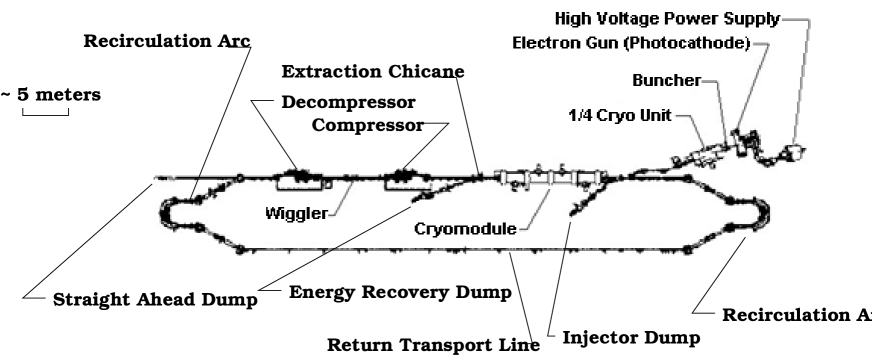
A generic ERL-driven FEL is pictured in Figure 1. The electron beam, assumed to be relativistic (so that $\beta\simeq 1$ and the momentum equals the energy), is injected in the ERL main linac with an energy of $\gamma_{o}$, and rms energy spread $\sigma_{\gamma_{o}}$. The main linac consists of an RF-accelerating section providing an energy gain amplitude $\gamma_{rf}$ and operating with a phase $\varphi_{rf}$ (the phases being referenced to the maximum acceleration phase). The undulator is located downstream from the linac, after the beam has been compressed in a magnetic bunch compressor. After participating in the FEL process, the beam is recirculated and re-injected into the accelerating section (on the decelerating phase $\pi-\varphi_{rf}$) via the so-called recirculator. The recirculator has several functions:

1. it bends the beam by a total angle of 360^∘,

2. it provides tuning of the transport path length (to re-inject the beam into the accelerating section with the proper phase),

3. it provides variable tuning of bunch time-energy chirp.

In the Ir-Demo, the decelerated beam is split off the main beam-line by a dipole and the beam is dumped.

The longitudinal dynamics is given by three requirements: (1) the beam incoming energy needs to be matched to the FEL resonance condition, (2) the beam must have a high peak current at the undulator location, and (3) the recirculator should be optimized to minimize the momentum spread after the deceleration so the spent beam is cleanly dumped.

II.1 Operation of the free-electron laser

Energy gain through the RF-accelerating section:

Downstream from the accelerating section an electron, of coordinate $s$ with respect to the bunch centroid, after the accelerating pass gains the energy:

$$\gamma_{U}(s)= \gamma_{o}(s)+\gamma_{rf}\cos(k_{rf}s+\varphi_{rf})\mbox{.}$$ (1)

where $k_{rf}$ stands for the RF-field wave vector ($k_{rf}\doteq 2\pi/\lambda_{rf}$, $\lambda_{rf}$ being the RF-wavelength). The average beam energy, $\langle{\gamma_{U}}\rangle$, at the undulator location, is: $\mbox{$\langle{\gamma_{U}}\rangle$}=\mbox{$\langle{\gamma_{o}}\rangle$}+\gamma_{rf}\cos\varphi_{rf}$

The FEL resonance condition:

Given the wavelength $\lambda$ at which the FEL must operate, the electron beam energy must fulfill the resonance condition:

$$~{}\gamma_{U}=\sqrt{\frac{\lambda_{u}}{2\lambda}(1+K^{2}/2)}$$ (2)

where $\lambda_{u}$ is the undulator period, and $K$ the undulator parameter.

The minimum bunch length condition:

Since the injector cannot directly provide the required high-peak current, it is necessary to compress the electron bunch by means of magnetic compression. We characterize the compressor by its first order momentum compaction, $R^{C}_{56}$, defined as the linear dependence of the path length though the compressor on the fractional momentum offset $\delta$. Under such a linear assumption, an electron of initial coordinate $(s_{i},\delta_{i})$ is mapped to the final longitudinal position as: $s_{f}\simeq s_{i}+R^{C}_{56}\delta_{i}$. If we assume there is no local momentum spread, the minimum bunch length ($s_{f}=0$) is achieved when the incoming longitudinal position-momentum correlation satisfies the relation:

$$\left[\frac{d\delta}{ds}\right]_{s=0}= -\frac{1}{R^{C}_{56}}\mbox{.}$$ (3)

In Eq. 3, we assume the fractional momentum offset is small enough that second order dependencies on this quantity are insignificant; i.e. we assume

$$|\delta|\ll\big{|}\frac{R^{C}_{56}}{T^{C}_{566}}\big{|}\mbox{,}$$ (4)

where $T^{C}_{566}$ denotes the second order dependence of the path length in the compressor on the fractional momentum offset. For an achromatic chicane, under the small bending angle approximation, we have raubenheimer-pac87 $T^{C}_{566}/R^{C}_{56}\simeq-3/2$.

Eqs. 1, 2 and 3 yield the following values for the required phase and amplitude of the accelerating RF-section:

$$\tan\varphi_{rf}= \frac{\lambda_{rf}}{2\pi R_{56}}\times\frac{\gamma_{U}}{\gamma_{U}-\gamma_{o}}\mbox{, and}$$ (5)

$$\gamma_{rf}=\frac{\gamma_{U}-\gamma_{o}}{\cos\varphi_{rf}}$$ . (6)

II.2 Recirculation

Longitudinal phase space after the FEL interaction:

After the electron bunch has contributed to the FEL process, an electron loses an energy of $\Delta\Gamma$ on average and the fractional momentum spread of the bunch is increased. The average energy downstream from the undulator is: $\mbox{$\langle{\gamma_{U+}}\rangle$}=\mbox{$\langle{\gamma_{U}}\rangle$}-\Delta\Gamma$ .

Longitudinal dynamics in the recirculator:

As mentioned previously, the recirculator provides a zeroth order optics knob: it allows one to tune the path length in such a way that the beam centroid is injected in the RF-section with the phase $\psi_{rf}=\pi-\varphi_{rf}$. In addition, the recirculator is used to manipulate the longitudinal phase space, because it provides $360^{\circ}$ bending and generates dispersion (to arbitrary order) which can be used to control the linear and quadratic (and higher order) dependence of path length on fractional momentum spread in the recirculator. Because the incoming momentum spread is large, depending on the geometric arrangement of the bending system, a relation as in Eq. 4 may not be satisfied, and hence higher order contributions to the longitudinal transfer map need to be included. It is necessary to expand the longitudinal map to the second order in $\delta$. Let ${\bf x}^{U+}=(x,x^{\prime};y,y^{\prime};s,\delta)^{U+}\doteq(x_{1},x_{2},x_{3},x_{4},x_{5},x_{6})^{U+}$ be the coordinates of the electron at the undulator exit and ${\bf x}^{R}$, those after the recirculation, i.e. at the linac entrance. Under the single-particle-dynamics approximation, the transport from the undulator exit to the linac entrance can be modeled by the longitudinal map ${\mathcal{Z}}$ that is generally Taylor-expanded:

$$x^{U+}_{k}\stackrel{{\scriptstyle\mathcal{Z}}}{{\rightarrow}}x^{R}_{k}=\sum_{i}\frac{\partial{\mathcal{Z}}_{k}}{\partial x^{U+}_{i}}x^{U+}_{i}+\frac{1}{2}\sum_{i}\sum_{j}\frac{\partial^{2}{\mathcal{Z}}_{k}}{\partial x^{U+}_{i}\partial x^{U+}_{j}}x^{U+}_{i}x^{U+}_{j}+{\cal O}\left(({\bf x}^{U+})^{3}\right)$$ (7)

which maps the $k$-th electron coordinate at the undulator exit to the entrance of the linac. We now define the first and second order Taylor coefficient (following the transport convention) as: $R_{ki}=(\partial{\mathcal{Z}}_{k})/(\partial x^{U+}_{i})$ and $T_{kij}=1/2\times(\partial^{2}{\mathcal{Z}}_{k})/(\partial x^{U+}_{i}\partial x^{U+}_{j})$. Using these definitions and only considering the $s$-coordinate we have:

$$~{}s^{U+}\stackrel{{\scriptstyle\mathcal{Z}}}{{\rightarrow}}s^{R}=(R_{55}+\sum_{j=1}^{4}T_{55j}x_{j}^{U+})s^{U+}+T_{555}(s^{U+})^{2}+(R_{56}+\sum_{j=1}^{5}T_{56j}x_{j}^{U+})\delta^{U+}+T_{566}(\delta^{U})^{2}+...\mbox{.}$$ (8)

Deceleration for energy recovery:

As the beam is decelerated in the RF-section, an electron of coordinate $s^{\prime}$ downstream of the recirculator will have the energy

$$\gamma_{D}(s^{\prime})=\gamma_{R}(s^{\prime})-\gamma_{rf}\cos(k_{rf}s^{\prime}+\psi_{rf})$$ , (9)

downstream of the RF-section. Here $\psi_{rf}=\pi-\phi_{rf}$ and $\gamma_{R}$ is the electron energy before deceleration (i.e. at the recirculator exit). From this latter equation the average energy takes the form: $\mbox{$\langle{\gamma_{D}}\rangle$}=\mbox{$\langle{\gamma_{o}}\rangle$}-\Delta\Gamma$. The quantity of interest after deceleration is the fractional momentum offset, $\delta^{D}(s^{\prime})=\gamma_{D}(s^{\prime})/\mbox{$\langle{\gamma_{D}}\rangle$}-1$;

$$~{}\delta^{D}(s^{\prime})=\frac{\gamma_{rf}\left[(k_{rf}s^{\prime})^{2}/2\cos(\psi_{rf})+k_{rf}s^{\prime}\sin(\psi_{rf})\right]}{\mbox{$\langle{\gamma_{U+}}\rangle$}-\gamma_{rf}\cos(\psi_{rf})}+\delta^{R}(s^{\prime})\frac{\mbox{$\langle{\gamma_{U+}}\rangle$}}{\mbox{$\langle{\gamma_{U+}}\rangle$}-\gamma_{rf}\cos(\psi_{rf})}$$ , (10)

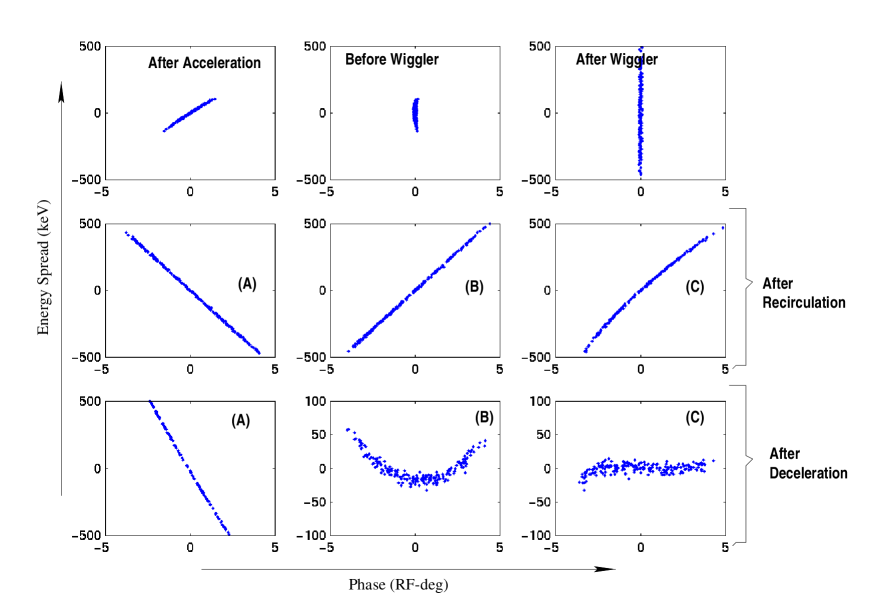
with $\delta^{R}(s^{\prime})$ being the fractional momentum offset upstream from the RF-section before the second pass. In Eq. 10, we have expanded the fractional momentum offset up to the second order in $s^{\prime}$ because the incoming bunch length, $\sigma_{s^{\prime}}$, does not a priori satisfies the condition $\sigma_{s^{\prime}}\ll 1/k_{rf}$. Eqs. 8 and 10 suggest a mechanism for counteracting the momentum spread generated during deceleration. The method consists of setting up the recirculator in a way to impart both a linear and quadratic a position-energy correlation, and allowing the bunch to decompress before the decelerating pass. Formally one wants to match the linear and quadratic dependence of $\delta^{R}$ to

$$\left[\frac{d\delta^{D}}{ds^{\prime}}\right]_{s^{\prime}=0}=-\frac{\mbox{$\langle{\gamma_{rf}}\rangle$}}{\mbox{$\langle{\gamma_{U+}}\rangle$}}k_{rf}\sin(\psi_{rf})\mbox{, and}\left[\frac{d^{2}\delta^{D}}{d^{2}s^{\prime}}\right]_{s^{\prime}=0}=-\frac{\mbox{$\langle{\gamma_{rf}}\rangle$}}{2\mbox{$\langle{\gamma_{U+}}\rangle$}}k^{2}_{rf}\cos(\psi_{rf})$$ (11)

where the latter equation insures the RF-induced curvature is canceled. The technique is illustrated in Figure 3. In this figure, the last row contains the longitudinal phase spaces downstream from the linac after deceleration for three different choices of recirculator optics. Plot (A) illustrates that the phase space slope should be properly chosen, as otherwise excessive energy spread results. Once the slope is properly chosen, plot (B) of this last row illustrates the importance of RF-induced curvature as an lower limit for momentum spread. In plot (C) we show how, using the recirculator to impart a quadratic dependence of the fractional momentum spread on the longitudinal position upstream from the linac, allows the compensation of RF-induced curvature which, in turn, greatly reduces the fractional momentum spread. In this latter case the fractional momentum spread is limited by a 3rd order aberration (as seen by the “S” shape of the phase space).

III Example of the Ir-Demo

In the Ir-Demo (see top view in Figure 2), the electron beam, is generated by a $350\,{\rm keV}$ photoemission electron gun engwall-pac97 , and accelerated piot_epac1998 to $\sim$10 MeV by two superconducting radio-frequency (SRF) CEBAF-type cavities (5-cell $\pi$-mode standing-wave cavities largely of the same design as those in the CEBAF accelerator arnps ) mounted as a pair in the so-called “quarter cryounit”. The beam is then injected into the main linac which is composed of one cryomodule, containing 8 CEBAF-type SRF cavities. The linac can provide a net energy gain of approximately $37\,{\rm MeV}$ (but is operated to provide 28 MeV energy gain for the results presented in this paper). The operating frequency of the RF-system is 1.497 GHz, so $\lambda_{rf}\simeq 0.20026$ m. This cryomodule is followed by two 4-bend achromatic chicanes that bypass the FEL resonator mirrors and provide longitudinal phase space manipulation. The first chicane, upstream from the undulator, serves as bunch compressor and the second chicane naturally decompresses the upright bunch. The undulator is located between the two chicanes. Soon after the downstream chicane the beam is recirculated, by the means of a recirculator with variable (linear and quadratic) momentum compaction and path length, back to the entrance of the cryomodule. The path length is chosen so the second pass bunches have the proper time of arrival: the electron bunches are on the decelerating phase of the radio-frequency wave. The electrons are decelerated down to 10 MeV and are separated from the 48 MeV beam and dumped in the “energy recovery dump” by the means of the “extraction chicane”.

A complete description of the driver-accelerator can be found in References douglas_pac97 ; douglas-linac2000 . In terms of the longitudinal beam dynamics, the first matching point is at the undulator location where a longitudinal waist (minimum bunch length) is required. Given the longitudinal phase space at the injector front-end, the SRF-linac settings must be tuned in amplitude and in phase for achieving the desired longitudinal phase space correlation, $\simeq d\delta/ds$, to match the momentum compaction $R_{56}^{C}\simeq-28.8$ cm of the first chicane according to Eq. 3. In the nominal operating conditions, the aforementioned requirements result in operating the linac $\varphi_{rf}=$$-10\,{\rm{}^{\circ}}$ off crest for an accelerating voltage of approximately $\gamma_{rf}m_{e}c^{2}=$$37\,{\rm MeV}$ to provide an FEL wavelength $\lambda\simeq$$5\,{\rm\mu m}$. Downstream from the undulator the beam-line consists of (1) a magnetic chicane similar to the one upstream but which now acts as a bunch decompressor, and (2) a recirculation loop. The recirculation loop incorporates two 180 ^∘ arcs linked by a straight line section, the “return transport line”, which consists of six FODO cells having a $90^{\circ}$ betatron phase advance per cell. The arcs are based on the MIT-Bates accelerator design flanz-nima85 ; they each provide a total bending angle of $180\,{\rm{}^{\circ}}$. They include four wedge-type dipoles, each bending the beam by an angle of about $\pm 28\,{\rm{}^{\circ}}$ alternatively, installed in pairs symmetrically around a $180\,{\rm{}^{\circ}}$ dipole. In addition to providing the desired bending, the arcs are also used to adjust the total beam path length of the recirculated beam. For such purposes, the arc is instrumented with a pair of horizontal steerers located upstream and downstream the 180 ^∘ dipole to vary the reference orbit path length inside the 180 ^∘ magnet. This provides a path length adjustment of the order of $\pm\lambda_{rf}/2$ off the nominal length ($\simeq 501.5\times\lambda_{rf}$).

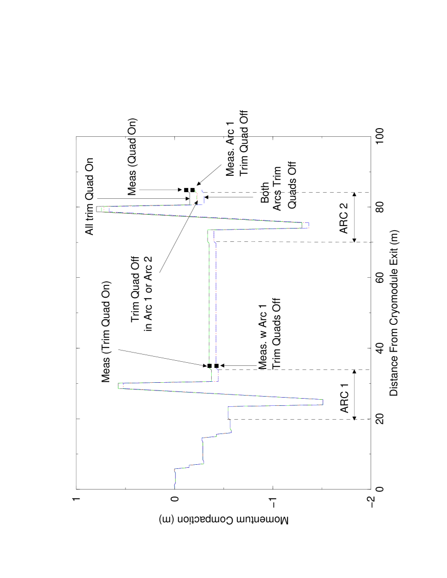
Two families of quadrupoles (the trim quadrupoles) and sextupoles are installed in the arc to provide both linear and quadratic energy dependent path length variation that are necessary in the “energy-compression” scheme needed to properly energy recover the beam douglas-tn98-025 . The quadrupoles act both on the linear and quadratic momentum compaction of the recirculator (these quantities are henceforth noted $R^{U+\rightarrow R}_{56}$ and $T^{U+\rightarrow R}_{566}$) while the sextupoles only impact the quadratic momentum compaction; the magnitude of the impact of these elements on the momentum compaction is illustrated in Figure 4. When the quadrupoles and sextupoles are unexcited, the arcs are operated in a non-isochronous mode ($R^{A}_{56}=13.1$ cm for a single 180^∘ arc). However under nominal operation, i.e. when the FEL is operating and the linac is in energy recovery mode, because of the need for energy compression, the sextupoles and quadrupoles of one family are excited to proper values in order to provide the required parameters. The momentum compaction of the recirculation loop is related to those of the individual components via:

$$R_{56}^{U+\rightarrow R}=R_{56}^{C}+R_{56}^{A1}+R_{56}^{A2}\mbox{,}$$ (12)

where the subscript $C$, $A1$ and $A2$ indicate the quantity corresponds respectively to the “decompressor” chicane, the first and second arc. Similar relations yield for the second order momentum compaction.

IV experiment in the Ir-Demo

IV.1 Measurement of the initial conditions at the undulator

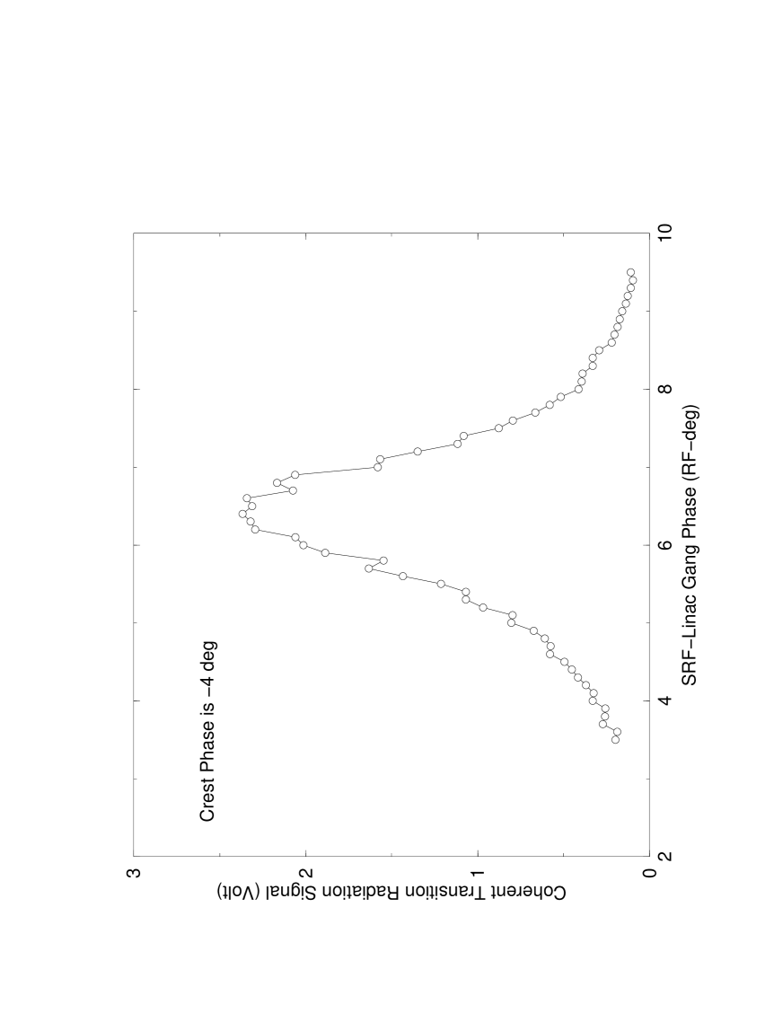
Experimentally, the accelerator module amplitude is set up accordingly to numerical simulation, then the phase is tuned to obtain the minimum bunch length at the undulator (i.e. the highest peak current). The bunch length is monitored krafft-epac1998 by detecting the coherent transition radiation (CTR) emitted in the backward direction as the electron bunch crosses an aluminum foil adjacent to the undulator. The power density radiated by a bunch of $N$ electrons is

$$[\frac{dP}{d\omega d\Omega}]_{N}=[\frac{dP}{d\omega d\Omega}]_{1}\times(N+N(N-1)|\int^{+\infty}_{-\infty}dtS(t)\exp-i\omega t|^{2})$$ , (13)

where $[\frac{dP}{d\omega d\Omega}]_{1}$ is the single electron power density. Thus since the Fourier transform of a bunch with characteristic length $\sigma_{s}$ extends to frequency $\omega\sim c/\sigma_{s}$, detecting the CTR at frequencies close to this frequency provides indirect information on the bunch length. An example of such a measurement is presented in Figure 5.

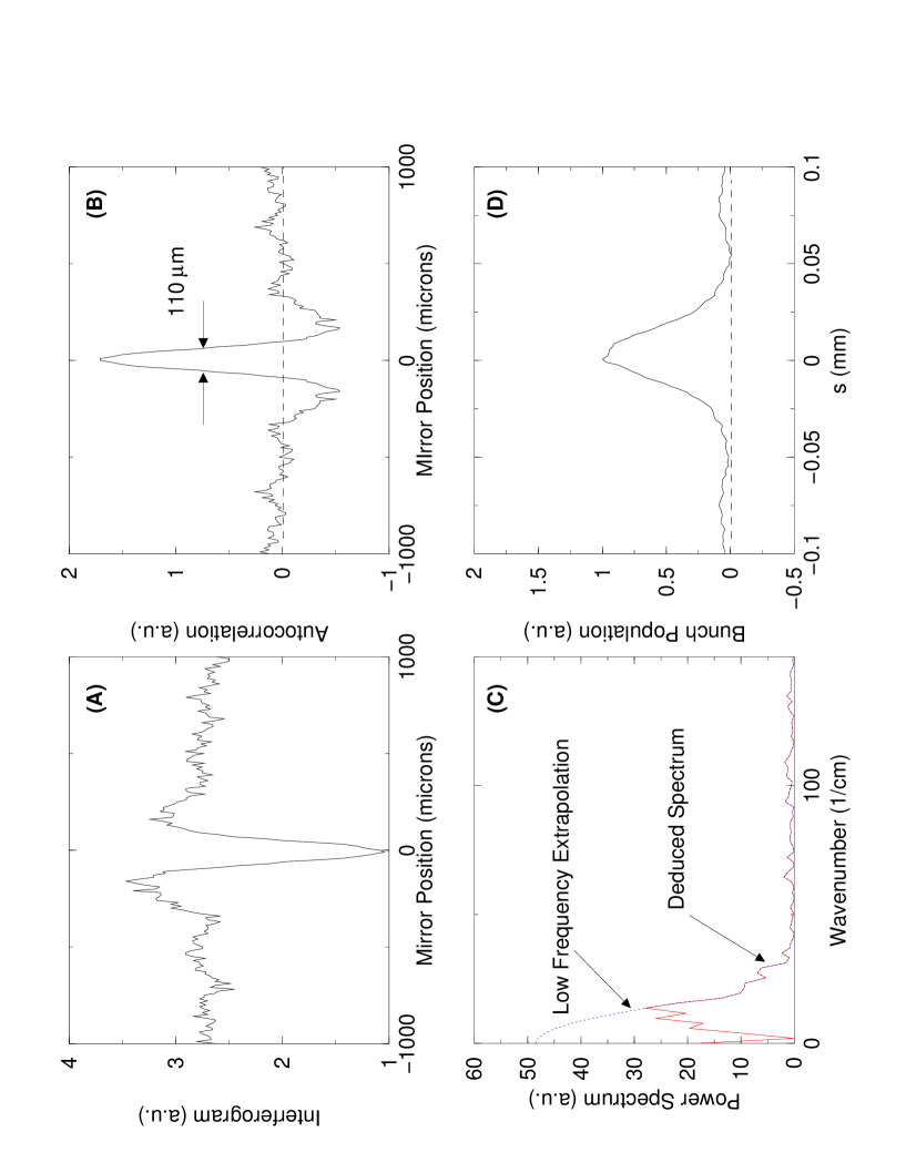
Once the phase is properly tuned, the bunch length is measured by performing Michelson interferometry happek-prl ; piot-tn of the CTR signal, since the radiation pulse emitted by the electron bunch mirrors the electron distribution. From the measured interferogram, one can deduce the autocorrelation function and (in virtue of the Wiener Kintchine theorem) the power spectrum of the CTR. A logarithmic Hilbert-transform burge-Lond76 ; lai-pre95 of the latter power spectrum allows one to reconstruct the electron longitudinal charge density. A typical measurement of an interferogram along with the subsequent calculations is shown in Figure 6. Routinely, the bunch length achieved in the Ir-Demo FEL is approximately $100$ $\mu$m (rms) for a bunch charge of 60 pC.

The fractional momentum spread of the beam is deduced from a profile measured at the high dispersion point of the decompressor chicane; the three quadrupoles upstream from the chicane are used to insure the betatron contribution to the beam profile is insignificant. In Figure 7 we compare the fractional momentum profiles with and without operating the FEL (the FEL process can be turned on/off by tuning/detuning the length of the optical resonator). The typical rms fractional momentum spread before the FEL interaction is about 0.4%, which grows to to 1.2% downstream from the FEL when the laser operates.

At the undulator location, the bunch length has been minimized, the longitudinal phase space is thus expected to be up-right; i.e. no position-energy correlation exists.

IV.2 Experimental setup to measure longitudinal transfer maps

The measurements of the longitudinal transfer map ${\cal Z}$ is very difficult. Instead, we perform a perturbative measurement which provides information on the Taylor expansion of the map. The technique consists of perturbing the initial conditions at a given location $i$ (initial RF-phase, $\phi^{i}=2\pi s^{i}/\lambda_{rf}$, or initial energy $\delta^{i}$) and measuring the relative time-of-flight (TOF) to a downstream position $f$ (the time-of-flight is also measured in RF-phase units). The two aforementioned excitations allow the perturbative measurement of the $\partial s^{f}/\partial s^{i}$ or $\partial s^{f}/\partial\delta^{i}$ expansions of the map which gives (see Eq. 8):

$$~{}\frac{\partial s^{f}}{\partial s^{i}}=R_{55}^{f\rightarrow i}+\sum_{j}T_{55j}^{f\rightarrow i}x_{j}+2T_{555}^{f\rightarrow i}s^{i}\mbox{ and,}$$ (14)

$$~{}\frac{\partial s^{f}}{\partial\delta^{i}}=R_{56}^{f\rightarrow i}+\sum_{j}T_{56j}^{f\rightarrow i}x_{j}+2T_{566}^{f\rightarrow i}\delta^{i}\mbox{.}$$ (15)

Henceforth we will term $\partial s^{f}/\partial s^{i}$ and $\partial s^{f}/\partial\delta^{i}$ respectively as “compression efficiency” and “momentum compaction” maps, and we will instead work in RF-phase unit: $\partial s^{f}/\partial s^{i}\rightarrow\partial\phi^{f}/\partial\phi^{i}$ and $\partial s^{f}/\partial\delta^{i}\rightarrow\partial\phi^{f}/\partial\delta^{i}$. In essence, the measurement of the compression efficiency or momentum compaction maps reduces to a relative TOF variation measurement.

Measurement of TOF is performed by detecting the phase of a signal produced by the TM₀₁₀ waves excited as the electron bunches traverse a resonant 1.497 GHz stainless steel cavity krafft_aip_95 ; piot_epac2000; hardy-pac97 . The principle of the TOF measurement is to measure the phase of the beam induced voltage since it has constant phase with respect to the electron bunches. The phase of the rf signal coming from the cavity is mixed with the reference signal, which may be phase shifted by means of a programmable phase shifter. The mixer output, after removal of high frequency component with a low pass filter, is calibrated by performing a procedure that consists of varying the phase shifter to find the output maxima from the mixer. Once the measurement is calibrated, the phase shifter phase is set so that for the nominal conditions of the machine the cavity is operated at zero-crossing of the mixer. Thus a change in TOF give rise to a linear change in the mixer output.

The change in the TOF induced by perturbing the beam initial phase or energy condition upstream can provide $\partial\phi^{f}/\partial\phi^{i}$ or $\partial\phi^{f}/\partial\delta^{i}$ respectively. In the Ir-Demo the former kind of measurement is performed by varying the phase of the photo-cathode drive laser (with respect to the RF-master oscillator) whereas the latter type of measurement is done by modulating the gradient of the last SRF-cavity of the cryomodule. In the accelerator three pickup cavities have been installed. Their locations are downstream of: (1) the crymomdule (C1), the (2) first 180 ^∘ (C2) and (3) second 180 ^∘ arc (C3). To expedite the measurements, the quantity varied (i.e. laser phase for $\partial\phi^{f}/\partial\phi^{i}$ transfer map and cavity gradient for $\partial\phi^{f}/\partial\delta^{i}$ transfer map), is varied at 70 Hz during the acquisition of measurement data.

IV.3 Numerical model for calculation of longitudinal transfer map

The measurement of the compression efficiency map provides important information on the performance of the bunching process and can give some insights on the bunch length. Because the map is measured between the photocathode and the pickup cavities, it cannot be simulated using standard single particle dynamics codes, but needs to be computed using a particle tracking code, e.g. parmela parmela_refer , which includes non relativistic effects such as phase slippage effects in accelerating cavities. The technique we have used to compare the measurements with numerical simulations is as follows: we use parmela to generate uniform macroparticles distribution over a given extent in RF-phase (or time) at the photocathode surface. The corresponding phase of emission $\phi_{k}^{i}$ of the $k$-th macroparticle at the photocathode surface is recorded and the macroparticles populating this uniform distribution are tracked along the beam-line. For the tracking the space charge subroutine is not activated, and each macroparticle is assumed to be the bunch centroid of bunches emitted at different drive-laser phase, we then compute the phase of arrival $\phi_{k}^{f}$ at the desired pickup cavities. The couple ($\{\phi_{k}^{i}$, $\phi_{k}^{f}\}_{k=1,...,N}$) directly gives the phase-phase transfer map which can be compared to the experimental data.

In order to generate energy-phase transfer maps, we use the arbitrarily high order code TLie tlie-refer based on a symplectic integrator: the energy offsets achieved when modulating the gradient of the last cryomodule cavity are directly used by the code to calculate the TOF up to the desired the pickup cavity. The couple ($\{\delta_{k}^{i}$, $\phi_{k}^{f}\}_{k=1,...,N}$) provides the energy-phase correlation and again can be compared with the data.

IV.4 Path length adjustment

In passing we note that one of the installed detectors can also be used to precisely setup the path length of the recirculator; in such a case the detector C1 is used. The beam is first dumped in the “straight ahead dump” (see Fig. 2) and the phase of the reference signal used for C1 is shifted so that the signal at the mixer output is maximized. The beam is then recirculated and the path length is varied using the dedicated horizontal steerers located at both entrance and exit of the two 180^∘ bends. The path length is optimized when the signal measured at C1 is zeroed: this corresponds to the case when the beam induced voltage generated by the first pass and recirculated beams exactly cancel.

IV.5 Experiments and simulations

The compression efficiency and momentum compaction transfer map measurement have been extensively used during the commissioning of the Ir-Demo, to verify our model, but also in routine operation, to insure the accelerator, and especially the recirculator loop, is properly set up.

IV.5.1 Compression efficiency

In Figure 8, we compare a typical measurements of the $\partial\phi^{f}/\partial\phi^{i}$ maps at the three different detectors (C1, C2, and C3) with the maps generated via simulations. We generally observe a good agreement with between the measurement and the expectations. The slight disagreement, e.g. as the one observed at detector C3, is attributed to mis-steering in the arc 2 which makes larger the contribution of the $T_{55j}$ terms (with $j=1,...,4$) in Eq. 14. The second arc transport is more vulnerable to such misalignments since the bunch length is larger compared to arc 1.

More quantitative information can be obtained by performing a nonlinear fit of the transfer map presented in the Figure. This can give some insight on the linear $R_{55}$ and quadratic, $T_{555}$ compression efficiency coefficients between the photocathode and the pickup cavities: the results are presented in Table 1.

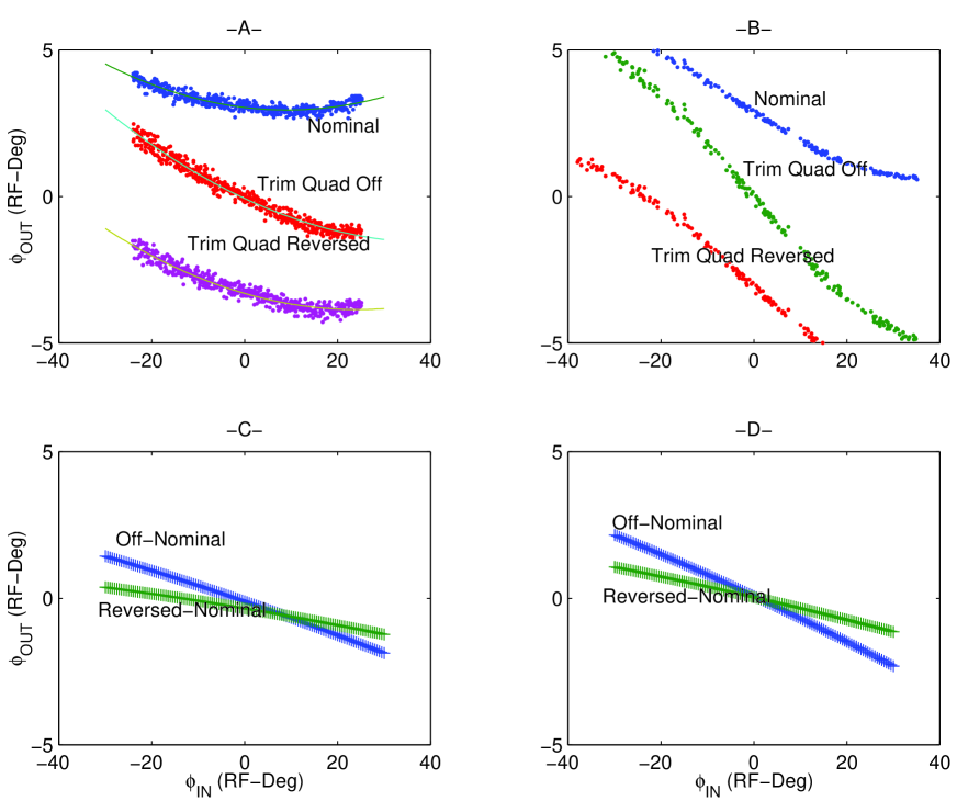
The compression efficiency map measurement was also used as a trouble shooting tool. In Figure 11 we present a series of measurement we performed using the detector C2: the compression efficiency was measured for three settings of one of the quadrupole pairs of arc 1: (a) the quadrupoles are excited to their nominal values, (b) they are turned off, and (c) they are powered to a value opposite to case (a). The comparison of the measured transfer map with the simulated one shows some disagreement (at that time we could not accurately know precisely the machine settings of the upstream beam-line, e.g., in the injector). However, if one compares the difference measurement (i.e. calculated as (b)-(a) and (b)-(c)) with the corresponding difference simulations, the agreement becomes very good. Such an example illustrates how a measurement of transfer maps for various perturbations of the lattice (here using quadrupole pairs) can be used to verify that the different lattice elements that compose the beam-line perform as expected. This method was in fact used to diagnose a reinjection phase error during commissioning douglas-sum .

IV.5.2 Momentum compaction:

The momentum compaction transfer map was measured by modulating the gradient of the last cryomodule cavity by $\pm 1$%.

The linear expansion of the transfer map, $R_{56}$, was measured at both C2 and C3. In Figure 10, we compare the expected evolution of the linear momentum compaction for different excitations of the “trim quadrupoles” with the measurement obtained at C2 and C3: the agreement is excellent. A more quantitative measurement was performed using C2, the momentum compaction from the cryomodule exit up to C2 was measured as a function of the trim quadrupole settings, the comparison of such a measurement with the expected values obtained with the second order optics code dimad dimad-refer , again the good agreement confirms the usefulness of time-of-flight diagnostics for setting up the recirculation.

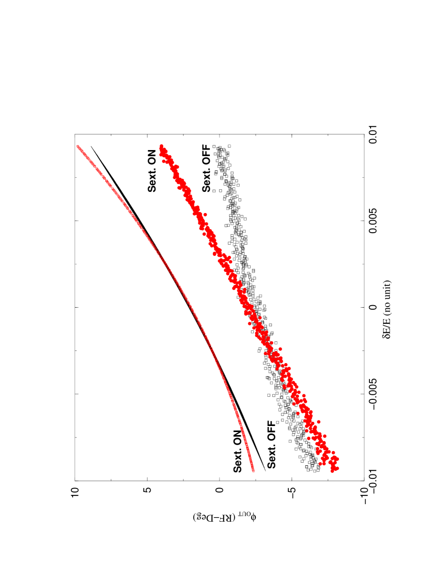
The sensitivity of the momentum compaction map to second order changes in the optics, e.g. imparted by the sextupoles, was also investigated. Figure 12 depicts the impact of exciting one of the sextupole pairs of arc 2 on the map measured by the detector C3. The effect observed in simulations and measurements is the same: in both cases exciting the sextupole impress a positive curvature on the map – though the agreement is not absolute. This can again be explained by the sensitivity of the nonlinear terms to mis-steering via the second order chromatic functions $T_{56i}$ (with $i=1,...,4$). Especially when the FEL is operating, the aforementioned effect is enhanced because of the large FEL-induced fractional momentum spread.

IV.5.3 Other experimental evidence of energy compression:

The primary evidence of the good performance of the energy compression scheme was our ability to recover 5 mA average current beam while lasing at high gain with an average output power of 2.1 kW without any beam losses. The Ir-Demo is equipped with a high sensitivity protection system that can detect localized losses of beam as low as 1 $\mu$A beamlosses .

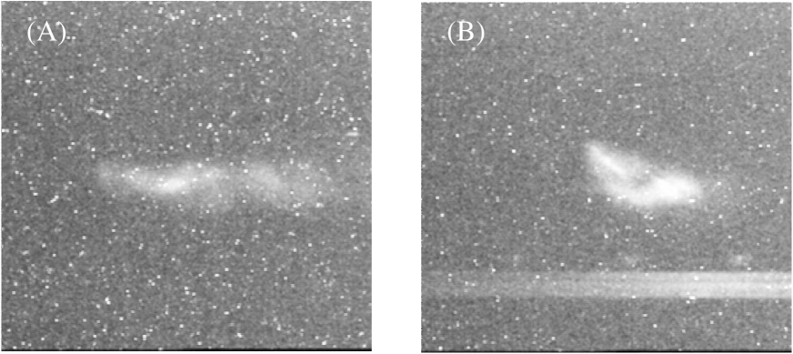
Another validation of the method is to observe the beam transverse density on the energy recovery dump aluminum window. Such a measurement was performed by detecting the backward optical transition radiation (OTR) emitted at the interface vacuum/aluminum of the window. The OTR images are detected with a charge couple device (CCD) camera and digitized for analysis. At the window the dispersion (horizontal) is $\eta\simeq 1$ m. The results of our observations are presented in Figure 13: when the longitudinal compression is properly tuned the beam is tightly focused whereas by slightly mis-setting one pair of sextupoles (which does not affect $-$ to first order $-$ the lattice functions), the beam horizontal size starts to blow-up, indicating relatively poor energy spread.

V Conclusion

We have successfully characterized the energy compression scheme to recover the “spent” electron beam after the FEL-process in the IR-demo. Such techniques are well adapted for energy-recovering an electron beam in a moderate power FEL. For very high power FELs anticipated in the future, higher order corrections and/or the use of a dedicated “accelerating” section to impart the required position energy correlation might be needed. As an example the forthcoming upgrade of the Ir-Demo to 10 kW requires the use of octupoles douglas-10kW-linac2000 .

The techniques we have developed for characterizing the longitudinal lattice maps have proven to be a valuable tool both during the commissioning of the Ir-Demo FEL but also for its day-to-day operation: under the nominal setup of the recirculator the map pattern is well defined and changes of this pattern indicate one of the component in the recirculator or RF-system is not properly set. However there is room for improvement: we have shown that in some cases, e.g. due to mis-steering of the beam in the arcs, the extraction of quantitative information from the transfer map may turn out to be difficult. A way of improving this situation is to measure the transfer map for different steering conditions. By doing such a “two dimensional difference orbit” measurement, one could get information on the coupling terms (e.g. $T_{55j}$ or $T_{56j}$) and thus correct accordingly the measurement to be less sensitive to misalignment.

VI Acknowledgments

This work was sponsored by US-DOE grant number DE-AC05-84ER40150, the Office of Naval Research, the Commonwealth of Virginia and the Laser Processing Consortium.

Detector	Linear Coeff.	Quadratic Coeff.
Experiment
C1	0.12	8$\times 10^{-4}$
C2	-0.08	16$\times 10^{-4}$
C3	0.09	6$\times 10^{-4}$
Simulation
C1	0.11	7$\times 10^{-4}$
C2	-0.08	3$\times 10^{-4}$
C3	0.03	4$\times 10^{-4}$

Table 1: Measured and simulated linear and quadratic expansions of the compression efficiency map at the three detector location (C1, C2, and C3).

Figure 1: Generic configuration for an energy recovering driven free-electron laser.

Figure 2: Overview of the Ir-Demo free-electron laser of Jefferson Lab.

Figure 3: Energy compression scheme: The first row (from left to right) presents the longitudinal phase space at the linac exit, after the compression chicane, and just after the wiggler interaction has taken place; the second row show longitudinal phase space at the entrance of the linac just prior to deceleration for three different choice of $R_{56}$ and $T_{566}$ ( for (A) -0.2 and 0. m, for (B) 0.2 and 0 m and for (C) 0.2 and 3.0 m). The result for the three cases after deceleration are shown in the third row.

Figure 4: First ($R_{56}$) and second ($T_{566}$) order momentum compaction evolution, for one arc of the recirculator, versus the settings of the trim quadupoles and sextupoles.

Figure 5: CTR signal versus SRF-linac phase. The maximum CTR signal coincides with the shortest achieved bunch length. For the corresponding phase, the longitudinal phase space is up-right.

Figure 6: Example of bunch length measurement. (A) raw data obtained from the Michelson polarizing interferometer, (B) deduced autocorrelation from the interferogram, (C) power spectrum obtained by Fourier-transforming the autocorrelation, (D) charge density longitudinal distribution obtained by applying the Kroenig-Kramer relations on the power spectrum to recover the (missing) phase information.

Figure 7: Impact of the FEL process on the beam fractional momentum profile. The energy profiles are measured in the ”decompressor” symmetry point.

Figure 8: Comparison of the phase-phase beam transfer function between the photocathode surface and the three different pickup cavities (pickup C1, C2, and C3) (bottom row) with the one simulated using parmela (top row).

Figure 9: Comparison between the expected and measured linear momentum compaction, $R_{56}$, for the whole recirculation transport, versus different settings for one of the trim quadrupole pairs in one of the 180-deg arc.

Figure 10: Evolution of the linear momentum compaction along the beam-line, from the linac exit to the linac entrance.

Figure 11: Example of a difference compression efficiency transfer map measurement at the detector C2. The map is measured (A) and simulated (B) for three excitations of one pairs of trim quadrupole in the arc 1 (quadrupoles set up to their nominal values, turned off, and set up to a value opposite to their nominal value). Though the simulated and measured maps differ, the measured (C) and (D) simulated difference maps results are in better agreement.

Figure 12: Effect of the sextupole of arc 2 on the momentum compaction transfer map measured with the detector C3.

Figure 13: Beam density on the energy recovery dump aluminum window observed via optical transition radiation. The sextupoles in the arc 2 are turned off (A), and excited to their nominal value (B).

References

- (1) Tigner M., Nuovo Cimento 37, 1228-1231 (1965)
- (2) Douglas D.R., Proc. Part. Acc. Conf. 1997 IEEE cat.# 97CH36167, 1351-1355 (1997)
- (3) Neil G. R., et al., Phys. Rev. Lett., vol. 84, num. 4, 662-665 (2000)
- (4) Merminga L., et al. Nucl. Instr. Meth. A 429, 58-64 (1999)
- (5) Douglas D.R., for the Ir-Demo FEL project team, Proc. of LINAC conf. 2000, SLAC report R-561, 716-720 (2001)
- (6) Raubenheimer T.O., et al., Proc. Part. Acc. conf. 1993, IEEE cat.# 93CH3279-7, 635-637 (1993)
- (7) Engwall D., et al. Ibid douglas_pac97 , 2693-2695
- (8) Piot P., et al., Proc. Eur. Part. Acc. conf. 1998, 1447-1449 (Institute of Physics London 1998)
- (9) Leemann C. W., Douglas D. R., and Krafft G. A., Annual Rev. of Nucl. and Part. Sci. 51, 413-450 (2001)
- (10) Flanz J.B. and Sargent C.P., Nucl. Instr. Meth. A 241, 325-333 (1985)
- (11) Douglas D.R., “Lattice issues affecting longitudinal phase space management during energy recovery. Or, Why do we need sextupoles?”, report TN-98-025, Jefferson Lab, Newport News VA, USA (1998)
- (12) Krafft G.A., et al., Ibid piot_epac1998 , 1580-1582
- (13) Happek U., et al., Phys. Rev. Lett., vol. 67, num. 4, 2962-2967 (1991)
- (14) Piot P., et al., “Bunch length measurement using coherent transition radiation in the FEL”, report TN-99-003, Jefferson Lab, Newport News VA, USA (1999)
- (15) Burge R.E., et al, Proc. Roy. Soc. Lond. A350, 191-212 (1976)
- (16) Lai R., and Sievers A.J., Phys. Rev., E52, num. 2, 4576-4579 (1995)
- (17) Krafft G.A., AIP conf. proc. 367, 46-55 (1995)
- (18) Piot P., Douglas D.R., Krafft G.A., Ibid piot_epac1998 , 1543-1545
- (19) Hardy D., et al. Ibid douglas_pac97 , 2265-2267
- (20) Liu H., private communication, code initialy written by K. Crandall and L Young
- (21) van Zeijt J., TLie code, private communication
- (22) Sevranckx R.V., Brown K.L, Schachinger L., and Douglas D., SLAC report 285, (1985)
- (23) Douglas D.R., “Beam Transport Issues in the Winter/Spring 1999 FEL Run”, report TN-99-008, Jefferson Lab, Newport News, VA, USA (1999)
- (24) Jordan K., private communication
- (25) Douglas D.R., et al. “Driver Accelerator Design for the 10 kW Upgrade of the Jefferson Lab IR FEL”, Ibid douglas-linac2000