The driven pendulum at arbitrary drive angles

Abstract

We discuss the equation of motion of the driven pendulum and generalize it to arbitrary driving angle. The pendulum will oscillate about a stable angle other than straight down if the drive amplitude and frequency are large enough for a given drive angle. The emphasis is on the parameters associated with a simply made demonstration apparatus.

I Introduction

The general theory of the driven inverted pendulum with the drive angle restricted to 180^∘ is given in Ref. Landau, and has been discussed in Refs. FMP, ; DCM, ; EIB, ; the latter reference includes a good introduction to the physical system and further citations. In the following, the behavior of the harmonically driven pendulum will be described for any drive angle from the vertical.

An inverted pendulum demonstrationJones that is designed to be clamped to a table top becomes more interesting when hand held. We will examine the stability of this system as a function of the angular frequency, the drive amplitude, and the drive angle from the vertical. This type of demonstration is best used in a junior level classical mechanics course when introducing Lagrange’s equations to find the equations of motion. Examples of driving the support of a simple pendulum harmonically can be introduced, but only to set up the equation of motion.Marion ; Symon The same apparatus can be used in an advanced graduate classical mechanics course where the harmonically driven pendulum is used as an example of Lagrange’s equations and as a source of problems.Landau

While holding the saw in my hand,m17q with the power still on, I lowered the saw and observed the peculiar behavior of the pendulum as it sometimes found new stable angles of oscillation as the drive angle changed. Changing the driving angle in the plane of the pendulum’s motion introduces the new and interesting problem that I address in this paper.

II Equation of Motion of the Pendulum Driven at Any Angle

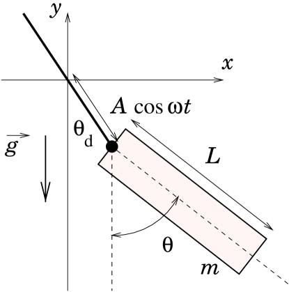
The dynamics of a driven inverted pendulum near $\theta=180^{\circ}$ are described in Refs. Landau, ; FMP, ; DCM, ; EIB, . We now generalize the problem to arbitrary driving angles. The geometry of the problem is illustrated in Fig. 1. A thin uniform rod of length $L$ is driven at one end (pivot) with amplitude $A$, angular frequency $\omega$, at an angle of $\theta_{d}$ from the downward vertical. The angle of the thin rod is measured by the generalized coordinate $\theta$ which also is measured from the vertical downward. (We also could have used a simple pendulum consisting of a mass $m$ at the end of a light rod of length $\ell$, or a general pendulum with moment of inertia $I$ and center of mass at a distance $z$ from the pivot. The rod pendulum geometry chosen here corresponds to a simple lecture apparatus.Jones ; m17q A different pendulum geometry can be easily substituted into the equations of motion below.)

The angle of the rod $\theta$ could be measured from the driving direction, $\theta_{d}$. However, for only two values of $\theta_{d}$ (0 and $\pi$) will the equilibrium angle of the pendulum be $\theta_{d}$. For any value of $\theta_{d}$, there is a stable point for small $\omega$ and $A$ at $\theta=0$. So we choose to measure the pendulum angle $\theta$ from the downward vertical.

The kinetic energy and potential energy of the rod can be written in terms of the generalized coordinate $\theta$. The energies are separated into the motion of the center of mass plus the rotation about the center of mass. We first express the Cartesian coordinates and velocities of the center of mass in terms of $\theta$.

$$x_{\text{cm}} = +{L\over 2}\sin\theta+A\sin\theta_{d}\cos\omega t$$ (1a)

$$y_{\text{cm}} = -{L\over 2}\cos\theta-A\cos\theta_{d}\cos\omega t$$ (1b)

$$\dot{x}_{\text{cm}} = +{L\over 2}\dot{\theta}\cos\theta-A\omega\sin\theta_{d}\sin\omega t$$ (1c)

$$\dot{y}_{\text{cm}} = +{L\over 2}\dot{\theta}\sin\theta+A\omega\cos\theta_{d}\sin\omega t.$$ (1d)

We can express the kinetic energy and potential energy in terms of the generalized coordinate $\theta$.

$$T={1\over 2}m(\dot{x}_{\text{cm}}^{2}+\dot{y}_{\text{cm}}^{2})+{1\over 2}I_{\text{cm}}\dot{\theta}^{2}.$$ (2)

If we use the Cartesian coordinates and velocities from Eq. (1), we obtain

$$T={1\over 2}\big{[}{{mL^{2}}\over{3}}\dot{\theta}^{2}+mLA\omega\dot{\theta}(\sin\theta\cos\theta_{d}-\cos\theta\sin\theta_{d})\sin\omega t+mA^{2}\omega^{2}\sin^{2}\omega t\big{]}.$$ (3)

The first term on the right-side of Eq. (3) corresponds to the rotation about the moving support at the end of the pendulum with a moment of inertia of $mL^{2}/3$ about that end.

The potential energy depends only on $y_{\text{cm}}$, and from Eq. (1) we have

$$V=mgy_{\text{cm}}=-{{mgL}\over 2}\cos\theta-mgA\cos\theta_{d}\cos\omega t.$$ (4)

The Lagrangian is ${\cal L}=T-V$, and using Eqs. (3) and (4), we have

$${\cal L} = {1\over 2}\big{[}{{mL^{2}}\over{3}}\dot{\theta}^{2}+mLA\omega\dot{\theta}\sin\big{(}\theta-\theta_{d}\big{)}\sin\omega t+mA^{2}\omega^{2}\sin^{2}\omega t\big{]}$$ (5)

$${}+mg\big{(}{L\over 2}\cos\theta+A\cos\theta_{d}\cos\omega t\big{)}.$$

The equation of motion is found from Lagrange’s equation for the single generalized coordinate $\theta$:

$${d\over{dt}}\big{(}{{\partial{\cal L}}\over{\partial\dot{\theta}}}\big{)}-{{\partial{\cal L}}\over{\partial\theta}}=0.$$ (6)

If we evaluate the derivatives of the Lagrangian from Eq. (5), we obtain the equation of motion for a pendulum driven at any angle:

$$\ddot{\theta}+{{3A\omega^{2}}\over{2L}}\sin(\theta-\theta_{d})\cos\omega t+{{3g}\over{2L}}\sin\theta=0.$$ (7)

Note that if $\theta_{d}=180^{\circ}$, we obtain the usual driven inverted pendulum.Landau ; FMP ; DCM ; EIB This special case is revisited briefly in Sec. IV.2 and in the Appendix.

III Effective potential

We now introduce an effective potential to help us understand the physical origin of the stability of the inverted pendulum and to parameterize the condition for stability at any driving angle.

Landau and LifshitzLandau separated the motion of the horizontally or vertically driven pendulum into two parts: a fast component $\xi(t)$ at the drive angular frequency $\omega$, and a slow component $\phi(t)$ that describes the slower overall swinging of the driven pendulum:

$$\theta(t)=\phi(t)+\xi(t)$$ (8)

The angle $\phi$ is defined as zero downward as is $\theta$, and $\xi$ is the difference between $\theta$ and $\phi$. In what follows we assume that the average of $\xi(t)$ (denoted as $\overline{\xi}$) is zero, and that $\xi(t)$ is small.

The equation of motion for a pendulum driven at any angle, Eq. (7), can be rearranged, in the form

$$\ddot{\theta}=-{{3g}\over{2L}}\sin\theta-{{3A\omega^{2}}\over{2L}}\sin(\theta-\theta_{d})\cos\omega t=F(\theta)+f(\theta,t).$$ (9)

We have separated the angular acceleration into a time dependent driving term $f(\theta,t)$ oscillating at the driving angular frequency $\omega$, and a time independent part $F(\theta)$ corresponding to the effect of gravity. Equation (9) can be rewritten in an expansion in $\xi$ for small values of $\xi(t)$:

$$\ddot{\phi}+\ddot{\xi}\simeq F(\phi)+{{dF}\over{d\theta}}(\phi)\xi+f(\phi,t)+{{df}\over{d\theta}}(\phi,t)\xi.$$ (10)

We keep only the largest rapidly varying terms on each side of Eq. (10) and write

$$\ddot{\xi}\simeq f(\phi,t)=-{{3A\omega^{2}}\over{2L}}\sin(\phi-\theta_{d})\cos\omega t.$$ (11)

Note that $\ddot{\xi}$ is $\omega^{2}$ larger than $\xi(t)$, so the terms in $\xi$ may safely be ignored. Also both $\ddot{\phi}$ on the left and $F(\theta)$ on the right do not oscillate at the driving angular frequency $\omega$.

Equation (11) may be integrated twice, taking the slow motion $\phi$ to be constant on the time scale $1/\omega$:

$$\xi(t)\simeq{{3A}\over{2L}}\sin(\phi-\theta_{d})\cos\omega t.$$ (12)

By averaging Eq. (9) over the fast component of the motion at angular frequency $\omega$, we obtain the equation of motion for the slow swinging of the pendulum:

$$\ddot{\phi}+\overline{\ddot{\xi}}\simeq F(\phi)+{{dF(\phi)}\over{d\theta}}\overline{\xi}+\overline{f(\phi,t)}+\overline{{{df(\phi,t)}\over{d\theta}}\xi}.$$ (13)

The rapidly oscillating terms $\ddot{\xi}$, $\xi$, and $f(\phi,t)$ average to zero, and we have

$$\ddot{\phi}\simeq F(\phi)+\overline{{{df}\over{d\theta}}(\phi,t)\xi}.$$ (14)

We then substitute for $F(\phi)$ and $df/dt$ from Eq. (9) and for $\xi(t)$ from Eq. (12). Only the $\cos\omega t$ terms vary rapidly, and so can be averaged on the longer time scale of the change of $\phi$. If we use $\overline{\cos^{2}\omega t}={1\over 2}$, we obtain the equation of motion for the angle $\phi$:

$$\ddot{\phi}\simeq-{{3g}\over{2L}}\sin\phi-{{9A^{2}\omega^{2}}\over{8L^{2}}}\cos(\phi-\theta_{d})\sin(\phi-\theta_{d}).$$ (15)

Equation (15) describes the slow swinging motion of the driven pendulum. If we use a simple trigonometric identity, we obtain another useful form of the equation of motion:

$$\ddot{\phi}\simeq-{{3g}\over{2L}}\sin\phi-{{9A^{2}\omega^{2}}\over{16L^{2}}}\sin[2(\phi-\theta_{d})].$$ (16)

The effective torque is the acceleration $\ddot{\phi}$ about one end of the rod multiplied by the moment of inertia about the end of the rod:

$$\tau_{\text{eff}}(\phi)={{mL^{2}}\over 3}\ddot{\phi}\simeq-{{mgL}\over{2}}\big{(}\sin\phi+{{3A^{2}\omega^{2}}\over{8gL}}\sin[2(\phi-\theta_{d})]\big{)}.$$ (17)

This torque can be derived from an effective potential energy, $V_{\text{eff}}(\phi)$, where $\tau_{\text{eff}}(\phi)=-dV_{\text{eff}}/d\phi$.

$$V_{\text{eff}}(\phi)=-{{mgL}\over{2}}\big{(}\cos\phi+{{3A^{2}\omega^{2}}\over{16gL}}\cos[2(\phi-\theta_{d})]\big{)}.$$ (18)

We define the dimensionless critical parameter, $R$, and the critical angular frequency, $\omega_{c}$:

$$R = {{3A^{2}\omega^{2}}\over{4gL}}={{\omega^{2}}\over{\omega_{c}^{2}}}$$ (19a)

$$\omega_{c} = \sqrt{{{4gL}\over{3A^{2}}}},$$ (19b)

and rewrite the effective potential from Eq. (18):

$$V_{\text{eff}}(\phi)=-{{mgL}\over{2}}\big{(}\cos\phi+{R\over 4}\cos[2(\phi-\theta_{d})]\big{)}.$$ (20)

The first term on the right side of Eq. (20) is simply the effect of gravity acting on the center of mass of the pendulum. The second term comes from the dynamics of the forced motion, and represents the average kinetic energy of the rapidly driven oscillation of the pendulum about its center of mass. As the pendulum deviates from the drive angle $\theta_{d}$, the angular kinetic energy of the pendulum about its center of mass increases.

If treated as an effective potential energy, the kinetic energy associated with the driving angular frequency stabilizes the slow motion of the inverted pendulum. Figure 2 shows the effective potential as a function of $\phi$ for a driven inverted pendulum with $R=1.75$, corresponding to the apparatus of Ref. m17q, . In Fig. 2 we see the gravitational potential minimum at $\phi=0$ and also the dynamic potential minimum at $\phi=180^{\circ}$. If the drive amplitude or angular frequency become too small ($R\leq 1$), then the stable equilibrium at $\phi=180^{\circ}$ disappears. (Note that the local maximum near 125 degrees limits the amplitude of slow oscillation of this particular case of a driven inverted pendulum.)

The same physical interpretation of the driven wobble of the pendulum as a stabilizing effective torque is seen in Eq. (17), which includes a stabilizing term proportional to $\omega^{2}$ whose origin is the kinetic energy of rotation at the driving angular frequency $\omega$. (This term is analogous to the centrifugal force in orbital motion which originates from the rotational kinetic energy about the center of mass when expressed as a radial equation of motion.) Reference EIB, offers additional physical insight into the stability of the inverted pendulum.

IV Special Cases of the Drive Angle

Let us look at three special cases before moving on to general values of $\theta_{d}$. These three examples will provide guidance in interpreting the result for arbitrary values of $\theta_{d}$.

IV.1 Drive angle zero degrees

If $\theta_{d}=0$, we obtain the equation of motion for the slow oscillation $\phi(t)$ from Eq. (15):

$$\ddot{\phi}+\big{(}{{3g}\over{2L}}+{{9A^{2}\omega^{2}}\over{8L^{2}}}\cos\phi\big{)}\sin\phi=0.$$ (21)

For small angles $\phi\sim 0$, we can take $\cos\phi\simeq 1$ and $\sin\phi\simeq\phi$:

$$\ddot{\phi}+{{3g}\over{2L}}\big{(}1+{{3A^{2}\omega^{2}}\over{4gL}}\big{)}\phi=\ddot{\phi}+\omega_{p}^{2}\phi\simeq 0.$$ (22)

The pendulum oscillates slowly about $\phi=0$ with an angular frequency $\omega_{p}$, which is the square root of the coefficient of the term in $\phi(t)$:

$$\omega_{p}=\omega_{0}\sqrt{1+{{3A^{2}\omega^{2}}\over{4gL}}}=\omega_{0}\sqrt{1+{{\omega^{2}}\over{\omega_{c}^{2}}}}=\omega_{0}\sqrt{1+R}.$$ (23)

We have used $\omega_{0}=\sqrt{3g/2L}$, which is the angular frequency of the undriven pendulum. Driving the pendulum increases its frequency (decreases its period).

IV.2 Drive angle 180 degrees

If $\theta_{d}=180^{\circ}=\pi$, we let $\delta=\phi-\pi$ and obtain the driven inverted pendulum from Eq. (15):

$$\ddot{\delta}+\big{(}{{9A^{2}\omega^{2}}\over{8L^{2}}}\cos\delta-{{3g}\over{2L}}\big{)}\sin\delta=0.$$ (24)

Small $\delta$ allows us to make the approximations $\cos\delta\simeq 1$ and $\sin\delta\simeq\delta$:

$$\ddot{\delta}+{{3g}\over{2L}}\big{(}{{3A^{2}\omega^{2}}\over{4gL}}-1\big{)}\delta=\ddot{\delta}+\omega_{p}^{2}\delta\simeq 0,$$ (25)

which gives small oscillations with an angular frequency

$$\omega_{p}=\omega_{0}\sqrt{{{3A^{2}\omega^{2}}\over{4gL}}-1}=\omega_{0}\sqrt{{{\omega^{2}}\over{\omega_{c}^{2}}}-1}=\omega_{0}\sqrt{R-1}.$$ (26)

We obtain stable small oscillations only if $R>1$ or equivalently $\omega>\omega_{c}$. A stable driven inverted pendulum has a lower frequency (longer period) of slow motion than a free pendulum with the same geometry.

The traditional treatment of the inverted pendulum starting with Eq. (7) is reviewed in the Appendix. The solution of the linearized equation of motion for $\theta_{d}=180^{\circ}$ gives the Mathieu functions.AS Only for a limited range of drive amplitude and angular frequency do we obtain stable oscillations of the driven inverted pendulum. The range of stability is usually displayed in terms of Mathieu parameters (see Fig. 10).

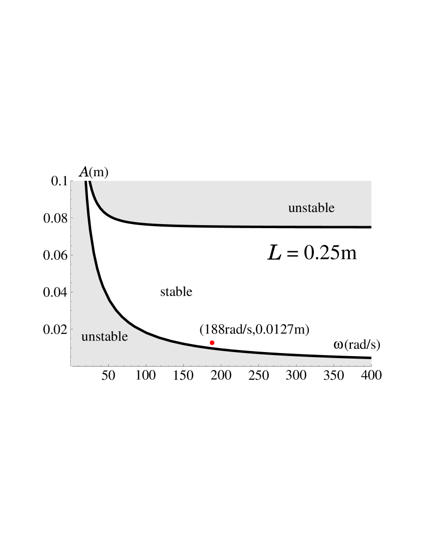
Figure 3 displays the regions of stability of the Mathieu functions plotted in terms of the pendulum drive parameters $A$ and $\omega$ with $L=0.25$ m.m17q The lower smooth curve in Fig. 3 is approximately $A\omega=1.81$ m/s. Note that we should avoid large driving amplitudes ($A>0.08$ m) for a 25 cm rod. The effective potential technique of Ref. Landau, is not valid for large excursions from equilibrium, so does not address an upper stability limit. A numerical solution of Eq. (7) is needed to explore shorter rods (or large driving amplitudes) together with slow oscillation angular amplitudes larger than the linear approximation supports.

A full numerical solution of Eq. (7), including ad hoc frictional damping, for $\theta_{d}=180^{\circ}$ is shown in Fig. 4. Constant friction gives a rapid linear decrease in the oscillation amplitude, while viscous damping gives the familiar under-damped oscillation with an exponentially decreasing amplitude. Our demonstration pendulums seem to be better described by constant friction.

Figure 5 shows interesting, non-oscillatory behavior which appears in numerical solutions for very short rods. This possibly chaotic non-oscillatory behavior of the driven pendulum suggests other studies of overdriven parametric systems which can be simply related to a driven mechanical pendulum. Previous studiesBD ; RLK could easily be extended to arbitrary drive angles using the analysis in Sec. V.

IV.3 Drive angle 90 degrees

For a drive angle $\theta_{d}=90^{\circ}=\pi/2$, the equation of motion for slow oscillations, Eq. (15), reduces to a simple form:

$$\ddot{\phi}+\big{(}{{3g}\over{2L}}-{{9A^{2}\omega^{2}}\over{8L^{2}}}\cos\phi\big{)}\sin\phi=0.$$ (27)

For small angles $\phi$ ($\cos\phi\sim 1$ and $\sin\phi\sim\phi$), we obtain

$$\ddot{\phi}+{{3g}\over{2L}}(1-R)\phi\simeq 0.$$ (28)

Equation (28) gives small oscillations near $\phi=0$ only if $\omega<\omega_{c}$ or $R<1$. However, if $\omega>\omega_{c}$ ($R>1$), the term in parentheses in Eq. (28) is negative, and there cannot be stable oscillation near $\phi=0$. To find the new location of the stable equilibrium angle ($\phi_{0}$), we take $\phi=\delta+\phi_{0}$ in Eq. (27) and write

$$\ddot{\delta}+{{3g}\over{2L}}[1-R\cos(\delta+\phi_{0})]\sin(\delta+\phi_{0})=0.$$ (29)

We obtain the equilibrium angle $\phi_{0}$ by taking $\delta=0$ and $\ddot{\delta}=0$:

$$(1-R\cos\phi_{0})\sin\phi_{0}=0.$$ (30)

The solution $\phi_{0}=0$, which we have already seen, is stable only if $\omega<\omega_{c}$ ($R<1$). Equation (30) also has a second solution valid for $R>1$:

$$1-R\cos\phi_{0}=0.$$ (31)

The equilibrium angle $\phi_{0}$ is nonzero and finite for $R>1$:

$$\phi_{0}=\cos^{-1}{1\over R}.$$ (32)

Observe that $0<\phi_{0}\leq\pi/2$ for $R>1$ (or $\omega>\omega_{c}$).

Near equilibrium this second solution should reduce Eq. (29) to an approximate harmonic oscillator:

$$\ddot{\delta}+\omega_{p}^{2}\delta\simeq 0.$$ (33)

Equation (33) gives a stable equilibrium only if the coefficient of $\delta$ is positive.

$${d\over{d\delta}}\big{\{}[1-R\cos(\delta+\phi_{0})]\sin(\delta+\phi_{0})\big{\}}_{\delta=0}>0,$$ (34)

which yields

$$[1-R\cos\phi_{0}]\cos\phi_{0}+R\sin^{2}\phi_{0}>0.$$ (35)

The requirement for equilibrium at $\phi_{0}$ in Eq. (30) makes the first term in Eq. (35) zero. Hence

$$R\sin^{2}\phi_{0}>0,$$ (36)

which holds for all $0<\phi_{0}\leq\pi/2$ ($\omega>\omega_{c}$ or $R>1$).

Figure 6(a) shows the effective potential for $R=1.75$ with a stable minimum at $\phi_{0}=55^{\circ}$. The effective potential for $R=0.75<1$ is shown in Fig. 6(b), where the only minimum in the potential is at $\phi_{0}=0$.

The horizontally driven pendulum ($\theta_{d}=90^{\circ}$) is stable hanging down ($\phi_{0}=0$) for $R<1$, and stable near $\phi_{0}=\cos^{-1}(1/R)$ for $R>1$.

V The Driven Pendulum at Any Angle

We start with the equation of motion (16) for a general drive angle $\theta_{d}$.

$$\ddot{\phi}+{{3g}\over{2L}}\big{(}\sin\phi+{R\over 2}\sin[2(\phi-\theta_{d})]\big{)}\simeq 0.$$ (37)

Equilibrium occurs when $\phi=\phi_{0}$ with $\ddot{\phi}=0$:

$$\sin\phi_{0}+{R\over 2}\sin[2(\phi_{0}-\theta_{d})]=0.$$ (38)

As we have seen, the equilibrium is stable if

$${d\over d\phi}\big{(}\sin\phi+{R\over 2}\sin[2(\phi-\theta_{d})]\big{)}_{\phi=\phi_{0}}>0,$$ (39)

which gives

$$\cos\phi_{0}+R\cos[2(\phi_{0}-\theta_{d})]>0.$$ (40)

Small oscillations about the equilibrium angle $\phi_{0}$ have the angular frequency $\omega_{p}$, where

$$\omega_{p}=\omega_{0}\sqrt{\cos\phi_{0}+R\cos[2(\phi_{0}-\theta_{d})]}.$$ (41)

The condition for equilibrium in Eq. (38) can be easily solved numerically for $\theta_{d}$ as a (multivalued) function of $\phi_{0}$. However, we wish to know the stable angle of oscillation $\phi_{0}$ as a function of the drive angle $\theta_{d}$. Simply finding the solutions of Eq. (38) is not sufficient. The zeroes must correspond to real angles and to stable equilibriums as defined by Eq. (40). Also, the ideal problem shown in Fig. 1 has a two-fold ambiguity of drive angles at $\theta_{d}$ and $\theta_{d}+180^{\circ}$. Real lab or demonstration apparatus will limit the motion of the rod so that we cannot observe oscillations for $|\theta_{d}-\phi_{0}|>90^{\circ}$.

Figure 7(a) shows that a driven pendulumm17q with $R=1.75$ has a range of drive angles for which there are no (nearby) stable equilibrium angles. For all values of $R\geq 2$, there is a stable equilibrium $\phi_{0}$ for all drive angles $\theta_{d}$. The critical case $R=2$ is shown in Fig. 7(b).

For values of $R>2$, the curve representing $\phi_{0}(\theta_{d})$ becomes smooth, tending to a straight line as $R\to\infty$. (But we must beware of an instability appearing at larger drive parameters, equivalent to large $R$. There are practical limits to how large $R$ can be to give a stable driven pendulum in a physical system.) Values of $R$ less than unity gives stable oscillations with $\theta_{d}\neq\phi_{0}$ over the driving angle range $0<\theta_{d}<90^{\circ}$ as shown in Fig. 8.

VI Comparing Theory with Experiment for Any Drive Angle

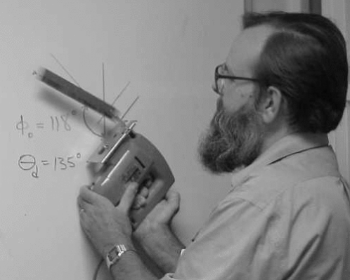
The desire for more degrees of freedom on a limited budget has led us to the driven pendulum demonstration using a small hand-held variable speed jig saw (see Fig. 9). The conversion of the jig saw parameters to the units used here gives the corresponding values of $\omega$ and $A$: $0<\omega<330$ rad/s and $A=0.0089$ m. The $L=20$ cm pendulum gives the expected maximum $R=3.3$, well into the regime where the driven pendulum is stable at all driving angles.

The value of $R$ can be measured using Eq. (32) for $R>1$. Hold the driving saw blade horizontally and measure the angle to which the driven pendulum rises. At low driving speeds, it will oscillate about the downward direction. Once $\omega>\omega_{c}$, the pendulum will slowly rise with increasing drive speed until a maximum angle is reached. Any angle above $60^{\circ}$ will correspond to $R>2$, which then gives stable driven oscillations at any driving angle. The 20 cm pendulum has a measured maximum $\phi_{0}(90^{\circ})\simeq 72^{\circ}$, corresponding to $R\simeq 3.2$, in good agreement with our expectation.

Figure 9 shows the 20 cm pendulum driven with $\theta_{d}=135^{\circ}$ and maximum frequency ($R\simeq 3.2$), having being damped into a steady position near $\phi_{0}(\theta_{d}=135^{\circ})\simeq 118^{\circ}$. Shorter pendulum rods allows the exploration of large $R$, where chaotic motion of the type shown in Fig. 5 may be observed. From simulations and experiments with shorter rods, we find that stable driven oscillations do not extend to very large values of $R$. The unstable system shown in Fig. 5 has a value of $R$ of only 14.5. The upper limit on the amplitude from the Mathieu function analysis described in the Appendix and shown in Fig. 3 does not reliably predict the onset of instability, because the Mathieu equation only applies for small drive amplitudes. The lower limit from the Appendix corresponds to $R=1$. Establishing the correct upper limit on $R$ for stable oscillation requires further study.

VII Conclusions

The pendulum driven at any angle from the vertical has been studied using the effective potential method of Landau and LifshitzLandau for rapid driving angular frequency ($\omega\gg\omega_{p}$). Numerical simulations of the full equation of motion (7) generally confirm the results of the simplified model for $\omega\gg\omega_{p}$. The pendulum will oscillate about the equilibrium angle $\phi_{0}(\theta_{d})$, defined by Eqs. (38) and (40). The angular frequency of small oscillations about equilibrium will occur at $\omega_{p}$ given by Eq. (41).

The general behavior of the driven pendulum at any driving angle is summarized by the parameter $R$ defined in Eq. (19). For $R\leq 1$, there no stable inverted oscillations near $180^{\circ}$. There are stable oscillations with $\phi_{0}>0$ for all $0<\theta_{d}<90^{\circ}$ and $\displaystyle\lim_{\theta_{d}\to 90^{\circ}}\phi_{0}=0$. For $1<R<2$ there are stable inverted oscillations near $180^{\circ}$. Some angles in the range $90^{\circ}<\theta_{d}<180^{\circ}$ are not stable for $|\theta_{d}-\phi_{0}|<90^{\circ}$. Also $\phi_{0}(90^{\circ})>0$. For $R\geq 2$, there are stable oscillations for $|\phi_{0}-\theta_{d}|<90^{\circ}$ for all $\theta_{d}$.

All parameters of the driven pendulum are accessible over interesting ranges with simple and inexpensive apparatus. Even $g$ can be reduced by tipping the plane of oscillation. We have explored more parameter sets than reported here and hope that others will explore and report their own variations of the driven pendulum at angles other than $0^{\circ}$ or $180^{\circ}$.

Appendix A Approximate Analytic Solution of the Inverted Pendulum

Section IV.2 introduced the solution of the inverted pendulum based on the effective potential approach of Ref. Landau, . This system also can be easily solved by linearizing the equation of motion as in Ref. DCM, .

For small angles the equation of motion for the driven inverted pendulum, Eq. (7), simplifies to

$$\ddot{\delta}+\big{(}{{3A\omega^{2}}\over{2L}}\cos\omega t-{{3g}\over{2L}}\big{)}\delta\simeq 0.$$ (42)

Equation (42) has the form of Mathieu’s differential equationAS :

$${{d^{2}y}\over{dz^{2}}}+(a-2q\cos 2z)y=0.$$ (43)

If we make the substitution $z=\omega t/2$, Eq. (43) can be expressed in the Mathieu form,

$${{d^{2}\delta}\over{dz^{2}}}+(-{{6g}\over{L\omega^{2}}}+{{6A}\over{L}}\cos 2z)\delta=0.$$ (44)

The Mathieu parameters can be found by comparing Eqs. (43) and (44) and are $q=-3A/L$ and $a=-6g/(L\omega^{2})$.

The general solutions of Mathieu’s differential equation are expressed by the even and odd Mathieu functions. For a portion of the parameter space in $(a,q)$, the Mathieu functions are real and periodic, corresponding to stable equilibrium of the inverted driven pendulum. Outside of this portion of the parameter space, the functions are complex and divergent, corresponding to unstable oscillations.

The region of parameter space that gives stable oscillations is defined through the Mathieu parameters $a$ and $q$.AS

$$1-|q|-{{q^{2}}\over 8}+{{|q|^{3}}\over{128}}-{{q^{4}}\over{1536}}-{{11|q|^{5}}\over{36864}}+\cdots=a_{1}(q)>a.$$ (45)

$$a>a_{0}(q)=-{{q^{2}}\over 2}+{{7q^{4}}\over{128}}-{{29q^{6}}\over{2304}}+\cdots$$ (46)

For the demonstration pendulum of Ref. m17q, , we have $q=-3A/L=-0.1524$, so $q^{2}\ll 1$. Then, to a good approximation the lower limit from Eq. (46) simplifies to the leading term.

$$a=-{{6g}\over{L\omega^{2}}}>-{{q^{2}}\over 2}=-{{(3A/L)^{2}}\over 2}.$$ (47)

If we solve for the minimum angular frequency for stable inverted driven oscillations, we obtain the familiar result of Eq. (19):

$$\omega>\omega_{c}=\sqrt{{{4gL}\over{3A^{2}}}}.$$ (48)

Including the $q^{4}$ correction from Eq. (46) increases $\omega_{\rm c}$ by less than 1%. The actual apparatus does not warrant this level of precision, so we can safely devise a stable driven inverted pendulum using $A\omega>\sqrt{4gL/3}$.

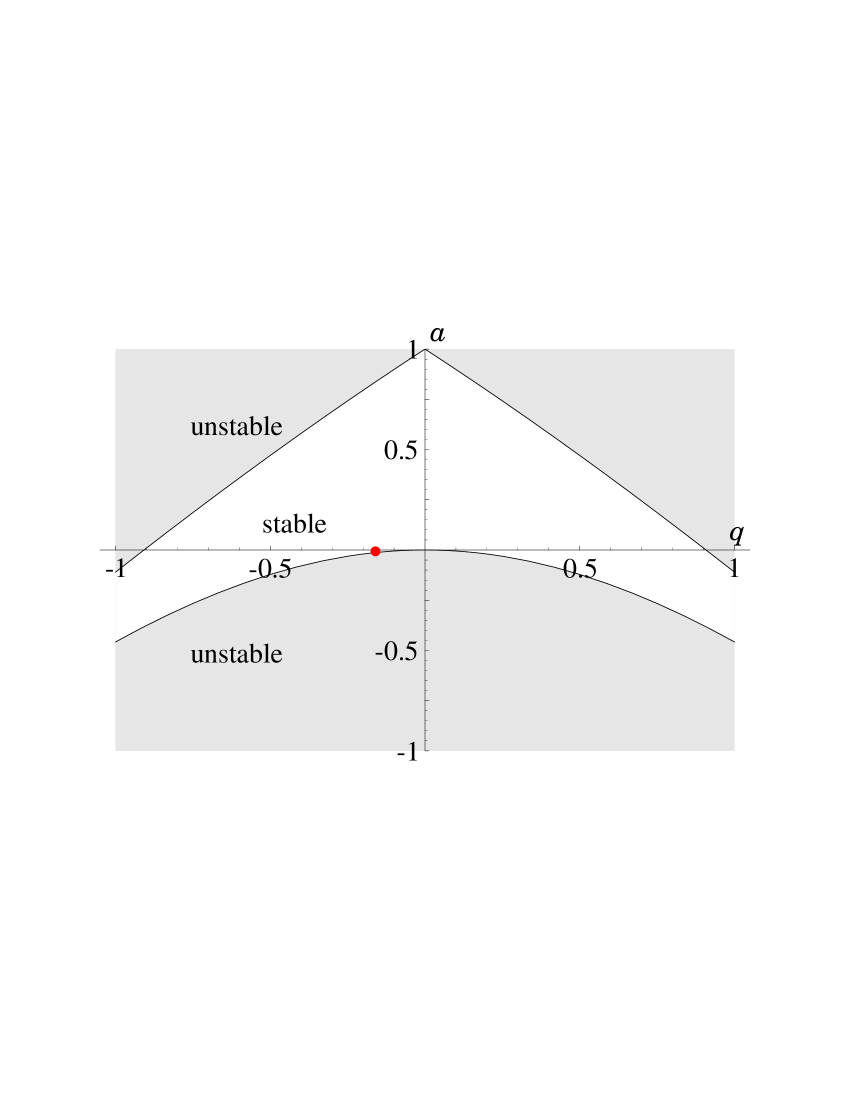
Figure 10 is commonly used to display stable regions in the Mathieu parameter space of $(a,q)$. It is more useful for our purposes to transform to the drive parameter space of $(A,\omega,L)$. The inversion of the first few terms of Eqs. (45) and (46) for $a_{0}(q)$ and $a_{1}(q)$ gives lower and upper limits for the drive amplitude $A$ as a function of the drive angular frequency $\omega$ and the pendulum rod length $L$.

$$A>A_{0}(\omega,L)={L\over 3}\sqrt{{{64-\sqrt{4096-3584{{6g}\over{L\omega^{2}}}}}\over{14}}}$$ (49)

$$A<A_{1}(\omega,L)={L\over 3}\bigg{(}-2+\sqrt{2}\sqrt{3+{{6g}\over{L\omega^{2}}}}\bigg{)}.$$ (50)

These equations were used to generate the limits of stability in the parameter space $(A,\omega)$ for $L=0.25$ m shown in Fig. 3.

Figure 1: The pendulum driven at angle $\theta_{d}$.

Figure 2: The potential $V_{\text{eff}}(\phi)$ for a driven inverted pendulum ($\theta_{d}=180^{\circ}$).

Figure 3: The stable region in the drive amplitude $A$ and angular frequency $\omega$ for a driven inverted pendulum of length $L=0.25$ m. The parameters of the pendulum of Ref. m17q, are shown as a point at $A=0.0127$ m and $\omega=188$ s^-1.

Figure 4: Motion for $\theta_{d}=180^{\circ}$ with constant frictional damping.

Figure 5: Over-driven inverted pendulum of the type modeled in Fig. 4, with $L=0.03$ m. No stable solution is found in the model or is observed experimentally.

Figure 6: (a) Minimum of the effective potential $V_{\text{eff}}(\phi)$ for $R=\omega^{2}/\omega_{c}^{2}=1.75$ at $\phi_{0}\simeq 55^{\circ}$; the equilibrium at $0^{\circ}$ becomes unstable. (b) For $R=0.75$ ($\omega<\omega_{c}$), the only minimum in $V_{\text{eff}}(\phi)$ is at $\phi_{0}=0$.

Figure 7: All equilibriums (dashed) and stable equilibriums (solid line) are shown in $\phi_{0}$ versus $\theta_{d}$ for (a) $R=1.75$, and (b) $R=2$.

Figure 8: All equilibriums (dashed) and stable equilibriums (solid) are shown in $\phi_{0}$ versus $\theta_{d}$ for $R=0.90$.

Figure 9: A driven rod pendulum with $R=3.2$ and $\theta_{d}=135^{\circ}$ displaying stability at $\phi_{0}\simeq 118^{\circ}$.

Figure 10: The stable region in the Mathieu parameters $a$ and $q$ for a driven inverted pendulum. The parameters of the pendulum of Ref. m17q, are shown as a point at $q=-0.00665$ and $a=-0.1524$.