Interaction between dust grains near a conducting wall
Abstract
The effect of the conducting electrode on the interaction of dust grains in a an ion flow is discussed. It is shown that two grains levitating above the electrode at the same height may attract one another. This results in the instability of a dust layer in a plasma sheath.
1 Introduction
A good deal of experiments in dusty plasma physics are performed with aerosol grains suspended in the plasma sheath. A negatively charged dust grain in the sheath levitates above a horizontal electrode due to the balance of two forces: the gravity force directed downwards and the sheath electric field that pushes the grain upwards. The near-sonic or the supersonic ion flow in the sheath creates the wake field downstream of the grain. Since the latter is confined by a certain Mach cone, it is commonly accepted that the wake field affects the motion of grains, which are situated downstream only. The usual assumption is that the intergrain potential is smooth in the horizontal direction, i.e., two grains levitating at the same height repel one another via the screened Coulomb potential. The structure of the wake field and the grain interaction in an ion flow were studied in details [1-5]. The asymmetric interaction of vertically aligned grains was also observed experimentally [6].
Analytical theory and computer simulations cited above assumed that the plasma density is constant and the influence of the conducting electrode is negligible. Although both assumptions evidently fail under conditions of a real plasma sheath, taking into account the plasma non-uniformity seems to be a very difficult problem. In order to estimate the influence of the electrode upon grain interaction, here I use the zeroth approximation, which however, seems the only one treatable analytically.
In the present paper, the following simple model is accepted. Let there be the monoenergetic ion stream entering a conducting electrode (or a grid) located at the horizontal plane, . The stream velocity, , exceeds the ion thermal velocity but it is much less than the electron thermal velocity. Electrons are Boltzmann distributed. Two problems are addressed: first, how does the electrode modify the interaction between two grains levitating at the same height and, second, how this affects the spectrum of dust acoustic waves propagating along a single dust layer.
2 Intergrain interaction
The electrostatic potential produced by a point charge, , located at is given by the solution of the Poisson equation
| (1) |
where is the operator of the static dielectric permittivity of an ambient plasma. Within the accepted model, the spatial Fourier transform of is given by
| (2) |
where is the velocity of the ion flow, is the ion plasma frequency and is the inverse electron Debye length. The ion flow is parallel to the axis and directed downwards, .
In unbounded plasma, the natural boundary condition for Eq. (1) is . It is convenient to express the solution to Eq. (1) in terms of its Green function, i.e., , where the Fourier transform of with respect to the transverse coordinate is
| (3) |
Here stands for the transverse components of a wave vector. With the dielectric function given by Eq. (2), the zeros of denominator in Eq. (3) are
| (4) |
where
| (5) | |||||
| (6) |
is the normalized transverse wave vector, and is the inverse Mach number.
The integral in Eq. (3) is readily evaluated resulting in
| (7) |
The spatial structure of the potential is recovered by the Fourier transform of the Green function (7) with respect to . The first term in parenthesis in expression (7) gives rise to the Debye-Hückel potential distorted by the ion flow, while the second term represents the wake field situated downstream of the charge [1-3]. The opening of the Mach cone confining the wake and the field structure inside it depend on the stream velocity.
Now we turn to the evaluation of the electric potential of a charge located near a conducting wall. Let the wall be situated at plane, while the charge is placed above it, . Then the potential is given by the solution of Eq.(1) supplemented with the boundary condition . As it is well-known from electrostatics, we can make allowance for this boundary condition by introducing the surface charge density, , induced at the conducting surface. Then, the potential of a unit charge is written as
| (8) |
Taking into account the boundary condition, , we find the surface charge density and, finally,
| (9) |
One may doubt whether description a bounded dispersive medium in terms of the response function of an unbounded medium is justifiable. However, more accurate and lengthy calculations give the same result. The physical reason is that there are no ions reflected by the conducting wall within the present model. The mathematical reason is that Eq. (1) actually masks a set of partial differential equations with two real characteristics directed downwards.
Of particular interest for the following is the interaction potential of two charges placed at the same height, . Since
| (10) |
where , the normalized potential is
| (11) |
where and . The asymptotic behaviour of is determined by Eq. (10) at . The latter depends essentially on whether the the ion flow is supersonic or subsonic. In the case of the supersonic flow, , the roots (5,6) at are approximated as
| (12) |
and the leading term of the asymptotic expansion of (11) is
| (13) |
This expression may be interpreted as a mirror reflection of the wake field produced by the grain at . More detailed numerical investigation of the potential (13) shows that is always positive for .
| (14) |
while the potential at infinity behaves like
| (15) |
The most important distinction between the expressions (13) and (15) is that in the subsonic regime the potential is attractive if
| (16) |
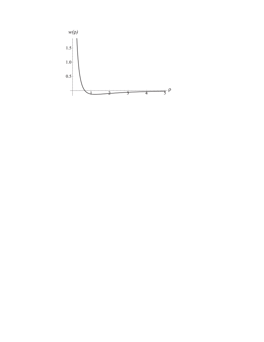
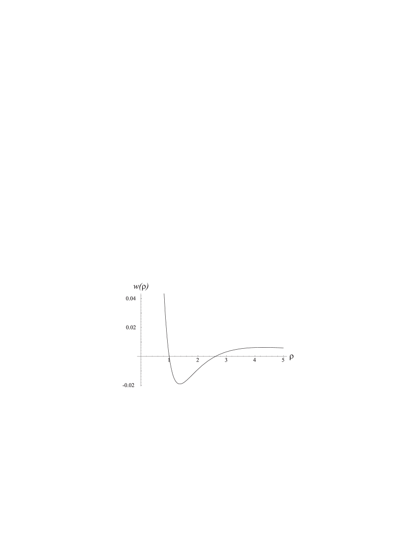
The numerically evaluated example of the potential (15) demonstrating the attraction is depicted in Fig. 1. It should be pointed out that the inequality (16) guarantees the long-scale attraction between grains. With the opposite inequality imposed on and , the potential is repulsive at large distance but the attractive branch may appear at smaller scales, as shown in Fig. (2).
Evidently, the existence of the attractive branch of the interparticle interaction may result in formation of various patterns and clusters even in the absence of the external potential well confining grains in the horizontal direction. Also, the even distribution of grains in a dust layer may become unstable. The latter possibility is discussed in the next section.
3 Dust layer
Now consider a two-dimensional gas consisting of dust grains hovering over the conducting electrode. Ignoring intergrain correlations, the linearized equations of motion are written as
| (17) | |||||
| (18) |
where is the unperturbed value of the surface density and is the density perturbation. Here I consider horizontal motions only, i.e., . The term in Eq. (18) corresponds to the grain friction on an ambient neutral gas. The intergrain interaction is described by the potential given by Eqs. (11). Although the grain charge, , generally depends on the ambient plasma parameters, for simplicity we ignore its variability.
Assuming that all quantities are proportional to we easily get the dispersion relation for the gas oscillations:
| (19) |
where .
This expression describes dust sound waves in the continuous medium approximation. In the long-wave limit, , the dispersion relation is of the form
| (20) |
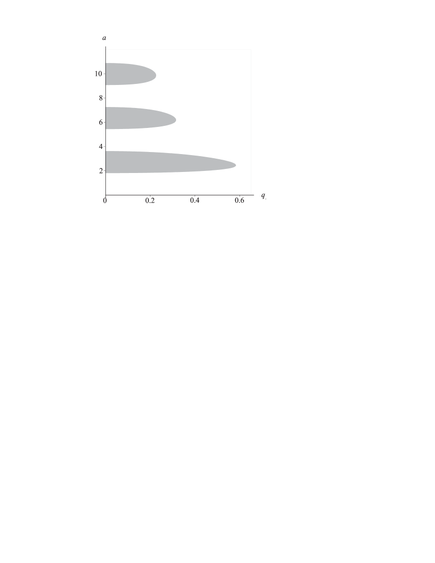
Evidently, the layer is unstable, i.e., , if . In the long-wave limit this is possible in the subsonic flow only and the corresponding constraint coincides with Eq. (16). More detailed investigation shows that the potential, , is always positive if . However, in the subsonic regime, , there are regions of instability, that is, if . The latter are shown as shadowed areas in Fig. 3. With the increasing distance () to the wall or decreasing stream velocity () the instability regions shrink to zero, .
4 Conclusion
To summarize, we have shown that the presence of the conducting wall may drastically change the electrostatic interaction of the dust grains in an ion flow. In particular, the electrostatic image of the grain wake field may result in attraction between grains levitating at the same height that, in its turn, yields the Jeans-type instability of the dust layer.
It would be unduly naive to draw quantitative conclusions from the present calculations. However, it seems reasonable that even in a real plasma sheath, which is essentially non-uniform, the electrostatic image of the grain wake field may also affect the motion of another grains outside the Mach cone. Although in most experiments the screened Coulomb interaction is observed, there are indications that the intergrain potential may be more complicated. It was recently reported that, under certain conditions, a void, i.e., a dust-free region, appears in a central part of a single dust layer [7]. The emergence of a two-dimensional void in a layer consisting of some hundreds of grains can hardly be explained in the same manner as a three-dimensional void; the latter requires strong influence of the dust component upon the discharge structure [8]. Although currently one cannot exclude that some additional external forces appeared in the experiment [7], we can conjecture that the 2D void formation is provided by complicated intergrain interaction, for example, the one described in this paper.
Acknowledgements
This study was supported in part by the Russian Foundation for Basic Research (project no. 02-02-16439) and the Netherlands Organization for Scientific Reseach (grant no. NWO 047.008.013).
References
- [1] M. Nambu, S.V. Vladimirov, and P.K. Shukla, Phys. Lett. A 203, 40 (1995).
- [2] S.V. Vladimirov and M. Nambu, Phys. Rev. E 52, R2172 (1995).
- [3] O. Ishihara and S.V. Vladimirov, Phys. Plasmas 4, 69 (1997).
- [4] G. Lapenta, Phys. Rev. E 62, 1175 (2000).
- [5] G. Lapenta, Phys. Rev. E 66, 026409 (2002).
- [6] A. Melzer, V.A. Schweigert, and A. Piel, Phys. Rev. Lett. 83, 3194 (1999).
- [7] Paeva G.V., Dahiya R.P., Stoffels W.W., Stoffels E., and Kroesen G.M.W., 2D voids in argon, oxygen and argon-oxygen dusty plasmas, 3rd Int. Conf. on the Physics of Dusty Plasmas, ICPDP-2002, 20-24 may 2002, Durban, South Africa
- [8] D. Samsonov and J. Goree, Phys. Rev. E 59, 1047 (1999).