Dynamical transitions in the evolution of learning algorithms by selection

Abstract

We study the evolution of artificial learning systems by means of selection. Genetic programming is used to generate a sequence of populations of algorithms which can be used by neural networks for supervised learning of a rule that generates examples. In opposition to concentrating on final results, which would be the natural aim while designing good learning algorithms, we study the evolution process and pay particular attention to the temporal order of appearance of functional structures responsible for the improvements in the learning process, as measured by the generalization capabilities of the resulting algorithms. The effect of such appearances can be described as dynamical phase transitions. The concepts of phenotypic and genotypic entropies, which serve to describe the distribution of fitness in the population and the distribution of symbols respectively, are used to monitor the dynamics. In different runs the phase transitions might be present or not, with the system finding out good solutions, or staying in poor regions of algorithm space. Whenever phase transitions occur, the sequence of appearances are the same. We identify combinations of variables and operators which are useful in measuring experience or performance in rule extraction and can thus implement useful annealing of the learning schedule. We also find combinations that can signal surprise, measured, on a single example, by the difference between prediction and the correct output. Structures that measure performance always appear after those for measuring surprise. Invasions of the population by such structures in the reverse order were never observed.

PACS numbers: 05., 84.35.+i, 87.23.Kg

Abstract

I Introduction

In this paper we consider the dynamics of automatic design of learning algorithms for neural networks. We use Genetic Programming (GP) as a tool to generate a sequence of generations of populations of programs which implement a learning algorithm. Programs at one generation give rise through cross over and mutations to offspring programs in the next generation according to their fitness. The fitness -which defines the problem- is related in this study to the efficiency of the learning algorithm implemented by the program. We choose a measure of efficiency based on the ability of generalization, related to the expected error of the output on examples which are statistically independent from the training set.

Although GP is similar in spirit and actually inspired by the Genetic Algorithm (GA) of Holland [1], since both mimic natural evolution, the idea of GP put forward by Koza [2], differs from GA in very important ways. GP deals with programs, represented by strings of symbols -variables or functional operators- which can have as inputs different types of variables and operators across the population, as well as along the generations. In some loose sense GP allows for great variability and thus for the emergence of more of something that could be dubbed complexity.

Usually the automatic design of programs has as an aim the solution of a problem and a measure of how far a given candidate goes in that direction is given by the fitness. We are not only interested in final results, but rather the road towards that goal and its characterization are the main issues. We have chosen to study perceptron learning, a sufficiently simple learning problem that can be studied, as far as final results are concerned, by analytical means but which presents a wealth of interesting results. By analyzing the development of learning algorithms we expect to learn something about the dynamics along which different variable combinations become useful and invade the population of programs. We find dynamic phase transitions as different functional structures change from being irrelevant to useful and find evidence that point to a strict temporal order in the sequence of such appearances. Some structures, though useful at later stages are irrelevant at first and remain so until some other structure is mature enough and thus potentialize the utility of the former.

The characterization of a population can be made through the use of several different complementary tools. What we call the phenotypic or functional level description deals with quantities that measure the expression of important traits. At this level the program differences are irrelevant as long as they give rise to the implementations of the same function. The main tool, the phenotypic entropy $S$ describes the distribution of fitness in the population. At the genotypic or program level, different programs are different even if they give rise to the same numbers, for their potential of generating new successful programs in the following generation depends on the particular symbols which exist at present. We can introduce several genotypic entropies which describe the distribution of probabilities of symbols, of two contiguous symbols and so on. We will restrict to dealing with single symbol distributions and we characterize them by $H$ the genotypic entropy [3].

The crossover of programs, obtained by a cutting and pasting process described bellow, can be difficult to implement in common programming languages such as C and Fortran. The major part of the work in GP has been developed in LISP which is also the case in this study. We have developed also a protocol for simulation of LISP on a parallel architecture on a cluster of machines running Linux, which is described in [4].

The paper is organized as follows. In section 2 a brief description of GP from the very special point of view which interests us here is followed by a description of the problem which GP aims at solving. Section 3 presents the results and concluding remarks can be found in the last section.

II The problem and the method

A Problem: Learning by a perceptron

The learning problem to be analyzed by the GP must strike a balance between being complex enough so that interesting dynamics arises and simple to the point that details can be understood and simulations performed. The perceptron meets these demands and has a long and distinguished history. For an extensive view from a Statistical Mechanics perspective see [5]. We consider the realizable teacher-student learning scenario. The perceptron classifies vectors ${\bf S}\in{\rm I}\!{\rm R}^{N}$ (here obtained i.i.d from a uniform distribution) in two categories with labels $\sigma_{{\bf J}\mu}=\pm 1$ according to the rule $\sigma_{{\bf J}\mu}={\rm sgn}({\bf J}\cdot{\bf S})$. The objective of the learning dynamics is to determine the weight or synaptic vector ${\bf J}\in{\rm I}\!{\rm R}^{N}$ from pairs of examples $({\bf S}_{\mu},\sigma_{\mathbf{B}\mu})$ which carry information about a rule. We restrict ourselves to the simplest case of noiseless realizable rules, which mean that the labels were uncorrupted and generated by another perceptron with a weight vector ${\bf B}\in{\rm I}\!{\rm R}^{N}$ unknown to us. We consider on-line learning, which means that ${\bf J}$ will be built sequentially by modifications induced by the arrival of new pairs of examples. We even concentrate on the particular form of modulated Hebbian learning, where the increments of ${\bf J}$ are described by a modulation function $f$, thus $\Delta{\bf J}_{\mu}={\bf J}_{\mu}-{\bf J}_{\mu-1}=f\,\sigma_{\mathbf{B}\mu}{\bf S}_{\mu}/\sqrt{N}$. This is not very restrictive as a large fraction of the previously studied algorithms, both on-line and off-line, may be put in a similar way and in the (thermodynamic) limit of large networks it can represent asymptotically efficient learning, which even saturate Bayesian bounds.

We deal with questions about the modulation function, such as : (i) What are the variables upon which the modulation function depends? (ii) What is the best function? (iii) In the event that the machine has no access to all of the useful variables, which ones can be left out and which are relevant? That is, in the path towards the development of a more sophisticated algorithm, the machines at earlier stages may not dispose all relevant variables, then which are the ones that are relevant in the earlier stages and which become so later? Is there any discernible pattern in the order these variables are incorporated? That we can indeed identify such time ordering in our simulations is the main result of this paper.

Related questions have been addressed before [6], see: about best results and Bayesian bounds [7], for a variational point of view about the perceptron learning in [8], about feedforward architectures with hidden units in [9, 10, 11], for drifting rules in [12, 13], in an unsupervised scenario [14], from a more general Bayesian perspective in [15, 16, 17]; in the case of off-line learning in [7, 18]. From the perspective of time ordering it has been discussed in [19].

B Method: Algorithm construction by Genetic Programming

In this section we describe briefly our implementation of GP for the problem at hand. We do not consider the evolution of machine architecture, which is left for future work and just deal with the evolution of the modulation function.

Conventional GA work manipulating fixed-length character strings that represent candidate solutions of a given problem. For many problems, hierarchical computer programs are the most natural representation for the solution. Since the size and the shape of the program that represents the solution are unknown in advance, the program should have the potential of changing its size and shape. The aim of GP is getting computers to program themselves by providing a domain independent way to search the space of possible computer programs, for one that solves a given problem. The principle that rules GP is, as in GA, the survival of the fittest.

Starting from a population of randomly created computer programs, the GP operations are used to generate the population of the next generation. The programs are ranked by their fitness and then the GP operations are applied again. These two steps are then iterated.

The most common computer language used in GP is LISP, therefore we will refer to the population individuals as programs or LISP S-expressions indistinctly. We call Faithful S-expressions (FSEs) a lists of symbols that do not return an error message when evaluated. Components, also called atoms, of the S-expressions can be either functional operators or variables. The set of all operators used in the S-expressions is ${\cal F}$ and the set of all variables is ${\cal V}$. The choice of these sets depends on the nature of the problem being faced. For instance, if the solution of a problem can be represented by a quotient of polynomials, ${\cal F}$ = {+ - * /} and ${\cal V}$ = {x 1}. For example, a FSE is (+ (+ x x) (* x (- x (- x x)))), which is a (non unique) LISP representation of the function $2x+x^{2}$. The simplest FSE is an operator followed by the appropriate number of variables (two in the example above). All FSEs have an operator as first element, and following elements should be variables or FSEs. Unfaithful S-expressions are for instance: (x x), (+ x *) and (x - x).

LISP’s most prominent characteristic with regard to GP is that programs and data have a common form and are treated in the same manner. This common form is equivalent to the parse tree for the computer program and allows to genetically manipulate the parts of the program (i.e., subtrees of the parse tree).

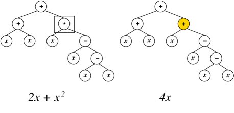
FIG. 1.: LISP programs as parsing trees before and after a GP mutation. A randomly selected atom in the parse tree is changed to another randomly selected atom of the same type. In this example a multiplication operation is replaced by an addition.

The GP operations considered in the present work are asexual reproduction, mutation and cross-over. In the operation of asexual reproduction a certain fraction of the top ranked individuals are copied without any modification into the new generation, ensuring the preservation of structures that made them successful. Mutation is implemented by randomly changing an atom of an individual chosen at random. The new and old atoms must be of the same kind to ensure faithfulness. Finally the modified tree is copied into the new generation. In order to accelerate the dynamics different mutation rates can be used for different atom types. Although there are no sexes associated to the programs, cross-over can be better described as the sexual GP operation. In our experiments, the first parent is chosen among the reproduced fraction of the population (those programs that have been copied from the past generation) by tournament [2]. The second parent is chosen by tournament among the entire population. An atom is selected randomly in each parent. The subtrees (or leaves) with roots in the selected atoms are interchanged to generate two offsprings. In order to avoid uncontrolled growth if the depth of any of the offsprings is above a given threshold, the program is deleted.

After a new population is created, the fitness of each individual is measured and so a new ranking is built. There is a great freedom in choosing the fitness function. It is always a macroscopic or phenotypic quantity, i.e. a function of the expressed characters, and although it reflects the microstructure, it is not a function of the genetic details of the individual. Errors in the measurement of the fitness have a bearing on the dynamics, not entirely different from the temperature in simulated annealing.

Our numerical experiments have been performed in a Pentium III, 800 MHz PC, Linux cluster, using the strategy described in [4]. The GP parameters used in the simulation are presented in Table 1. At generation zero a population of 500 faithful S-expressions is created at random. The programs have (in agreement with Table 1) a maximum depth of $7$ nested parenthesis. The sets used to build the programs are

$\displaystyle{\cal V}=\left\{\sigma_{{\bf J}\mu}\;\sigma_{\mathbf{B}\mu}\;h\;{\bf S}_{\mu}\;{\bf J}_{\mu}\right\}\,,$

where $h={\bf S}_{\mu}\cdot{\bf J}_{\mu}/\left\|{\bf J}_{\mu}\right\|$, and

$\displaystyle{\cal F}=\left\{{\sf Psqr\;Pexp\;Plog\;abs\;+\;-\;*\;\%\;p.\;pN.\;ev\!*\;vv\!+\;vv\!-}\right\}\,,$

where Psqr, Pexp, Plog, and % are the protected square root, exponential, logarithm and division; abs, +, -, and * are the usual absolute value, addition, subtraction and multiplication; and p., pN., ev$*$, vv$+$, and vv$-$ are the inner product, normalized inner product, the product of a scalar times a vector, the addition of two vectors and the subtraction of two vectors respectively. Protected functions are functions whose definition domains have been extended in order to accept a larger set of arguments. The definitions of these functions appear in Table 2.

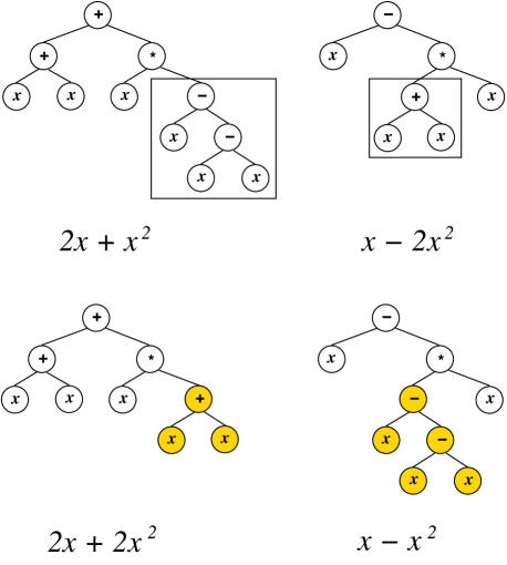
FIG. 2.: GP cross-over. Two parents are selected from the population. A random point in each tree is selected. The branches that grow from the point are interchanged in order to generate two offsprings.

The inner product is the usual inner product among vectors. If ${\bf x}$, ${\bf y}$ $\in{\rm I}\!{\rm R}^{N}$ then the normalized inner product is ${\bf x}\cdot{\bf y}/N$. Other operations involving vectors have to be defined. The ${\sf ev*}$ takes two arguments, a scalar x and a vector $\mathbf{v}$, and returns a vector $\mathbf{w}$ with components ${\sf w}_{i}={\sf x\,v}_{i}$. The sum (difference) of two vectors ${\sf vv+}$ ($\sf vv-$) takes two vectors $\mathbf{v}$ and $\mathbf{w}$, and returns a vector $\mathbf{z}$, with components ${\sf z}_{i}={\sf v}_{i}{\sf+w}_{i}$   $\left({\sf z}_{i}={\sf v}_{i}{\sf-w}_{i}\right)$.

When the process of creation of programs is done, before performing the GP operations to generate the next generation, the fitness has to be calculated. Because the programs represent the learning algorithm of a neural network, a good measure of the learning algorithm performance, should be based on the generalization error, which measures the probability that the classification of the network $\sigma_{{\bf J}\mu}$ is different from the correct label $\sigma_{\mathbf{B}\mu}$

$\displaystyle e_{g}\left(\mu\right)=\left\langle\Theta\left(-\sigma_{\mathbf{B}\mu}\sigma_{{\bf J}\mu}\right)\right\rangle_{{\cal L}_{\mu}},$

which in the thermodynamic limit

$\displaystyle e_{g}\left(\mu\right)=\frac{1}{\pi}\arccos\rho\,,$

where $\rho=\lim_{N\rightarrow\infty}\left(\frac{{\bf J}_{\mu}\cdot\mathbf{B}}{\left\|{\bf J}_{\mu}\right\|\left\|\mathbf{B}\right\|}\right)$ and $\mu$ indicates how many examples have been presented to the network, which we call the age of the individual. The average is over training sets of $\mu$ pairs of examples. Since the aim is to obtain algorithms with the smallest possible generalization error, which depends on the age -taken as the number of examples already to which the network has been exposed- , we chose a fitness that incorporates the variation of $e_{g}$ with age and average over age so that the asymptotic stage is at least as important as earlier stages. For the $k^{th}$ member of the population

$\displaystyle F^{(k)}=\sum^{P}_{\mu=1}\mu e_{g}\left(\mu\right)\,$

is the fitness and $P$ is the total number of examples (maximum age) presented to the network. The population is ranked according to fitness and the best $10\%$ are asexually reproduced into the next generation (according to the Reproduction Rate on Table 1). The other $90\%$ is generated by cross-over. The first parent is chosen from the best $10\%$ of the population. To do so we select first a number $a$ such that $1\leq a\leq P$ with a probability proportional to $a$ (the higher the $a$ the higher the probability to choose it). $a$ is the age of the individuals that are going to participate in the tournament. From the best $10\%$ of the population, ten individuals are selected at random. From comparison of their generalization error at age $a$, the individual with smaller $e_{g}(a)$ is selected for cross-over. To select the second parent a similar mechanism is applied. Ten individuals are selected at random from the entire population, and their generalization errors at age $a$ are compared. The winner is chosen to mate. To perform the cross-over, sub-trees of both parents are selected at random. Internal points (i.e. operators) are selected more frequently than external points (i.e. variables) in order to make the individuals grow (see Table 1).

If either one of the offsprings has a depth bigger than 17, it is deleted. With a mutation rate of 0.01% (one every 20 generations) a mutation is performed to the offsprings. Because the pairs ${\bf J}_{\mu}\,{\bf J}_{\mu}$ become rare after few generations (at the beginning of the simulation, the learning algorithms that use J are not efficient) we keep injecting this pair with a rate of 0.2% (at least one individual per generation receives this pair). Different mutation rates just serve the purpose of accelerating the dynamics and decrease the time scale of the typical time that it takes for interesting things to happen. The process is repeated until the new population reaches the full size fixed here at 500. To calculate the generalization error an average is taken over at least 50 sets of examples ${\cal L}_{P}=\left\{\left(S_{\mu},\sigma_{\mu}\right)\right\}^{P}_{\mu=1}$.

Parameters	Values
Population Size	500
Reproduction Rate	10%
Mutation Rate	0.01%
JJ Mutation Rate	0.2%
Max. Depth Gen. 0	7
Max. Depth Gen. G	17
Prob. Internal Point Select. (cross-over)	90%
Tournament Participants	10
Vector Sizes	11
Maximum Number of Training Examples	100
Maximum Number of Sets of Examples	50
Slave Processors	10
$\beta$	1

TABLE 1. Control parameters for the GP simulation in our experiments.

Function	Definition
(Psqr x)	(sqrt (abs x))
(Pexp x)	(exp (min 13.0 x))
(Plog x)	(log (max 1.d-17 x))
(% x y)	(if ($>$ 1.d-17 (abs y)) 1.d17 (/ x y))

TABLE 2. Definition of the protected function as FSEs. The protected square root is just the square root of the absolute value of its argument. In this manner we extended its domain into the negatives. The exponential is well defined in the reals. Although, in order to avoid overflows we have to impose a cut-off. The protected logarithm has a cut-off at a small positive number to extend its domain to the non-positive numbers. And the protected quotient allows the division by zero (if the absolute value of the denominator is smaller than a tiny number the protected quotient returns a big number, if not it just returns the usual quotient).

III Results

To characterize the distribution of the fitness across the population we introduced the normalized fitness, a measure of the fraction of the total (exponential) fitness that an individual has, in a way analogous to the canonical state at temperature $\beta$ (although the system is not in equilibrium with any temperature reservoir):

$\displaystyle n_{\beta}^{(i)}=\frac{\exp\left(-\beta F^{(i)}\right)}{\sum^{M}_{k=1}\exp\left(-\beta F^{(k)}\right)}\,,$

where $F^{(k)}$ is the fitness measure of th $k^{th}$ individual of the population. Note that smaller values of the fitness are associated to better performances. The use of the exponential amplifies the importance of the individuals with better performance and $\beta$ was kept equal to $1$. We introduce the entropy of the normalized fitness

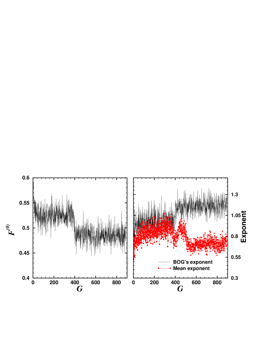
FIG. 3.: (Left) Fitness of the best-of-generation individual of the population vs. the number of generations. A sudden change takes place around 380 generations. (Right) The exponent of algebraic decay of $e_{g}$. Upper curves: BOG, lower curves: population average.

$\displaystyle S=-\sum^{M}_{k=1}n_{\beta}^{(k)}\,\ln\left(n_{\beta}^{(k)}\right)\,,$

a function of the expressed characters of the population (fitness), thus dubbed the phenotypic entropy or Ph-entropy. Note that this entropy is largest when all the members of a population have the same fitness and that the appearance of a distinguished individual, for better or worst, is signaled by a decrease in Ph-entropy.

Each FSE in the population has a well defined length $\lambda^{(k)}$, i.e the number of atoms (operators and variables) that make it up. We define the mean length $L$ as

$\displaystyle L=\frac{1}{M}\sum_{k=1}^{M}\lambda^{(k)}\,.$

To characterize the internal structure of the programs, we estimate for each position $i$ the probability that symbol $s_{q}$ (a variable or an operator) appears at position $i$, $\omega\left(s_{q}|i\right)$ by measuring the frequency over all the population. The genotypic entropy (or G-entropy) which is a function of the micro structure of the individuals in the population is then defined as [3]

$\displaystyle H=-\sum_{s_{q}\in{\cal Q}}\sum_{i}\omega\left(s_{q}|i\right)\,\log_{\left|{\cal Q}\right|}\omega\left(s_{q}|i\right)\,,$

where ${\cal Q}$=${\cal F}$ $\cup$ ${\cal V}$

Several numerical experiments, starting from different random seeds, have been performed using the GP described above.

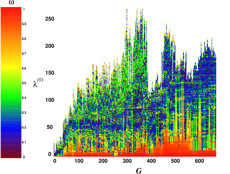
FIG. 4.: Color coded bar graph of the best-in-generation (BOG) individual. The time $G$ is in the horizontal axis is measured in generations and the length of the program is in the vertical axis. Color of pixel at coordinates $(G,i)$ codes for the frequency $\omega\left(s_{q}|i\right)$, according to the color scale, at which the symbol $s_{q}$ (which is the i-th atom of the best-of-generation FSE) appears at position $i$, at generation $G$.

Although the history of the population varies from run to run, we have identified some systematic occurrences.

FIG. 5.: Phenotypic entropy as a function of the number of generations $G$.

In most of the runs we have found a drastic change in behavior which can be well described as a phase transition, although we have neither taken thermodynamic limits associated to infinite network dimension nor infinite population. The time of the occurrence varied widely from one simulation to other. In some simulations, the population did not undergo the transition but it could well happen that we just did not wait long enough. In what follows we consider an illustrative run which presents clearly some features that are typical of other runs. We found a dramatic change of behavior around generation $380$ that can be seen by using several different signatures. Figure 3 (left) shows the fitness of the most adapted program or best-of-generation (BOG) as a function of time. The exponent that governs the decay of $e_{g}$ shows a sharp change, specially if the population average is compared to that of the BOG. Finite size errors are responsible for the fact that exponents larger than one can be found. To understand how representative of the whole population is the BOG we composed a color coded bar graph (see fig. 4) where each vertical bar represents the BOG program written as a string of symbols, time is measured in generations in the horizontal axis. At the position of each symbol in the program a colored square represents the empiric probability of the symbol in the population. Note that quite rapidly an initial symbol is predominant in the population. This is invariantly found in all runs and it is always a symbol that ensures that the modulation function is positive, for other wise the learning would be anti-Hebbian and inefficient. The initial part of the code is very robust and thus is shared by almost all the population. There is an obvious change in the length of the BOG which will be considered bellow, but notice before the transition the upper part is moderately common (green) and after the transition the upper part is more variable or less frequent. These changes can also be monitored by the entropies.

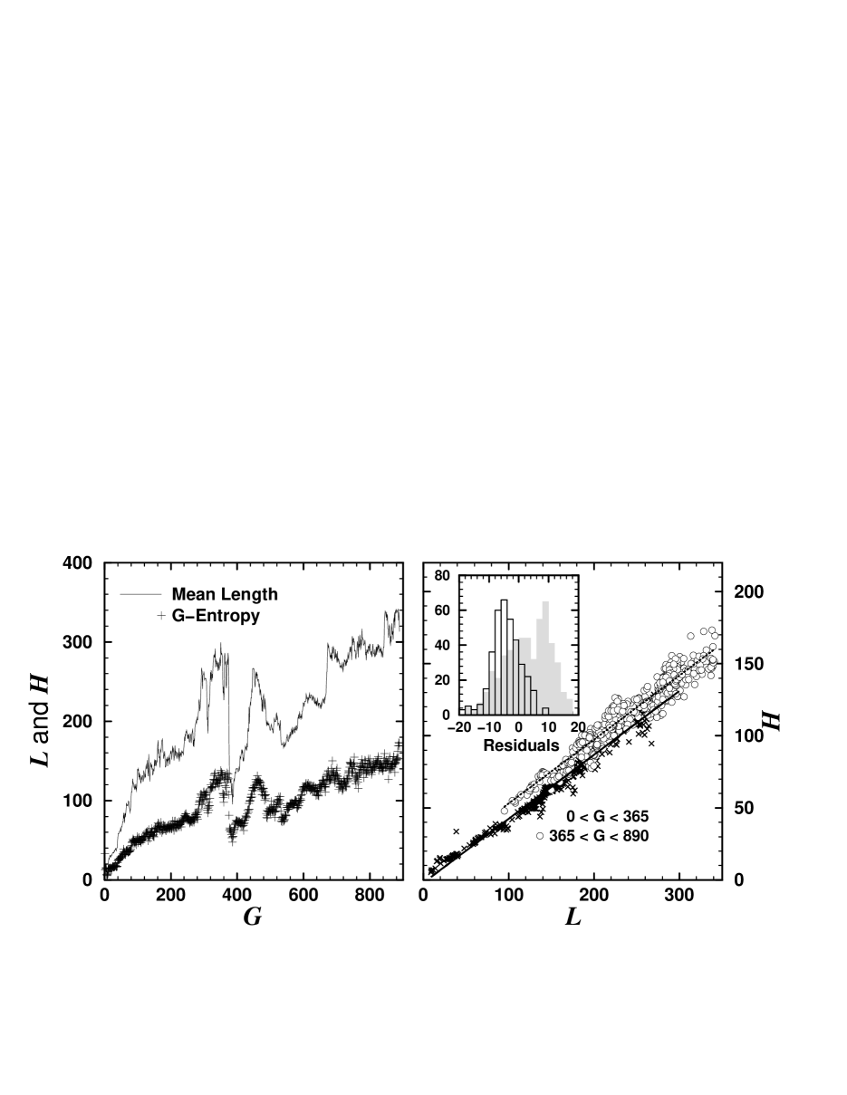
FIG. 6.: (Left) Genotypic entropy and mean length as functions of the number of generations $G$. The transition can be seen by the sharp change around $G=380$. (Right) $H$ vs. $L$. Two linear fits are shown for data before the transition (crosses) and data after the transition (circles). To see that two linear fits are necessary we did a single linear fit of the whole data set and plotted (inset) the histograms of the residuals to the single linear model. The two histograms are for data before and after the transition respectively and the separation of the two peaks lends support to the modeling by two linear regimes.

FIG. 7.: Typical behavior for late stage generation: the length of the weight vector $||{\bf J}||$ increases monotonically when the error of generalization decreases, thus it can be used as a measure of the experience of the individual or of its performance in solving the classification problem. It leads to efficient annealing of the learning rates.

Both entropies (phenotypic and genotypic) present changes about the same time (figs. 5 and 6). The Ph-entropy shows a much larger variability after the transition, the G-entropy and the mean length both have an almost discontinuous break at the transition. The fact that the Ph-entropy has a decreasing trend after the transition can be attributed to the fact that the G-entropy increases and thereby makes the BOG less frequent than immediately after the transition. Now the fitness distribution is sharper around the BOG and therefore the Ph-entropy decreases and oscillates over a wider range.

The G-entropy and the mean length are linearly correlated. This is natural since G-entropy, as defined should be extensive. What is not as expected is the fact that there are two distinct linear regimes before and after the transition. To see this we did a linear fit to the whole data set and plotted an histogram of the residuals, that is the difference between the actual value of a data point and the corresponding value of the linear model. The two histograms in the inset of fig. 6 show clearly a systematic error for the single linear model. These results prove the existence of a quite sharp transition, but do not hint at the nature of the changes in the individual programs nor the reasons for the improvements in fitness. The question is trying to understand what happened from a functional point of view that led to such an improvement in generalization ability.

There are two quantities or functional structures that are of interest both in a quantitative and qualitative analysis of the of learning algorithms. The first, which can be associated to the product $h\sigma_{\mathbf{B}\mu}$ can be functionally described as quantifying a measure of surprise. This is because if $h\sigma_{\mathbf{B}\mu}>0$ the network will classify correctly the example with classification label $\sigma_{\mathbf{B}\mu}$, while if $h\sigma_{\mathbf{B}\mu}<0$, the classification is wrong. Thus it gives a signal of how wrong or correct was the classification and also how stable that classification is under changes of the weight vector. This is obviously an important factor to take into account while incorporating the information in a given example. The second functional structure we will concentrate on is something that can estimate the performance or acquired experience of the network in the implementation of the rule. This, if properly used is akin to annealing of the learning rate or of the functional annealing in learning algorithms. This can be implemented by using the length of the weight vector ${\bf J}_{\mu}$. In fig. 7 we show a graph of $\left\|{\bf J}\right\|$ as a function of the generalization error for a program with a good fitness in the later stages of the simulation. The monotonic behavior is a typical result. It can be shown, at least in the thermodynamic limit, that for algorithms which do not measure surprise their generalization error decays as $\mu^{-1/2}$ and for them annealing is useless. Learning algorithms that use surprise have a better performance $\left(e_{g}\propto\mu^{-1}\right)$ and algorithms that use both surprise and annealing by experience have an even better performance since can have smaller coefficients of $\mu^{-1}$. A crude measure of the capacity of a population of using a functional structure may be given by the frequency that the combination of variables is found. This is admittedly crude since the position in the program determines whether it is useful or not. On the other hand the absence of such combination does not rule out the possibility that some other combination is doing the job in a more cumbersome manner. In fig. 8 we plot the density of pairs $h\sigma_{\mathbf{B}\mu}$ (surprise) and the density of pairs $\mathbf{JJ}$ (performance) in the entire population, as functions of the number of generations.

FIG. 8.: Typical behavior of the density of pairs $h\sigma_{\mathbf{B}\mu}$ and ${\bf J}_{\mu}\,{\bf J}_{\mu}$ as functions of time $G$ measured in generations. Notice the sharp rise at the beginning of the density of $h\sigma_{\mathbf{B}\mu}$ surprise measuring pairs and the later rise of ${\bf J}_{\mu}\,{\bf J}_{\mu}$ , performance measuring pairs. The time ordering is robust and was never seen in the reverse order.

It is possible to observe a fast change in the frequency of pairs of symbols related surprise before 20 generations. $\mathbf{JJ}$ pairs are almost immediately all but extinguished from the population. $h\sigma_{\mathbf{B}\mu}$ pairs are distributed very frequently and its presence oscillates across the population and through the generations, while $\mathbf{JJ}$ pairs introduced by mutations are not able to invade the population. At the time of the transition, surprise is being correctly measured and now the appearance of $\mathbf{JJ}$ leads to an improvement in fitness since it leads to an estimate of the generalization error and permits the implementation of correct annealing schedules. This successful strategy invades the population. It is reasonable to associate the improvement in the fitness with the emergent use of experience by the elements of the population. Notice that injections through mutations of performance structures were non invading before the transition. Of course this can be explained by claiming that not every kind of annealing is beneficial but most important, before surprise is measured correctly, no annealing scheme is useful, and therefore individuals which could measure $\mathbf{JJ}$ did not benefit from such knowledge.

The sequence of symbols of the BOG individual before and after the change in the density of pairs $\mathbf{JJ}$ mirror that increase. In fig. 9 we present the most adapted individual at generations 300, 350, 400 and 450. Just before the transition there is no pair $\mathbf{JJ}$ present in the program (the two first programs). After the transition the best individual suffers a decrease in size and several pairs $\mathbf{JJ}$ appear. According to the color scale, red symbols are extremely frequent in the population at that position, green symbols are just frequent at that position, and violet are quite unlikely to be found. We can see that after the transition, the third program, presents symbols mostly in the violet. 50 generations later there are islands of green in the BOG. That means that the genetic character of the best individual has invaded the population.

A more general analysis of the density of pairs can be done with the help of fig. 10. In these pictures we present the relative frequencies at which each possible pair appear in the population. The vertical axis represents the first element of the pair, the horizontal axis the second element. The size of the white squares represent the frequency of the pair, relative to the most frequent pair (represented by the largest square in each picture). In panel (a) we present the density of pairs at generation 300, (b) corresponds to generation 350, (c) to generation 400 and (d) to generation 450. In (a) and (b) there are no pairs $\mathbf{JJ}$. The most frequent pair is the combination $\sigma_{\mathbf{B}\mu}\sigma_{\mathbf{B}\mu}$, which is just a $1$, but not quite since it can evolve into different directions. After the transition, in panels (c) and (d), this pair remains the most frequent, but important changes have happened. There are small white squares for the pair $\mathbf{JJ}$ representing the emergence of the use of experience by the learning algorithms.

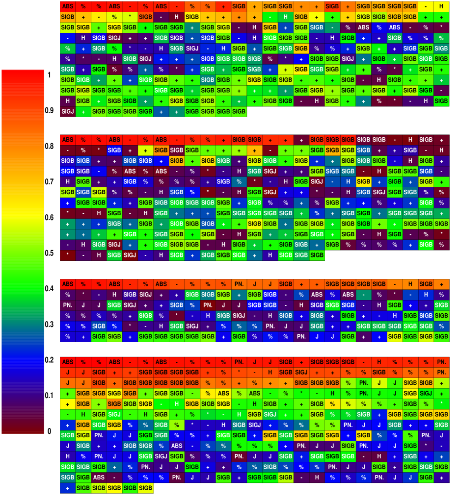
FIG. 9.: The strings of symbols are the programs best-of-generation at generations 300, 350, 400 and 450. The colors represent the frequencies $\omega\left(s_{q}|i\right)$, according to the color scale.

The modulation functions of BOG’s at different stages of the evolution can also be understood along the line of surprise-performance analysis. At earlier stages the BOG is unable to use surprise. Although surprise functional structures are found throughout the population, their incorrect use makes the BOG an annealed Hebbian algorithm. It is known that annealing will not improve the Hebbian learning and the frequency of performance functional structures decreases until it vanishes. It will only appear in very modest ways through mutation and, repeatedly individuals which use it becomes extinct. Later on surprise is finally well accounted for and correctly classified examples cause typically smaller Hebbian corrections than those incorrectly classified. At that point the correct use of surprise potentializes the beneficial use of functional structures that measure performance. Then a correctly annealed algorithm emerges that resembles quite closely the modulation functions found through Bayesian or variational approaches (fig. 11).

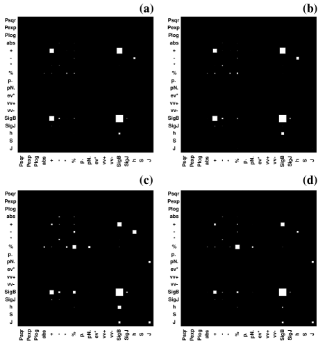
FIG. 10.: Density of pairs for generations 300 (a), 350 (b), 400 (c), and 450 (d). In all the cases the most frequent pair is $\sigma_{\mathbf{B}\mu}\sigma_{\mathbf{B}\mu}$ (SigB SigB). Only in the last two panels the pair JJ appears.

IV Conclusions

Evolutionary programming techniques provide the means to automatically design programs which solve certain class of problems. In this paper, however we were not interested in the final result, the problem that GP was set out to solve has been previously analyzed from many angles and a detailed understanding of online learning in perceptrons has been achieved. Rather we concentrated on the dynamics of evolution and have detected dynamical changes in the behavior of the GP solutions that we have not hesitated in dubbing dynamical transitions. This is not a conventional phase transition associated to singularities arising in the thermodynamic limit. A few runs failed to present the transition, maybe because of time limitations, but it was seen in many different runs. Some features were never reproducible but others were present in every transition. As examples of those features that depend upon contingencies we include the number of generations before the transition takes place, the width of the transitions (some were just about ten generations wide, others took several tens of generations) and the result of the GP, i.e. the program that implements the best learning algorithm. These are mainly important from a constructive point of view when the solution to the problem is the main concern. We tried, instead to identify robust features which can be confidently expected to occur every time the transition takes place. In serving such purpose we have characterized the dynamics by looking at Ph- and G-entropies which give a picture of the distribution of phenotypic fitness and functional or symbolic structure respectively. Large entropic fluctuations are well described by power laws.

FIG. 11.: Modulation functions. (Left) Early stage where surprise is not measured and annealing by experience is ineffective. (Center) Intermediate stage, now surprise is used but annealing by experience has been lost. (Right) Late stage, after the transition, where surprise through the measurement of $h\sigma_{\mathbf{B}\mu}$ and annealing $\left\|{\bf J}\right\|$ are correctly implemented.

The conformation diagram gives a bird’s eye view of the relation of the BOG and the frequency of symbols in the population as well as its length The main robust feature can be identified once the transition has been understood from a functional point of view, in terms of two concepts: the surprise that newly arrived information elicits and how such information should be taken into account based on how much experience the network has in solving the task at hand. A temporal order can be identified in every transition. It was never found otherwise. Performance can be useful only after surprise is measured correctly.

There are several possible extensions of this problem. From a biological point of view there is a suggestive similarity with the time order in which certain structures responsible for measuring surprise and performance have appeared. Will this order be found in more complex artificial settings? Is this biologically significant? Can it be extended to other functional structures? It should also be quite interesting to further analyze phase transitions in the automatic design of programs.

REFERENCES

- [1] J. H. Holland “Adaptations in Natural and Artificial Systems: An Introductory Analysis with Applications to Biology, Control and Artificial Intelligence” U. of Michigan Press, Ann Arbor (1975).
- [2] J. R. Koza “Genetic Programming: on the Programming of Computers by Means of Natural Selection”, MIT Press (1992).
- [3] This is similar to that introduced in C. Adami, C. Ofria, and T. C. Collier, Proc. Nat. sci. USA 97, 4463 (2000), but not restricted to fixed size program length.
- [4] J. P. Neirotti and N. Caticha, available at http://www.fge.if.usp/~nestor/.
- [5] A. Engel and C. Van den Broeck , “Statistical Mechanics of Learning”, Cambridge University Press (2000).
- [6] S. Amari, IEEE Transactions EC-16, 299 (1967).
- [7] M. Opper and D. Haussler, Phys. Rev. Lett. 66, 2677 (1991).
- [8] O. Kinouchi and N. Caticha, J. Phys. A: Math. and Gen. 25, 6243 (1992).
- [9] M. Copelli and N. Caticha, J. Phys. A: Math. and Gen. 28, 1615 (1994).
- [10] R. Vicente and N. Caticha, J. Phys. A: Math. and Gen. 30, L599 (1997).
- [11] R. Simonetti and N. Caticha, J. Phys. A: Math. and Gen. 29, 6243 (1996).
- [12] M. Biehl and Schwarze, J. Phys. A: Math. and Gen. 20, 733 (1993).
- [13] O. Kinouchi and N. Caticha, J. Phys. A: Math. and Gen. 26, 6161 (1993).
- [14] C. Van den Broeck and P. Reiman, Phys. Rev. Lett. 76, 8874 (1996).
- [15] M. Opper, Phys. Rev. Lett. 77, 4671 (1996).
- [16] M. Opper in “On-line learning in Neural Networks”, pg. 363, D. Saad Ed., Cambridge University Press (1998).
- [17] S. Sara and O. Winther in “On-line learning in Neural Networks”, pg. 379, D. Saad Ed., Cambridge University Press (1998).
- [18] O. Kinouchi and N. Caticha, Phys. Rev. E 54, R54 (1996).
- [19] N. Caticha and O. Kinouchi, Philosophical Magazine B 77, 1565 (1998).