Methods for parallel simulations of surface reactions

Abstract

We study the opportunities for parallelism for the simulation of surface reactions. We introduce the concept of a partition and we give new simulation methods based on Cellular Automaton using partitions. We elaborate on the advantages and disadvantages of the derived algorithms comparing with Dynamic Monte Carlo algorithms. We find that we can get very fast simulations using this approach trading accuracy for performance and we give experimental data for the simulation of Ziff model.

1. Introduction

Understanding chemical reactions that take place on catalytic surfaces is of vital importance to the chemical industry. The knowledge can be used to improve catalysts thus yielding better reactors. In addition, improving the catalytic process in engines can lead to improvement of environmental conditions. Dynamic Monte Carlo simulations have turned out to be a powerful tool to model and analyse surface reactions R.J.Gelten et al. (1999); A.P.J.Jansen (1995); J.J.Lukkien et al. (1998); R.J.Gelten et al. (1998a); K.Binder (1986); S.V.Nedea et al. (2002); R.J.Gelten et al. (1998b). In such a DMC model, the surface is described as a two-dimensional lattice of sites that can be occupied by particles. The simulation consist of changing the surface over time by execution of reactions, which are merely modifcations of small neighborhoods. Simple models can be simulated easily; however, for more complicated models and for larger systems computation time and memory use become very large. One way of dealing with this is to use parallelism.

There are roughly three ways to introduce parallelism in simulations. First one may choose an existing simulation algorithm and exploit inherent concurrency. This boils down to a parallelization effort which is by no means straightforward but limited by the properties of the algorithm one starts with. General parallel methods such as the optimistic method Time Warp or the pessimistic methods suggested by Misra and Chandy can be used K.M.Chandy and J.Misra (1986); Fujimoto (1989); Reed and A.Malony (1988). If the model (and, hence, the algorithm) does not admit much concurrency one may try to change the model. The penalty in many cases will be that such a model is less accurate but this may be acceptable. Third, the necessary statistics may be obtained from the averaging of a large number of small, independent simulations (this is, in fact, an instance of the second approach). The mathematical model for DMC simulations of surface reactions is the Master Equation ( Kampen (1981), see also section 2). The algorithms based on it are rather sequential in nature and do not admit an optimistic parallel simulation method like Time Warp. This is because each reaction disables many others and, hence, an optimistic method would result in frequent roll-back. Successful parallel methods therefore change the model.

The most frequently used alternative model is that of a Cellular Automaton (CA) model. The CA model C.Levermore and B.Boghosian (1989) is inherently parallel: all sites of the lattice are updated simultaneously according to the state of the neighboring sites. The time is incremented after updating synchronously all the sites of the lattice, such that the state of a cell at time $t$ depends on the state of the neighboring sites at time $t-1$. Each site is updated according to a transition rule dependent on the state of the neighboring sites.

There are two problems with the CA. First, all patterns (i.e., neighborhood occupations) are treated on the same footing. In practice, however, these patterns represent different reactions that proceed with a different speed. The solution is to use a so-called non-deterministic CA (NDCA) in which execution of reaction is performed with a probability dependent on its rate. The second problem concerns the occurence of conflicts. These conflicts must be resolved but they make it impossible to have a synchronous update.

In this paper we introduce and study the partitioned CA model Weimar (1997); Worsch (1999). Each site of the lattice belongs to a set of a partition. These sets are chosen such that reactions concerning sites within the same set have no conflicts. If we have, for example, a von Neumann neighborhood Toffoli and Margolus (1987), the sites can be distributed over five sets with this property. The result is that updates in the same partition can be done simultaneously.

The paper is organized as follows. In section 2 we give the mathematical description of the simulation model. DMC simulation methods and algorithms are introduced in section 3. In section 4 we give the CA and its simulation algorithm. Section 5 introduces the idea of partitioning worked out into several alternatives. Section 6 contains some experimental data. We end with some conclusions.

2. The Model

The model comprises the surface, the particles (molecules and atoms) and the reactions that take place. A picture of a model system is found in Fig. 1.

Lattice and set of states - $\Omega$, $D$

We model the surface by a two-dimmensional lattice $\Omega$ of $N$=$L_{0}$ x $L_{1}$ sites. Every site takes a value from a set $D$, the domain of particle types. $D$ is a finite set and generally contains an element to indicate that a site is vacant, $D$=$\{*,{\rm A},{\rm B},\ldots\}$, where * stands for an empty site. A complete assignment of particles to sites is called a system state or configuration. Hence a configuration is a function from $\Omega$ to $D$.

The set of reaction types - $\cal T$

A system state can be changed into a next state through a reaction. Such a reaction is an instance of a reaction type at a specific site $s$. Occurrence of a reaction means that the particles in a small neighborhood of $s$ are replaced by new particles. A reaction can only occur when it is enabled, i.e., when the neighborhood is occupied according to some specific pattern. A reaction type therefore specifies

1. the neighborhood that should be considered for a given site,

2. the pattern needed for the reaction type in the neigborhood (the source pattern),

3. the pattern that will result from occurrence of the reaction (the target pattern).

A reaction type therefore is a function that, when applied to a specific site $s$ yields a collection of triples of the form (site, source, target). The collection specifies the neighborhood and the source and target patterns. More precisely, a reaction type $Rt$ is a function from $\Omega$ to the subsets of $\Omega$ x $D$ x $D$, ${\cal P}(\Omega$ x $D$ x $D)$.

For $t$ $\in$ $Rt(s)$ we call the first component $t.site$, the second component $t.src$ and the third component $t.tg$. We will loosely refer to the set of first components as the neighborhood of $Rt$, the set of second components as the source pattern and the set of third components as the target pattern. The neighborhood of $Rt$ is a function, $Nb_{Rt}$: $\Omega$ $\rightarrow$ ${\cal P}(\Omega)$, that, when applied to a site $s$, yields a collection of sites from $\Omega$. This function must have the following two properties

1. the neighborhood of a site $s$ includes $s$: $s\in Nb(s)$.

2. translation invariance: the neighborhood looks the same for all sites such that for any site $t$, $Nb(s+t)=Nb(s)+t=Nb(t)+s$.

We can now also define when a reaction type is enabled. A reaction type $Rt$ is enabled at site $s$ in state $S$ when for all $t$ in $Rt(s)$, $S(t.site)=t.src$, i.e., when the source pattern matches at $s$ in $S$.

Usually, there are many reaction types and in a certain state many of them are enabled. A simulation proceeds by repeatedly selecting an enabled reaction and executing it. The new state that results from executing an enabled reaction type $Rt$ in state $S$ at a site $s$ is defined as follows. Call this new state $S^{\prime}$ then

1. $S^{\prime}(z)=S(z)$ if $z\notin Nb_{Rt}(s)$, i.e. $z$ does not occur in the neighborhood of $Rt(s)$,

2. for any $t$ in $Rt(s)$, $S^{\prime}(t.site)=t.tg$.

Reaction Rates

Each reaction type $Rt$ has a rate constant $k$ associated with it, which is the probability per unit time that the reaction of type $Rt$ occurs. This rate constant depends on the temperature, expressed through an Arrhenius expression $k={\nu}\exp{\left({-E}\over{k_{B}T}\right)}$ where $E$ is the activation energy and $\nu$ the pre-exponential factor.

Example

We give a simple example where we use the defined model to describe the surface reactions in a simple system. In this system R.M.Ziff et al. (1986), particles of type $\rm CO$ (carbon monoxide) may adsorb on the sites of a square lattice. Particles of type $\rm O$ (oxygen) may do so as well, but in the gas phase $\rm O$ is diatomic. The adsorption of $\rm CO$ has rate constant $k_{\rm CO}$ and the dissociative adsorption of $\rm O_{2}$ has rate constant $k_{\rm O_{2}}$. $\rm O_{2}$ adsorbs at adjacent vacant sites. Adsorbed $\rm O$ and $\rm CO$ particles form $\rm CO_{2}$ and desorb (see Fig.  1). The rate of formation and desorption of $\rm CO_{2}$ is $k_{\rm CO_{2}}$. The surface is modelled by a lattice of sites $\Omega$=$L_{0}$ x $L_{1}$, and $D$=$\{$*, $\rm CO$, $\rm O$$\}$. The reactions are modelled by seven reaction types that we give in Table 1.

	0	1	2	3
$Rt_{\rm CO+O}$	{($s$,CO,*), ($s$+(1,0),O,*)}	{($s$,CO,*), ($s$+(0,1),O,*)}	{($s$,CO,*), ($s$+(-1,0),O,*)}	{($s$,CO,*), ($s$+(0,-1),CO,*)}
$Rt_{\rm O_{2}}$	{($s$,*,O), ($s$+(1,0),*,O)}	{($s$,*,O), ($s$+(0,1),*,O)}
$Rt_{\rm CO}$	{($s$,*,CO)}

Table 1: All the transformations of the reaction types that model the reactions of the system in Fig. 1 applied on a site $s$. Notice that $Rt_{\rm CO+O}$ has four versions corresponding to the four possible orientations of the pattern. $Rt_{\rm O_{2}}$ has only two.

For $\rm CO$ adsorption there is one reaction type, for $\rm O_{2}$ adsorption there are two reaction types because two orientations are possible when the $\rm O_{2}$ molecule dissociates. Finally, the $\rm CO_{2}$ formation and desorption is modelled by four reaction types.

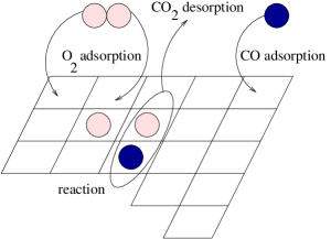
Figure 1: Reactions on a surface modelled by a two-dimensional lattice, with two types of particles, ${\rm O}$(light colored) and ${\rm CO}$(dark colored).

3. Simulations

Using different simulation techniques we want to study the evolution of the defined model over time. This means that we repeatedly execute enabled reactions on the lattice according to a simulation algorithm. There are basically two different approaches to simulate lattice models: Dynamic Monte Carlo (DMC) and Cellular Automata (CA).

Dynamic Monte Carlo

Dynamic Monte Carlo methods are used to simulate the behavior of stochastic models over time. The stochastic models of physical systems are based on a Master Equation (ME) of the form

$${dP(S,t)\over dt}=\sum_{S^{\prime}}\left[k_{SS^{\prime}}P(S^{\prime},t)-k_{S^{\prime}S}P(S,t)\right].$$ (1)

In this equation $P(S,t)$ denotes the probability to find the system in a configuration $S$ at time t, $k_{SS^{\prime}}$ is the reaction probability of the reaction that transfers $S^{\prime}$ into $S$. Such a reaction is an instance of a reaction type at a particular location.

A simulation according to this equation is essentially a discrete event simulation with continuous time, where the events are the occurences of reactions. When we assume that the rate constants do not change over time, occurrence of each event has a negative exponential distribution A.P.J.Jansen (1995); J.J.Lukkien et al. (1998). In an abstract way, a simulation then consists of a repetition of the following steps

1. Determine the list of enabled reactions.

2. Select the reaction that is the next and the time of its occurence.

3. Adjust the time and the lattice.

4. Continue from 1.

There are many different ways to organize these steps resulting in different algorithms. The taxonomy by Segers J.P.L.Segers (1999) mentions not less than 48 DMC algorithms. One of these algorithms, called the Random Selection Method (RSM) has become quite popular in the literature because of its simple implementation. It reads as follows

set time to 0;
repeat
	1. select a site $s$ randomly with probability $1/N$;
	2. select a reaction type $i$ with probability $k_{i}$/K;
	3. check if the reaction type is enabled at $s$;
	4. if it is, execute it;
	5. advance the time by drawing from
	$\left[1-\exp(-NKt)\right]$;
until simulation time has elapsed;

We denoted with $K$ the sum of the rate constants of the reaction types, i.e., $K=\sum_{i}{k_{i}}$. A single iteration of this algorithm is called a trial as no success is guaranteed. In the literature the connection with real time (step 5) is usually not mentioned. Since the method decouples the notion of time completely from the simulation (the time increment is drawn from a fixed distribution) there is a tendency to measure time in Monte Carlo steps. One MC step corresponds to one trial of a reaction type per lattice site on average, i.e., one MC step is $N$ trials.

This definition of MC steps also allows comparison between time-based simulation techniques and MC step-based techniques. Thus, one MC step is equivalent to $\sum_{j=0}^{N-1}{T_{j}},$ where the time increment $T_{j}$ is selected from the fixed distribution $1-\exp{(-NKt)}$. This value can be drawn at the end of an MC step or at the end of the entire simulation. Without using the negative exponential distribution, method RSM can also be regarded as a time discretization of the ME. The time step is then $1/NK$.

In this paper we apply method RSM because it is a DMC method that is very similar to a cellular automaton. RSM is a purely sequential algorithm that is not well suited for parallelism. In  J.P.L.Segers (1999); J.P.L.Segers et al. (1996), Segers et al. investigated how parallelism may be used in the simulation of surface reactions. The goal was to see whether simulations that are too large to run on a sequential computer may run on a parallel computer. He proposed an approach in which coherent parts of the lattice, so-called chunks, are assigned to a number of processors. The chunks are then simulated using RSM. When reactions are across multiple lattice chunks, state information has to be exchanged. Thus, synchronization and communication techniques are required for the chunk-boundaries. His investigation shows that for parallel simulations, the overhead of the parallel algorithm is considerable because of the high communication latency of parallel computers. In order to get a significant increase in speed over the sequential algorithm the amount of work on each processor must be large compared to the amount of communication. This trade-off is given by the volume/boundary ratio of the blocks. In this paper we explore another direction, viz., a parallel simulation algorithm that approximates the kinetics of the ME, thus trading accuracy for performance.

4. Cellular Automaton

Cellular Automata are a powerful tool to simulate physical and chemical systems of a high level of complexity. The CA approach is discrete in space and time. In a CA, all sites can make a reaction in each step of the simulation. For a standard Cellular Automaton the notion of real time is discarded: the decision of whether to make a reaction is based only on information local to that site. As a result, a slowly evolving reaction at some part of the lattice, has the same probability to occur as a fast reaction at another place. In order to introduce the real-time dynamics, the decision of whether to make a reaction is taken with a probability that depends on the rate constant resulting in a Non-Deterministic Cellular Automaton (NDCA). This NDCA resembles the RSM method the best. A NDCA algorithm consists of the following steps

for each step
	for each site $s$
		1.	select a reaction type $i$ with probability $k_{i}/K$;
		2.	check whether the reaction is enabled at $s$;
		3. if it is, execute it;
		4. advance the time;

In RSM and NDCA the mechanism of selecting a site is different and generates deviations in the simulation results. This happens because in a NDCA, each site is always selected during a step, while in RSM there is a non-zero probability that a site is chosen twice or more in a succesion during one simulation step. This difference in selecting a site introduces biases in the rates of the reactions and causes NDCA to give degenerate results for some systems (Ising models, Single-File models, etc.) Vichniac (1984).

The CA approach is inherently parallel and all lattice sites can be updated simultaneously in one single time step of the simulation. However, parallelism also introduces conflicts for reactions that may disable each other. Consider, for instance, a diffusion model involving two sites. A particle at site $n$ can jump to one of the neighboring sites if this is an empty site, while another particle from the same neighborhood could jump as well to the same empty site (see Fig. 2). Failure to deal with this may lead to the violation of the physical laws. We avoid erroneous simulations by adjusting the simulation model in order to avoid the conflicts that arise as a consequence of the parallel execution.

Figure 2: Conflict for simulating reactions that affect neighboring sites (such as diffusion) in a CA model. Both particle can jump to the empty site $n$ during the same step.

5. Cellular Automaton with partitions

In the literature, the problem of the conflicts in parallel simulations is solved using Block Cellular Automata (BCA). The BCA use the concept of partitioning. The sites of a CA are partitioned into a regular pattern of blocks that cover the whole space and do not overlap. A step is then applied at the same time and independently to each block. In the next step, the block boundaries are shifted such that the edges occur at a different place.

In Fig. 3 we have an example of using blocks in a very simple one-dimensional BCA. The only reaction rule is that the state of a site (0 or 1) becomes 0 if at least one of the neighboring sites is 0, otherwise it stays the same.

Figure 3: Example of a BCA where the transition is applied within blocks consisting of three sites.

To avoid the exchange of information between the blocks and the problems that might appear at the edges, we generalize this idea of a block to a partition. We define a partition $P$ as a collection $P_{i}$ of subsets of $\Omega$ called chunks, such that these chunks are disjoint and cover the entire lattice, $\Omega=\sum_{i}P_{i}$. For instance, we can write the previous example in terms of partitions. We have in this case two partitions $P$ and $Q$ consisting of three sets each where $P_{0}$=$\{$0,1,2$\}$, $P_{1}$=$\{$3,4,5$\}$, $P_{2}$=$\{$6,7,8$\}$ and $Q_{0}$=$\{$0,7,8$\}$, $Q_{1}$=$\{$1,2,3$\}$, $Q_{2}$=$\{$4,5,6$\}$.

The new definition of a partition introduces more freedom: we can assign non-adjacent sites to the chunks such that the problem with the edges between the chunks disappears. This means that the conflicts should disappear and we therefore add the following restriction.

Each site of the lattice is assigned to a chunk such that between the sites in the same chunk there are no conflicts for the given model.

This means that for all $s,t$ $\in$ $P_{i},$ $s\neq t$ and for all reaction types $Rt$, $Rt^{\prime}$

$$Nb_{Rt}(s)\cap Nb_{Rt^{\prime}}(t)=\emptyset$$

As all the sites in a chunk can be simulated simultaneously, we are interested to minimize the number of these chunks of a partition (i.e., minimize $|P|$) in order to increase parallelism.

Example

We consider again the physical model used in the previous section for $\rm CO$ oxidation on a catalyst surface (see Fig. 1). From Table 1 we can see that the reaction types do not include more than two sites. When assigning sites to the chunks we observe that a minimum number of five chunks can be used, such that the patterns of the defined reaction types applied at the sites of these chunks do not overlap. In Fig. 4 we have a block of 5 x 5 lattice sites, optimally divided into a number of five chunks. We can use this block as a pattern to tile the whole lattice.

Figure 4: The lattice is split into a number of chunks (five in this case), and the sites are distributed between these chunks. We have labelled the sites with numbers from 0 to 4, according to the chunk they belong to. The sites into one chunk can be updated simultaneously, giving a von Neumann neighborhood.

Algorithm

We give here a NDCA that uses the concept of partitions. We call it the Partitioned NDCA algorithm (PNDCA) and it reads as follows

for each step
	choose a partition $P$;
	for all $P_{i}\in P$
		for each site $s{\in}{P_{i}}$
			1.	select a reaction type with probability $k_{i}/K$;
			2.	check if the reaction is enabled at $s$;
			3.	if it is, execute it;
			4.	advance the time;

The idea is to simulate the enabled reactions according to their rate constants visiting all the sites of the chunks $P_{i}$.

Opportunities for improvements

The RSM simulations differ from PNDCA simulations for the following reasons. In a PNDCA, in a step, a site can be selected only once for the simulation because a chunk is selected once per step, and in each chunk a site is selected exactly once. After the site has been selected once, the probability to select that site again in the same step is 0. In RSM there is a probability 1/$N$ per iteration to select a site and a non-zero probability to choose the site again in the same step. Another reason is that while the reactions in a chunk are simulated, the enabled reactions in other chunks are postponed for execution.

The deviation can be made smaller through additional randomization and through re-organization of the steps in the algorithm. Depending on how the selection of a chunk is done, we can derive a set of algorithms. Chunks can be selected in the following ways:

1. all chunks in a predefined order,

2. all chunks randomly ordered,

3. a set of random chunks such that a chunk has a probability $1/|P|$ to be selected during a step,

4. a weighted selection according to the rates of enabled reactions in each chunk.

Simulating all the chunks per step in order or randomly, introduces correlations in the occupancy of the sites. More correlations between occupancy of the sites occur as less chunks are introduced. If $|P|$ is large the algorithm performs better. If $|P|=N$ and a chunk is selected randomly, PNDCA and RSM match.

We can also vary the amount of work done per chunk through the choice of the number of trials, $L$. If this number is small only a relatively small amount of time is spent within the chunk resulting in a small overall deviation. This leads to the following general structure.

for each step
	choose a partition $P$;
	set trials to 0;
	repeat
		select $P_{i}\in P~{}~{}$(probability $|P_{i}|/|P|)$;
		select $L,1\leq L\leq(N-trials)$
		set trials to trials + L;
		for $L$ sites $\in{P_{i}}$
			1.	select a reaction type with probability $k_{i}/K$;
			2.	check if the reaction is enabled at the site;
			3.	if it is, execute it;
			4.	advance the time;
	until trials = N

The number of trials per chunk is smaller than the size of a chunk, $L\leq|P_{i}|$, and the sites to be visited in a chunk are selected randomly. We name this algorithm L-PNDCA. Through special choices of the parameters that we have introduced the L-PNDCA approaches the DMC method RSM. For example, when $L$ is fixed at 1 or when $|P|$ assumes the extreme values 1 or $N$.

Another approach using partitions

The effect of the non-overlap rule is that the patterns in the model limit the choice of the partition significantly: larger patterns lead to more chunks. Since the degree of concurrency is related to the size of the chunks the non-overlap rule also limits the concurrency. By adding an additional ordering constraint we can reduce this effect as follows.

If we look at the simulation of a single chunk in the partition then this simulation proceeds by repeatedly selecting a reaction type and executing it. We re-order these steps by partitioning the set of reaction types $\cal T$ into $\sum_{j}{\cal T}_{j}$. The sets ${\cal T}_{j}$ are selected according to their rates and then the algorithm is executed for the reaction types in this selected ${\cal T}_{j}$. We can now do a partitioning of the set $\Omega$x${\cal T}$ = $\sum$ ($P_{i}$, ${\cal T}_{j}$). The non-overlap rule reduces to non-overlap with respect to the reactions types within ${\cal T}_{j}$ and, as a result, the partition can be done with fewer chunks. There is a trade-off however: the work per chunk is less, in principle.

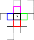
Figure 5: Overlap of the reaction patterns on the central site $s$ for the model of CO oxidation.

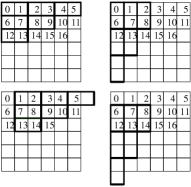
Figure 6: The four partitions of the lattice sites according to the subsets $T_{i}$ of reaction types, for the model of CO oxidation.

Example

The patterns of the reaction types that can be enabled at a specific site $s$, all contain two sites positioned as in Fig. 5 and the site $s$ can thus be a part of four possible pairs during a transformation. We split the set of reaction types in subsets, such that the patterns of the reaction types from a subset $T_{i}$ are included in only one such pair, apart from translation. The set of reaction types is then a collection of two subsets ${\cal T}_{j}$, $\cal T$=$\sum_{j=0}^{1}{{\cal T}_{j}}$ (see Table 2). The partition $P$ is a collection of only two chunks which are constructed by skipping a row or a column each time. Fig. 6 illustrates the principle for our earlier example. The chunks $P_{i}$ are the following
$P_{0}$=$\{$0, 2, 4, 7, 9, …$\}$
$P_{1}$=$\{$1, 3, 5, 6, 8, …$\}.$

$T_{0}$	$Rt_{\rm CO+O}^{(0)}$, $Rt_{\rm CO+O}^{(2)}$	$Rt_{\rm O_{2}}^{(0)}$	$Rt_{\rm CO}$
$T_{1}$	$Rt_{\rm CO+O}^{(1)}$,$Rt_{\rm CO+O}^{(3)}$	$Rt_{\rm O_{2}}^{(1)}$	-

Table 2: The new division of the reaction types in subsets ${\cal T}_{j}$, $j=0,1$ for the model in Fig. 1 applied on a site $s$.

Algorithm

The algorithm consists of the following steps

for each step
	for $|{\cal T}|$ times
		select ${\cal T}_{j}$ $\in{\cal T}$ with probability $K_{{\cal T}_{j}}/K$;
		select a reaction type from ${\cal T}_{j}$ with probability $k_{i}/k_{{\cal T}_{j}}$;
		select $P_{i}\in P$
		for each site $s{\in}{P_{i}}$
			1. check if the reaction is enabled at $s$;
			2. if it is, execute it;
			3. advance the time;

This is basically the generalization of the simulation algorithm used by Kortl$\ddot{\rm u}$ke O.Kortl$\ddot{\rm u}$ke (1998). We have used here $K_{{\cal T}_{j}}$ to denote the sum of the reaction rates of the elements from the set ${\cal T}_{j}$.

6. Correctness and performance

In order to study the correctness of our methods, we compare the kinetics of the reactions in DMC and in CA simulations. DMC is based on the following fundamental assumption known as Gillespie hypothesis:

If a reaction with a rate constant $k$ is enabled in a state $S$, then the probability of this reaction occuring in an infinitesimal time interval of size ${\delta}t$ is equal to $k{\delta}t$. The probability that more than one reaction occurs in an interval of length $\delta t$ is negligible.

The above assumption says that in any state and at any time, the probability of occurence of an enabled reaction in a vanishingly small interval is proportional to its rate, and that the probability of two reactions occuring simultaneously is negligible D.T.Gillespie (1976); Gillespie (1977); Jansen (1995). A stochastic model that respects the fundamental assumption is described by a Master Equation and can be simulated using DMC methods Kampen (1981); R.J.Gelten et al. (1999); R.J.Gelten et al. (1998a); A.P.J.Jansen (1995); R.J.Gelten et al. (1998b); J.J.Lukkien et al. (1998); K.Binder (1986).

Based on the Gillespie hypothesis, Segers et al. J.P.L.Segers (1999) has given two criteria for the correctness of the simulation algorithms of surface reactions. These criteria suggest a way to select a site and a reaction type with a correct probability. According to these criteria, each algorithm is correct if only enabled reactions are performed and 2 conditions are satisfied:

1. the waiting time for a reaction of type $i$ (the time that elapses before it occurs) has an exponential probability distribution ($\exp(-k_{i}t)$);

2. the waiting time of the next reaction type $i$ is according to the ratio between the reaction rate constant ($k_{i}$) and the sum of the rate constants of all the enabled reactions.

In our CA methods with partitions, we have seen that the order of visiting the sites is important and can introduce correlations in the simulations. Using partitions, some sites are excluded from simulation for a certain time, while others are preferred. The same problem arises for executing the enabled reactions. Executing reaction types from a chunk, disables the enabled reactions in other chunks and introduces biases in the rates of reactions. This comes from the fact that for CA methods, the fundamental assumption does not hold. In principle, many reactions can be enabled and executed during a small time interval in a CA. Thus, CA gives results that may deviate from the DMC results.

As an example for our new methods, we consider the model used by Kuzovkov et al. Kuzovkov et al. (1998) to study reactions on the surface including surface reconstruction. The model used is similar to our example model, the oxidation of CO on a face of Platinum(100). Adsorbates like CO can lift the reconstruction of the hexagonal structure of the top layer of Pt(100) to a square structure. CO adsorbs in both phases of the top layer. $\rm O_{2}$ adsorbes only in the square phase. Adsorbed CO may desorb again and O and CO may desorb associatively, forming $\rm CO_{2}$. The behavior on the surface is the following: CO adsorbs on Pt(100) in a hexagonal phase, the surface top layer reconstructs into a square structure such that $\rm O_{2}$ can now adsorb on the lattice. As $\rm O_{2}$ molecules are adsorbed, $\rm CO_{2}$ is produced and desorb liberating the lattice from particles. The surface reconstructs again to a hexagonal structure and the process is repeating: we get oscillatory behavior on the surface. We use the oscillations in the coverages with particles of the lattice for comparing our results.

Because of the absence of conflicts between the chunks, the approach with partitions leads to a significant increase in speedup even for not so large systems (100x100, 200x200). In Fig. 7 we can see how the speedup of the PNDCA algorithm depends on the system size $N$ and on the number of processors $p$. The speedup is defined as the ratio between the simulation time using 1 processor, for a system size N (T(1,N)) and the simulation time on $p$ processors, for a system size N (T($p$,N)).

Figure 7: Speedup function on the system size $N$ and on the number of processors $p$.

For the method with partitions we see that a small time spent within a chunk (small L) affects the parallelism, while a large time spent within a chunk (large L) affects the correctness.

We denote with $m$ the number of chunks ($m=|P|$). In Fig. 8 we see that for $m=1$, $L=N^{2}$ (one chunk containing all the lattice sites), and for $m=N^{2},L=1$ ($N^{2}$ chunks with one site per chunk), DMC and          L-PNDCA give the same results.

Figure 8: RSM and L-PNDCA results for the time dependence of the coverage with CO and O particles of a system of size $N$=100x100. The continous line is for RSM, and the dashed line is for L-PNDCA with parameters $m=1$, $L=N^{2}$ and $m=N^{2}$, $L=1$.

For the optimal case of five chunks, we experimented with different $L$’s. Increasing $L$ introduces biases in the simulations. In Fig. 9 we illustrate this for case $L=1$ and $L=100$, for lattice size $N$=100x100. We notice that for $L=1$, L-PNDCA gives almost the same results as DMC.

Figure 9: RSM and L-PNDCA results for five chunks and $N$=100x100. In a) $L=1$ and in b) $L$=100.

In case a chunk is selected each time with a probability $|P_{i}|/|P|$, for larger values of $L$ (e.g. $L$=100), the correlations have as effect the deviation in time of the oscillations from the DMC results. In this case, for very large values of $L$, the oscillations disappear. But, if we simulate all the chunks only once per step in a random order, we get oscillatory behavior even for very large values of $L$ ($L=N^{2}/m$)(see Fig. 10). In this case, if we consider very fast diffusion and small probabilities for chemical reactions in the cells, the deviations are so small that DMC and L-PNDCA give similar results. We can have in this case full parallelization and very accurate results.

Conclusions

We have presented a collection of approximate algorithms based on the Cellular Automaton model for parallel simulation of surface reactions. We have introduced the concept of partitions in a Non-Deterministic Cellular Automaton, and we have derived a set of parameterized algorithms based on the partitions concept. The approximation in these algorithms is introduced through parameters. The Cellular Automaton is already an approximate approach that can be taken as a starting point for simulation of surface reactions, but it gives results that deviate from the Master Equation. These CA algorithms simulate for the limit parameters the Master Equation, such that the accuracy of the simulations can be compared for different parameters sets. We find that we can get fast simulations using this approach trading accuracy for performance. We give an example when we can use full parallelization getting accurate results.

Figure 10: RSM and L-PNDCA results for five chunks ($m=5$), $N$=100x100, $L=N^{2}/m$, when all the chunks are randomly selected exactly once per step.

References

- R.J.Gelten et al. (1999) R.J.Gelten, R. Santen, and A.P.J.Jansen, Dynamic Monte Carlo simulations of oscillatory heterogeneous catalytic reactions in P.B. Balbuena and J.M.Seminario (Elsevier, Amsterdam, 1999).
- A.P.J.Jansen (1995) A.P.J.Jansen, Comput. Phys. Comm. 86, 1 (1995).
- J.J.Lukkien et al. (1998) J.J.Lukkien, J.P.L.Segers, P.A.J.Hilbers, R.J.Gelten, and A.P.J.Jansen, Phys.Rev.E 58, 2598 (1998).
- R.J.Gelten et al. (1998a) R.J.Gelten, R. Santen, and A.P.J.Jansen, Israel J.Chem. 38, 415 (1998a).
- K.Binder (1986) K.Binder, Monte Carlo methods in Statistical Physics (Springer, Berlin, 1986).
- S.V.Nedea et al. (2002) S.V.Nedea, A.P.J.Jansen, J.J.Lukkien, and P.A.J.Hilbers, Phys.Rev.E (2002).
- R.J.Gelten et al. (1998b) R.J.Gelten, A.P.J.Jansen, R. Santen, J.J.Lukkien, and P. Hilbers, J.Chem.Phys. 108(14), 5921 (1998b).
- K.M.Chandy and J.Misra (1986) K.M.Chandy and J.Misra, Communications of the ACM 24, no.11, 39 (1986).
- Fujimoto (1989) R. M. Fujimoto, Proc. 1989 International Conference on Parallel Processing III, 242 (1989).
- Reed and A.Malony (1988) D. A. Reed and A.Malony, Proc. 1988 SCS Multiconference on Distributed Simulation pp. 8–13 (1988).
- Kampen (1981) V. Kampen, Stochastic Processes in Physics and Chemistry (Elsevier Science Publishers B.V., 1981).
- C.Levermore and B.Boghosian (1989) C.Levermore and B.Boghosian, Springer Proceedings in Physics, vol. 46 (Springer, Berlin, ed. P. Manneville at al, 1989).
- Weimar (1997) J. Weimar, Simulation with Cellular Automata (Logos-Verlag, Berlin, 1997).
- Worsch (1999) T. Worsch, Future Generation Computer Systems 16, 157 (1999).
- Toffoli and Margolus (1987) Toffoli and N. Margolus, Cellular Automata Machines (Cambbridge, MA:MIT, 1987).
- R.M.Ziff et al. (1986) R.M.Ziff, E.Gulari, and Z.Barshad, Phys. Rev. Lett. 56, 2553 (1986).
- J.P.L.Segers (1999) J.P.L.Segers, Algorithms for the Simulation of Surface Processes (Ph.D. thesis, Eindhoven University of Technology, 1999).
- J.P.L.Segers et al. (1996) J.P.L.Segers, J.J.Lukkien, and P.A.J.Hilbers, High-Performance Computing and Networking. Proceedings HPCN Europe 1996 1067, 235 (1996).
- Vichniac (1984) Y. Vichniac, Physica D 10, 96 (1984).
- O.Kortlke (1998) O.Kortlke, J.Phys. A 31, 9185 (1998).
- D.T.Gillespie (1976) D.T.Gillespie, J.Comput.Phys. 22, 403 (1976).
- Gillespie (1977) D. Gillespie, J.Phys.Chem. 81, 2340 (1977).
- Jansen (1995) A. P. J. Jansen, Comput. Phys. Commun. 86, 1 (1995).
- Kuzovkov et al. (1998) V. N. Kuzovkov, O. Kortlke, and W. von Niessen, J.Chem.Phys. 108, 5571 (1998).
- B.Chopard and M.Droz (1988) B.Chopard and M.Droz, J. Phys. A 21, 205 (1988).
- B.Chopard and M.Droz (1989) B.Chopard and M.Droz, J. Stat. Phys. 64, 859 (1989).
- B.Chopard and M.Droz (1991) B.Chopard and M.Droz, Europhys.Lett. 15, 459 (1991).
- Kortlke et al. (1998) O. Kortlke, V. N. Kuzovkov, and W. von Niessen, Phys. Rev. Lett. 81, 2164 (1998).