[

Controlling the cold collision shift in high precision atomic interferometry

Abstract

We present here a new method based on a transfer of population by adiabatic passage that allows to prepare cold atomic samples with a well defined ratio of atomic density and atom number. This method is used to perform a measurement of the cold collision frequency shift in a laser cooled cesium clock at the percent level, which makes the evaluation of the cesium fountains accuracy at the $10^{-16}$ level realistic. With an improved set-up, the adiabatic passage would allow measurements of atom number-dependent phase shifts at the $10^{-3}$ level in high precision experiments.

PACS numbers: 32.88.Pj, 06.30.Ft, 34.20.Cf

]

Collisions play an important role in high precision atomic interferometry [1, 2]. In most experiments, a precise control of the atomic density is hard to achieve, which sets a limit to how accurately systematic effects due to collisions can be corrected for. This is particularly true for clocks using laser cooled Cs atoms [3, 4]. The accuracy of the BNM SYRTE cesium fountains reaches now $\sim 1\times 10^{-15}$. It is currently limited by a 10 to 20 % systematic and statistical uncertainty on the determination of the cold collision shift [5, 6, 7]. To reach such an accuracy, one has to operate with a moderate number of detected atoms, typically $10^{5}$, which sets a standard quantum limit to the frequency stability [8] of about $10^{-13}\tau^{-1/2}$, where $\tau$ is the averaging time in seconds. However, when using a high number of atoms ($10^{6}-10^{7}$), a stability approaching $3\times 10^{-14}\tau^{-1/2}$ has already been demonstrated [7, 8], which would make the evaluation at the $10^{-16}$ level practicable. Under these conditions, the cold collision frequency shift is very large ($\sim 10^{-14}$). To actually reach such an accuracy and to take full advantage of this capability, this shift has to be determined more accurately than presently achieved.

In this letter, we present a method using adiabatic passage (AP) [9, 10] that allows to prepare atomic samples with well defined density ratios. This enables the determination of the collisional frequency shift at the percent level, or better.

The measurement of the cold collision shift is based on a differential method [11]. One alternates sequences of measurements with two different, high and low effective atomic densities. One then measures the frequency difference between the two situations, as well as the difference in the number of detected atoms. Knowing the effective densities, the clock frequency can be corrected for the collisional shift by extrapolation to zero density. Unfortunately, the effective density cannot be measured directly : in a fountain, one only measures the number of detected atoms. A full numerical simulation (which takes into account the whole geometry of the fountain and the parameters of the atomic cloud) is then necessary to estimate the effective density, as in [11]. Nevertheless, extrapolating the clock frequency to zero density is still possible if one assumes that the effective density and the number of detected atoms are proportional. Under these conditions, the collisional frequency shift $\delta\nu$ is proportional to the number of detected atoms $N_{det}$, say $\delta\nu=KN_{det}$. The important point is that the coefficient $K$ should be the same for the low and high density configurations, otherwise the extrapolation to zero detected atoms is inaccurate.

Up to now, two methods have been used to change the density, and hence $N_{det}$. Atoms are initially loaded in an optical molasses, whose parameters (duration, laser intensity) can be varied. A better technique consists in keeping the same loading parameters but changing the power in a selection microwave cavity, which is used to prepare atoms in the $\left|F=3,m_{F}=0\right\rangle$ state. One can select all (resp. half) of the atoms initially in the $\left|F=4,m_{F}=0\right\rangle$ state by applying a $\pi$ (resp. $\pi/2$) pulse. However, due to the microwave field inhomogeneities in the cavity, the pulses cannot be perfectly $\pi$ and $\pi/2$ pulses for all the atoms. Both techniques affect the atomic densities, velocity distribution and collisional energy [12], and consequently the $K$ coefficients usually differ for the low and high density cases. Numerical simulations show that the $K$ coefficient may differ by 10% to 15% in our set-up, depending on parameters such as microwave power, velocity and position distribution. Fluctuations and imperfect determination of those parameters prevent from performing an accurate evaluation of the $K$ coefficient.

A method immune of these systematic effects prescribes to change the number of atoms of the sample without changing neither its velocity distribution, nor its size. This can be realized by an adiabatic transfer of population, which allows one to prepare two atomic samples, where both the ratio of the effective densities and the ratio of the atom numbers are exactly $1/2$. In contrast to previous methods, this one is insensitive to fluctuations of experimental parameters such as the size and temperature of the atomic sample, or the power coupled into the selection cavity.

First, an adiabatic passage in the selection cavity is used to transfer with a 100% efficiency all the atoms from the $\left|F=4,m_{F}=0\right\rangle$ state to the $\left|F=3,m_{F}=0\right\rangle$ state [9, 10]. This requires that the microwave field in the cavity is swept across resonance, and that the Rabi frequency $\Omega/2\pi$ has an appropriate shape and maximum intensity. We choose to use Blackman pulses (BP), following [13], which minimizes off-resonance excitation. In order to fulfill the adiabaticity condition, the frequency chirp $\delta$ has to be shaped according to

$$\delta(t)\propto\int{\Omega}^{2}(t)dt.$$ (1)

Figure 1 shows the evolution of the microwave field amplitude together with the frequency chirp.

Second, we exploit another striking property of AP. If we stop the AP sequence when $\delta=0$ (half-Blackman pulse HBP), the atoms are left in a superposition of the $\left|F=4,m_{F}=0\right\rangle$ and $\left|F=3,m_{F}=0\right\rangle$ states, with weights rigourously equal and independent of the Rabi frequency. After removal of the $\left|F=4\right\rangle$ atoms with a pushing laser beam, half of the atoms are in the $\left|F=3,m_{F}=0\right\rangle$ state, as desired.

In order to optimize this AP method and to evaluate its sensitivity to experimental parameters, we first performed a simple numerical simulation, solving the time-dependent Schr$\ddot{\rm{o}}$dinger equation for a two level atom in a homogeneous microwave field. The choice of the pulse parameters comes from a compromise between the insensitivity of the transition probabilities to fluctuations and the parasitic excitation of non-resonant transitions. Figure 2 displays as lines the calculated transition probabilities as a function of the maximum Rabi frequency $\Omega_{max}/2\pi$, for BP and HBP. The parameters were a duration $\tau_{int}=4$ ms, and $\delta_{max}=5$ kHz, which were constant over the course of the experiment. The simulation shows that the transition probabilities deviate from 1 and 1/2 by less than $10^{-3}$ as soon as $\Omega_{max}/2\pi$ is larger than 2.4 kHz. A more realistic simulation has been performed, taking into account the gaussian spatial distribution of the atomic cloud (characterized by $\sigma=3.5$ mm) in the selection cavity, its trajectory in the microwave cavity, as well as the microwave field distribution of the TE₀₁₁ mode for our cylindrical cavity. The simulation indicates that the transition probability deviates from the ideal value by less than $10^{-3}$ for both BP and HBP for all the atoms contained within $\pm 3.5\sigma$ of the vertical spatial distribution (more than 99.95 % of the atoms in the cloud). In this calculation, $\delta=0$ when the center of the cloud reaches the center of the cavity, which minimizes the sensitivity of the transfer efficiency to microwave field inhomogeneities and timing errors. For instance, a delay as large as 1 ms with respect to the optimal timing induces only a $7\times 10^{-5}$ variation on the transition probability. The only critical parameter is the accuracy of the frequency at the end of the chirp $\delta_{0}$, for HBP. We calculate a linear sensitivity of the transition probability to $\delta_{0}$ of $7\times 10^{-5}$/Hz.

We use one of our Cs fountain to demonstrate the AP method and the resulting ability to control the collisional shift. This clock is an improved version of the Rb fountain already described elsewhere [7, 14]. We use a laser slowed atomic beam to load about $10^{9}$ atoms within 800 ms in a lin $\perp$ lin optical molasses, with 6 laser beams tuned to the red of the $F=4\rightarrow F^{\prime}=5$ transition at 852 nm. The atoms are then launched upwards at $\sim 4.1$ m/s within 2 ms, and cooled down to an effective temperature of $\sim 1\mu$K. After launch, the atoms are prepared into the $\left|F=3,m_{F}=0\right\rangle$ state using a combination of microwave and laser pulses : they first enter a selection cavity ($Q\sim$1000) tuned to the $\left|F=4,m_{F}=0\right\rangle\rightarrow\left|F=3,m_{F}=0\right\rangle$ transition, where they experience either BP or HBP pulses. The atoms left in the $F=4$ state are pushed by a laser beam tuned to the $F=4\rightarrow F^{\prime}=5$ transition, 10 cm above the selection cavity. The amplitude of the pulses are shaped by applying an adequate voltage sequence (500 steps) to a microwave voltage-controlled attenuator (60 dB dynamic range), whereas the frequency chirp is performed with a voltage controlled oscillator. The Rabi frequency profile agrees with the expected Blackman shape within a few percent. The frequency chirp, and more specifically its final frequency, was not controlled as it cannot be easily checked at the required precision level of 10 Hz for HBP. The selected atoms then interact with a 9.2 GHz microwave field synthesized from a high frequency stability quartz oscillator weakly locked to the output of a H-maser. The two $\pi$/2 Ramsey interactions are separated by 500 ms. The number of atoms $N_{F=3}$ and $N_{F=4}$ are finally measured by time of flight fluorescence, induced by a pair of laser beams located below the molasses region. From the transition probabilities $N_{F=4}/(N_{F=3}+N_{F=4})$ measured on both sides of the central Ramsey fringe, an error signal is computed to lock the microwave interrogation frequency to the atomic transition using a digital servo loop.

The transition probabilities are first measured as a function of the maximum Rabi frequency $\Omega_{max}$, for the Blackman and half-Blackman pulses. The atoms are launched and selected with the pushing beam off for this evaluation phase only. To reject the fluctuations of the initial number of atoms, we measure the ratio of the atoms transferred into $\left|F=3,m_{F}=0\right\rangle$ and the total number of launched atoms, in all magnetic sub-levels. We then rescale the transfer probability in between 0 and 1 using only one free parameter : the initial population of the $\left|F=4,m_{F}=0\right\rangle$ state. The results are shown in figure 2 and reproduce very well the numerical simulations.

As the maximum Rabi frequency during the experiment was set to $7.5$ kHz, the resonance frequencies for transitions between $m_{F}\neq 0$ states have to be significantly shifted away from the 0-0 transition. A magnetic field of $\sim 180$ mG is applied during the pulses which keeps the parasitic excitation of magnetic field sensitive transitions below 0.3 %. This pulse induces a quadratic Zeeman shift on the 0-0 transition of about 14 Hz than must be taken into account to meet the resonance condition $\delta=0$ for HBP.

For each sequence of the differential measurement, we measure the mean atom number for the Blackman and half-Blackman pulses, and compute their ratio $R$. We then calculate $R_{N}$, the average of $R$ for N successive sequences. In figure 3, the standard deviation $\sigma_{R}(N)$ for various N is plotted. The stability of $R$ reaches $3\times 10^{-4}$ after a one-day integration. This reflects the insensitivity of the AP to the experimental parameter fluctuations. The mean value of the ratio is $R=0.506$, whereas it was expected to be 0.5 at the $10^{-3}$ level. This deviation cannot be explained by a non-linearity of the detection, which could arise from absorption in the detection beams. When the absorption in the detection laser beams is changed by a factor 2, we observe no change in the ratio larger than $10^{-3}$. We attribute this deviation to the uncertainty in the final frequency of the sweep. In our present set-up, the sweep is generated by an oscillator whose accuracy is limited to 50 Hz for a frequency sweep from -5 to +5 kHz (this difficulty can be solved by using a dedicated DDS numerical synthesizer). We measure a linear deviation in the transition probability of $7.5(3)\times 10^{-5}$/Hz in agreement with the predicted value. This can explain a deviation of the ratio by about $4\times 10^{-3}$. However, it is important to notice that even when the final frequency is detuned by 50 Hz, the spatial variation of the transition probability across the atomic sample is less than $10^{-3}$. All the tests performed here demonstrate that AP is at least accurate at the 1% level.

Measurements of the collisional frequency shift are then carried out using BP and HBP pulses with a large number of atoms ($N_{det}\sim 10^{7}$) in order to amplify the collisional shift. From a differential measurement, one can extrapolate the frequency of the clock at zero density with respect to the H-maser. The relative resolution of the frequency difference is $2\times 10^{-13}\tau^{-1/2}$, limited by the phase noise of the quartz oscillator used for the fountain interrogation. To check whether this extrapolation is correct, we measure the corrected frequency for two different initial temperatures of the atomic cloud, 1.1 and 2.3 $\mu$K, for which the effective densities, number of detected atoms and K coefficients are expected to be different. We switch every 50 cycles between four different configurations : 1.1 $\mu$K and BP, 1.1 $\mu$K and HBP, 2.3 $\mu$K and BP, 2.3 $\mu$K and HBP. This rejects long term fluctuations in the experiment induced by frequency drift of the H-maser used as a reference, variation of the detection responsivity, and fluctuations of other systematic effects.

The results are summarized in table I. For each configuration, the measurement of the clock frequency and number of atoms is averaged over a total time of about 50 hours. One can then extract the differential collisional shifts with a relative resolution of $5\times 10^{-16}$. The K constants are thus determined with an uncertainty of about 1 %. They are found to differ by about 20 %. The difference between the corrected frequencies can then be estimated. The uncertainty on this measurement is two-fold, a statistical uncertainty, and a systematic error which reflects the 1 % uncertainty on the ratio $R$. We find a difference between the corrected frequencies of -0.012(7)(5) mHz, which is less than 2 % of the collisional shift at high density, and compatible with zero within its error bars.

Table II displays the results obtained using either the standard selection method (SSM) or AP, for a temperature of $1.1\mu K$. The $K$ coefficients are found to differ by about 10%. Indeed, when using a $\pi/2$ pulse with the standard selection, the density distribution is transversally distorted : atoms along the symmetry axis of the cavity are more efficiently transferred than off-axis atoms. This increases the effective density for the same number of detected atoms with respect to AP, giving a larger collision shift at low density. In fact, $K$ is expected to be lower with SSM than AP, in agreement with our measurement. Extrapolating the frequency to zero density when using SSM then leads to an error of about $3\times 10^{-15}$ at this density.

It is also important to notice that we measure simultaneously the collisional frequency shift and the shift due to cavity pulling [15], which is proportional to the number of atoms crossing the Ramsey cavity. Both are correctly evaluated by our method.

In conclusion, we demonstrate here a powerful method based on an adiabatic transfer of population to prepare atomic samples with a well-defined density ratio. An important point is that the cold collisional shift is measured precisely without any absolute calibration, nor numerical simulation. This holds even when parameters of the atomic sample, or even of the atomic detection are fluctuating. This method can lead to a potential control of the cold collision shift at the $10^{-3}$ level, or even better. This capability could be demonstrated by using an ultra stable cryogenic oscillator [8], allowing a frequency resolution of $10^{-16}$ per day. Having now at hand a powerful method to determine the collisional shift with the required resolution, the evaluation of the Cs fountain accuracy at the $10^{-16}$ level is reachable. Any other high precision measurement using cold atoms should also benefit from this method to evaluate phase shifts induced by atomic interactions.

Acknowledgments: The authors wish to thank D. Calonico for his contribution in previous stage of the experiment, A. Gérard and G. Santarelli for technical assistance, and P. Lemonde for fruitful discussions. This work was supported in part by BNM and CNRS. BNM-SYRTE and Laboratoire Kastler-Brossel are Unités Associées au CNRS, UMR 8630 and 8552.

^a Present address: Time and Frequency Division National Institute of Standards and Technology 325, Broadway Boulder, Colorado 80305, USA

FIG. 1.: Temporal dependence of the Blackman pulse and the corresponding frequency chirp.

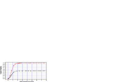
FIG. 2.: Transition probabilities for a BP and a HBP with $\tau_{int}=4$ ms, $\delta_{max}=5$ kHz as a function of $\Omega_{max}/2\pi$. The results of the numerical simulations are displayed as lines (homogeneous Rabi frequency case) and open symbols (TE011 cavity case), whereas the measurements are full symbols.

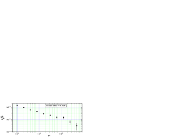
FIG. 3.: Standard deviation of the fluctuation of the ratio $R(N)$.

TABLE I.: Measurement of the cold collisional frequency shift using Adiabatic Passage. $T$ is the atomic temperature, $R$ the ratio of the number of detected atoms. The first (resp. second, when present) error bar indicated in parenthesis reflects the statistical (resp. systematic) uncertainty.

$T$	$\delta\nu$ (mHz)	$R$	$K$ ($\times 10^{-11}$) Hz/at
$1.1\mu$K	-0.323(5)	0.5063(3)	-8.62(13)
$2.3\mu$K	-0.260(5)	0.5056(3)	-10.04(20)

Difference in corrected frequency : -0.012(7)(5) mHz

TABLE II.: Comparison between the Adiabatic Passage technique (AP) and the Standard Selection Method (SSM). The temperature of the sample for these measurements was $1.1\mu$K.

	$\delta\nu$ (mHz)	$R$	$K$ ($\times 10^{-11}$) Hz/at
SSM	-0.234(7)	0.540(3)	-8.08(24)
AP	-0.275(8)	0.5054(8)	-8.97(23)

REFERENCES

- [1] C. Chin, V. Leiber, V. Vuletić, A. J. Kerman, and S. Chu, Phys. Rev. A 63, 033401 (2001)
- [2] M. Bijlsma, B. J. Verhaar, and D. J. Heinzen, Phys. Rev. A 49, R4285 (1994)
- [3] K. Gibble and S. Chu, Phys. Rev. Lett. 70, 1771 (1993)
- [4] S. Ghezali, P. Laurent, S. N. Lea, and A. Clairon, Europhys. Lett. 36, 25 (1996)
- [5] P. Lemonde et al., in Topics in Applied Physics 79, 131 (2001)
- [6] Y. Sortais et al., Physica Scripta 95, 50 (2001)
- [7] S. Bize et al., in Proceedings of 6th Symposium on Frequency Standards and Metrology (World Scientific), 53 (2001)
- [8] G. Santarelli et al., Phys. Rev. Lett. 82, 4619 (1999)
- [9] A. Messiah, Quantum Mechanics, 2, 637 (1959)
- [10] M. M. T. Loy, Phys. Rev. Lett. 32, 814 (1974)
- [11] Y. Sortais et al., Phys. Rev. Lett. 85, 3117 (2000)
- [12] P. J. Leo, P. S. Julienne, F. H. Mies, and C. J. Williams, Phys. Rev. Lett. 86, 3743 (2001)
- [13] A. Kuhn, H. Perrin, W. Hnsel and C. Salomon, in OSA TOPS on Ultracold Atoms and Bose Einstein Condensates, edited by K. Burnett (Optical Society of America, Washington, DC, 1996), Vol. 7.
- [14] S. Bize et al., Europhys. Lett. 45, 558 (1999)
- [15] S. Bize, Y. Sortais, C. Mandache, A. Clairon, and C. Salomon, IEEE Trans. on Instr. and Meas. 50, 503 (2001)