Multi-frame blind deconvolution with linear equality constraints

Abstract

The Phase Diverse Speckle (PDS) problem is formulated mathematically as Multi Frame Blind Deconvolution (MFBD) together with a set of Linear Equality Constraints (LECs) on the wavefront expansion parameters. This MFBD–LEC formulation is quite general and, in addition to PDS, it allows the same code to handle a variety of different data collection schemes specified as data, the LECs, rather than in the code. It also relieves us from having to derive new expressions for the gradient of the wavefront parameter vector for each type of data set. The idea is first presented with a simple formulation that accommodates Phase Diversity, Phase Diverse Speckle, and Shack–Hartmann wavefront sensing. Then various generalizations are discussed, that allows many other types of data sets to be handled.

Background: Unless auxiliary information is used, the Blind Deconvolution problem for a single frame is not well posed because the object and PSF information in a data frame cannot be separated. There are different ways of bringing auxiliary information to bear on the problem. MFBD uses several frames which helps somewhat, because the solutions are constrained by a requirement that the object be the same, but is often not enough to get useful results without further constraints. One class of MFBD methods constrain the solutions by requiring that the PSFs correspond to wavefronts over a certain pupil geometry, expanded in a finite basis. This is an effective approach but there is still a problem of uniqueness in that different phases can give the same PSF. Phase Diversity and the more general PDS methods are special cases of this class of MFBD, where the observations are usually arranged so that in-focus data is collected together with intentionally defocused data, where information on the object is sacrificed for more information on the aberrations. The known differences and similarities between the phases are used to get better estimates.

1 Introduction

We first present a technique for jointly estimating the common object and the aberrations in a series of images that differ only in the aberrations. With no extra information beyond the image formation model, including aberrations from the phase in the generalized pupil transmission function, it is a Maximum-Likelihood (ML) Multi-Frame Blind Deconvolution (MFBD) [(1)] method. Constraining the PSFs to be physical by requiring that they come from an underlying parameterization of the phase over the pupil is a powerful technique. Although such methods do work [(2), (3)], methods using more information work better[(4)]. Data sets used in Phase-Diverse Speckle (PDS) interferometry [(5), (6), (7)] has such extra information in the form of two (or more) imaging channels with a known difference in phase (at least to type), with Phase Diversity (PD) [(8), (9), (6)] as the special case of only one such pair (or set). These are all different data collection schemes lending themselves to similar joint inversion techniques. The purpose of the formulation presented here is to recognize the similarities and outlining a method for treating them all with a single algorithm. We discuss how the formulation accommodates also Shack–Hartmann (SH) wavefront sensing (WFS) as well as, with a couple of simple generalizations, several other types of data sets.

We start with the ML metric for a MFBD data set and derive an algorithm for the joint estimation of object(s) and aberrations for a variety of imaging scenarios. In its simplest form, it is equivalent to MFBD, while the known relations between image channels for particular data collection schemes are expressed as Linear Equality Constraints (LECs).

Throughout this paper a Gaussian noise model for the data is assumed because that permits simplifications in the ML solution methods. It is our experience with Gaussian noise PD, that it is a good model for low-contrast objects like the solar photosphere [(6)] but also that artificial high-contrast objects (like a laser–pinhole source) can often be imaged in such a way that the noise is negligible[(10)].

A code based on the formulation presented here has been successfully applied to PD, PDS, and MFBD data of various kind, both from the Swedish Vacuum Solar Telescope as well as several different simulated data sets.

2 Multi-Frame Blind Deconvolution

2.1 Forward Model and Error Metric

We use an isoplanatic image formation model with Gaussian white noise, which means that we assume that the optical system can be characterized by a generalized pupil function, which can be written, for an image frame with number $j\in\{1,\ldots,J\}$, as

$$P_{j}=A_{j}\exp\{i\phi_{j}\}$$ (1)

where $\phi_{j}$ is the phase and $A_{j}$ is a binary function that specifies the geometrical extent of the corresponding pupil. A data frame $d_{j}$ can then be expressed as the convolution of an object, $f$, and a point spread function (PSF), $s_{j}=|\operatorname{\mathfrak{F}}^{-1}\{P_{j}\}|^{2}$. In the Fourier domain we get

$$D_{j}(u)=F(u)\cdot S_{j}(u)+N_{j}(u),$$ (2)

where $S_{j}$ is the OTF, $N_{j}$ is an additive noise term with Gaussian statistics and $u$ is the 2-D spatial frequency coordinate. For brevity, we will drop this coordinate for the remainder of the paper.

We parameterize the unknown phases by expanding them in a suitable basis, $\{\psi_{m}\}$, allowing for a part of the phase, $\theta_{j}$, to be excepted from the expansion,

$$\phi_{j}=\theta_{j}+\sum_{m}^{M}\alpha_{jm}\psi_{m};\qquad\forall j.$$ (3)

The Gaussian white noise assumption allows us to use the inverse Wiener filter estimate of the object,

$$F=\frac{1}{Q}\sum_{j}S^{*}_{j}D_{j},$$ (4)

where

$$Q=\gamma_{\rm obj}+\sum_{j}^{J}|S_{j}|^{2},$$ (5)

to derive a metric in a form that does not explicitly involve the object[(8)] and that has been shown to correspond to a ML estimate of the phases[(9)]. With two regularization parameters[(11)], this metric can be written as

$$L(\mbox{\boldmath$\alpha$})=\sum_{u}\biggl{[}\sum_{j}^{J}|D_{j}|^{2}-\frac{|\sum_{j}^{J}D^{*}_{j}S_{j}|^{2}}{Q}\biggr{]}+\frac{\gamma_{\rm wf}}{2}\sum_{m}^{M}\frac{1}{\lambda_{m}}\sum_{j}^{J}|\alpha_{jm}|^{2}.$$ (6)

When minimizing $L$, the $\gamma_{\rm obj}$ term in $Q$ has the effect of establishing stability with respect to perturbations in the object. Its use in Eq. (4) suggests setting $\gamma_{\rm obj}$ to something proportional to the inverse of the signal to noise ratios of the image data frames. The other regularization parameter, $\gamma_{\rm wf}$, stabilizes the wavefront estimates and can be set by examining the relation between $L$ and the RMS of the wavefront[(12)]. For simplicity, this term is given under the assumption that the $\psi_{m}$ are Karhunen–Loève (KL)[(13)] functions, where $\lambda_{m}$ is the expected variance of mode $m$. This should work reasonably well also for low-order Zernike polynomials. In the general case, the wavefront regularization term is a matrix operation involving the covariances.[(11)]

Note that, although presented in a PD setting, this metric has nothing to do with PD per se, it is just a MFBD metric. The PD part enters in the parameterization in earlier PD methods and, equivalently, in the LECs in this presentation.

2.2 Gradient and Hessian for Traditional Phase Diversity

Efficient minimization of $L$ requires the gradients and, for some methods, the Hessian with respect to the aberration parameters. We start by considering the traditional PD problem, for which the normal equations can be written as

$${\bf A}^{\rm PD}\cdot{\delta\mbox{\boldmath$\alpha$}}-{\bf b}^{\rm PD}\simeq 0,$$ (7)

where the elements of $\alpha$ are the coefficients of an expansion of the single phase that is at the pupil of all diversity channels. The $M$ elements of ${\bf b}^{\rm PD}$ can be expressed as the Euclidean inner products, $\left\langle\cdot\,,\,\cdot\right\rangle$, of an expression for the gradient of $L$ and the aberration basis functions taken over the definition area of the basis functions,[(11)]

$$b^{\rm PD}_{m}=\left\langle-2\sum_{j=1}^{J}\operatorname{Im}\Bigl{[}P_{j}^{*}\operatorname{\mathfrak{F}}\Bigl{\{}p_{j}\operatorname{Re}\bigl{[}\operatorname{\mathfrak{F}}^{-1}\{F^{*}D_{j}-|F|^{2}S_{j}\}\bigr{]}\Bigr{\}}\Bigr{]}\,,\,\psi_{m}\right\rangle+\gamma_{\rm wf}\frac{\alpha_{m}}{\lambda_{m}}.$$ (8)

An approximation of the $M\times M$ Hessian matrix ${\bf A}^{\rm PD}$ can be derived if $Q$ is regarded as a fixed quantity[(11)]. The elements can then be written as

$$A^{\rm PD}_{m^{\prime}m}=\left\langle 4\sum_{j=1}^{J-1}\sum_{j^{\prime}=j+1}^{J}\operatorname{Im}\biggl{[}P^{*}_{j}\operatorname{\mathfrak{F}}\biggl{\{}p_{j}\operatorname{\mathfrak{F}}^{-1}\Bigl{\{}\frac{D^{*}_{j^{\prime}}}{Q}U_{jj^{\prime}}\Bigr{\}}\biggr{\}}-P^{*}_{j^{\prime}}\operatorname{\mathfrak{F}}\biggl{\{}p_{j^{\prime}}\operatorname{\mathfrak{F}}^{-1}\Bigl{\{}\frac{D^{*}_{j}}{Q}U_{j^{\prime}j}\Bigr{\}}\biggr{\}}\biggr{]}\,,\,\psi_{m}\right\rangle,$$ (9)

where

$$U_{ij}=\frac{D_{i}}{Q}\operatorname{\mathfrak{F}}\Bigl{\{}\operatorname{Im}\bigl{[}p^{*}_{j}\operatorname{\mathfrak{F}}^{-1}\{\psi_{m^{\prime}}P_{j}\}\bigr{]}\Bigr{\}}-\frac{D_{j}}{Q}\operatorname{\mathfrak{F}}\Bigl{\{}\operatorname{Im}\bigl{[}p^{*}_{i}\operatorname{\mathfrak{F}}^{-1}\{\psi_{m^{\prime}}P_{i}\}\bigr{]}\Bigr{\}}.$$ (10)

Other PD gradient and Hessian formulae are also available in the literature[(9), (6)]. We base our derivations on the ones given here, because they incorporate the regularization terms.

2.3 Gradient and Hessian for MFBD

The difference between MFBD and PD is that we in general do not know any relation between the wavefronts in the different channels. The PD gradient and Hessian expressions can then be simplified considerably by relaxing all dependencies between imaging channels, because we can then set all multiplications involving pupil quantities with different $j$ to zero. This corresponds to $J$ different pupils with independent phases.

We also have to multiply with a factor $\sqrt{J}$ for each differentiating operation. This is because we are splitting each independent variable $\alpha_{m}$ into $J$ different $\alpha_{jm}$. The vector sum of $J$ instances of identical d$\alpha_{jm}$ is $\sqrt{J}$ times larger than d$\alpha_{m}$. Because this factor appears in the denominator of the derivatives, we have to correct the gradient and the Hessian by multiplying with $\sqrt{J}$ and $J$, respectively.

We lexicographically arrange all the $\alpha_{jm}$ in a single column vector, $\alpha$, with $N=JM$ elements, so that we can also refer to them as $\alpha_{n}$, with a single index $n=(j-1)M+m$,

$$\mbox{\boldmath$\alpha$}=\begin{bmatrix}\alpha_{11}&\alpha_{12}&\dots&\alpha_{JM}\end{bmatrix}^{\rm T}=\begin{bmatrix}\alpha_{1}&\dots&\alpha_{N}\end{bmatrix}^{\rm T}.$$ (11)

We can then write the normal equations of the MFBD problem as

$${\bf A}^{\rm MFBD}\cdot{\delta\mbox{\boldmath$\alpha$}}-{\bf b}^{\rm MFBD}\simeq 0,$$ (12)

where the inner product part of Eq. (8) simplifies to the individual terms of the summations,

$$b^{\rm MFBD}_{jm}=\left\langle-2\sqrt{J}\operatorname{Im}\Bigl{[}P_{j}^{*}\operatorname{\mathfrak{F}}\bigl{\{}p_{j}\operatorname{Re}[\operatorname{\mathfrak{F}}^{-1}\{F^{*}D_{j}-|F|^{2}S_{j}\}]\bigr{\}}\Bigr{]}\,,\,\psi_{m}\right\rangle+\gamma_{\rm wf}\frac{\alpha_{jm}}{\lambda_{m}}.$$ (13)

Due to the independence between channels, the $N\times N$ Hessian ${\bf A}^{\rm MFBD}$ is block-diagonal,

$${\bf A}^{\rm MFBD}=\begin{bmatrix}{\bf A}_{1}\\ &\ddots\\ &&{\bf A}_{J}\end{bmatrix},$$ (14)

where each $M\times M$ matrix ${\bf A}_{j}$ has $A^{\rm MFBD}_{jm^{\prime}m}$ as its element at $(m^{\prime},m)$. With some arithmetics, Eq. (9) can be simplified so that these elements can be written as

$$\begin{split}A^{\rm MFBD}_{jm^{\prime}m}&=4J\left\langle\operatorname{Im}\biggl{[}\,\,\sum_{j^{\prime}=1}^{j-1}\biggl{(}P^{*}_{j^{\prime}}\operatorname{\mathfrak{F}}\biggl{\{}p_{j^{\prime}}\operatorname{\mathfrak{F}}^{-1}\biggl{\{}\frac{D^{*}_{j}}{Q}V_{j^{\prime}j}\biggr{\}}\biggr{\}}+P^{*}_{j}\operatorname{\mathfrak{F}}\biggl{\{}p_{j}\operatorname{\mathfrak{F}}^{-1}\biggl{\{}\frac{D^{*}_{j^{\prime}}}{Q}V_{j^{\prime}j}\biggr{\}}\biggr{\}}\biggr{)}+\mbox{}\right.\\ &\mbox{}\hskip 55.0pt-\left.\sum_{j^{\prime}=j+1}^{J}\biggl{(}P^{*}_{j^{\prime}}\operatorname{\mathfrak{F}}\biggl{\{}p_{j^{\prime}}\operatorname{\mathfrak{F}}^{-1}\biggl{\{}\frac{D^{*}_{j}}{Q}V_{j^{\prime}j}\biggr{\}}\biggr{\}}+P^{*}_{j}\operatorname{\mathfrak{F}}\biggl{\{}p_{j}\operatorname{\mathfrak{F}}^{-1}\biggl{\{}\frac{D^{*}_{j^{\prime}}}{Q}V_{j^{\prime}j}\biggr{\}}\biggr{\}}\biggr{)}\biggr{]}\,,\,\psi_{m}\right\rangle,\end{split}$$ (15)

where

$$V_{ij}=\frac{D_{i}}{Q}\operatorname{\mathfrak{F}}\bigl{\{}\operatorname{Im}\bigl{[}p^{*}_{j}\operatorname{\mathfrak{F}}^{-1}\{\psi_{m^{\prime}}P_{j}\}\bigr{]}\bigr{\}}.$$ (16)

3 Linear Equality Constraints

3.1 Notation and Theory

Now we add information about the data set in the form of LECs. The theory for solving optimization problems with LECs can be found in some text books on numerical methods, e.g. Ref. 14. The idea is that each constraint reduces the number of unknowns by one. We can transform a constrained optimization problem with $N$ parameters and $N_{C}$ constraints into an unconstrained problem with $N-N_{C}$ unknowns.

The constraints are given as a set of linear equations that have to be satisfied exactly,

$${\bf C}\cdot\mbox{\boldmath$\alpha$}-{\bf d}=0,$$ (17)

while minimizing $L$. With $N_{\rm C}$ linearly independent constraints, ${\bf C}$ is an $N_{\rm C}\times N$ matrix, where $N_{\rm C}<N$. This means Eq. (17) is under-determined and can therefore be solved exactly by several different $\alpha$. All solutions to Eq. (17) can be written as

$$\mbox{\boldmath$\alpha$}=\overline{\mbox{\boldmath$\alpha$}}+{\bf Q}_{2}\cdot\mbox{\boldmath$\beta$},$$ (18)

where $\overline{\mbox{\boldmath$\alpha$}}$ is a particular solution to Eq. (17) and the $N^{\prime}=N-N_{\rm C}$ column vectors of ${\bf Q}_{2}$ are an orthogonal basis of the null space of ${\bf C}$. A particular solution can always be found by setting the $N^{\prime}$ last elements of $\overline{\mbox{\boldmath$\alpha$}}$ to zero and solving the reduced system

$${\bf C}^{\prime}\overline{\mbox{\boldmath$\alpha$}}^{\prime}-{\bf d}=0,$$ (19)

where ${\bf C}^{\prime}$ is the upper left $N_{C}\times N_{C}$ submatrix of ${\bf C}$ and $\overline{\mbox{\boldmath$\alpha$}}^{\prime}$ is a vector containing the first $N_{C}$ elements of $\overline{\mbox{\boldmath$\alpha$}}$. Note, though, that all known differences can be incorporated into $\theta_{j}$, so we can set ${\bf d}\equiv 0$ without loss of generality, and we always have the particular solution $\overline{\mbox{\boldmath$\alpha$}}=0$. We can find a basis for the null space by using an orthogonal decomposition of ${\bf C}$, such as SVD or QR. With QR factorization, we write

$${\bf C}^{\rm T}={\bf Q}\cdot{\bf R};\qquad{\bf Q}=\begin{bmatrix}{\bf Q}_{1}&{\bf Q}_{2}\end{bmatrix},$$ (20)

where ${\bf Q}_{2}$ is the rightmost $N^{\prime}$ columns of ${\bf Q}$ and T used as a superscript denotes matrix transpose.

The constrained minimization problem in $\alpha$ can be transformed into an unconstrained minimization problem in a reduced set of variables, $\beta$, an $N^{\prime}$ element vector of parameters, $\beta_{n^{\prime}}$. The normal equations for the transformed problem are obtained by left-multiplying Eq. (12) with ${\bf Q}_{2}^{\rm T}$ and substituting ${\bf Q}_{2}\delta\mbox{\boldmath$\beta$}$ (Eq. (18), $\overline{\mbox{\boldmath$\alpha$}}=0$) for $\delta\mbox{\boldmath$\alpha$}$,

$${\bf Q}_{2}^{\rm T}{\bf A}^{\rm MFBD}{\bf Q}_{2}\cdot\delta\mbox{\boldmath$\beta$}-{\bf Q}_{2}^{\rm T}\cdot{\bf b}^{\rm MFBD}\simeq 0.$$ (21)

Once we have a solution for $\beta$, we easily get the solution for $\alpha$ from Eq. (18).

In order to efficiently express the LECs, we need to be able to distinguish between frames collected in different ways. We will therefore expand the $j$ index to a set of two indices, $k$ and $t$, so that $j=k+(t-1)K\in\{1,\ldots,TK\}$. We will use $k\in\{1,\ldots,K\}$ for simultaneous exposures in diversity channels and $t\in\{1,\ldots,T\}$ for discrete time or different realizations of atmospheric turbulence. With $K=1$ we have MFBD, while $T=1$ corresponds to PD. If $K=T=1$, we have the BD problem.

3.2 Phase Diversity with only Known Differences in Phase

(a) ${\bf C}^{\rm PD^{\prime}}$

(b) ${{\bf Q}}_{2}$

Figure 1: Constraints and null space matrices for PD with only known differences in phase. $K=4$ and $M=12$. White and black correspond to $\pm 1$, respectively. See Eqs. (22) and (23).

(a) ${\bf C}^{\rm PD}$

(b) ${{\bf Q}}_{2}$

Figure 2: Constraints and null space matrices for PD with two unknown phase differences, e.g. the tilts. $K=4$ and $M=12$. See Eq. (24). Compare Fig. 2.

For a PD data set ($T=1$) we know that the phases are equal, except for diversity and registration. The diversity is in $\theta_{k}$ and does not enter in the expansion in basis functions. To reduce the $KM$ wavefront parameters to $M$ unknowns, we need a constraints matrix consisting of $(K-1)M$ constraints, which can be written as

$${\bf C}^{\rm PD^{\prime}}:\quad\alpha_{1m}-\alpha_{km}=0;\qquad k>1,\quad\forall m,$$ (22)

where we momentarily disregard the registration of the imaging channels. The rows can be in any order but it seems natural to let $m$ vary faster than $k$. Using Eq. (20), we get a null space matrix. These matrices can be written in block matrix form as

$${\bf C}^{\rm PD^{\prime}}=\begin{bmatrix}{\bf I}_{M}&-{\bf I}_{M}&\\ \vdots&&\ddots&\\ {\bf I}_{M}&&&-{\bf I}_{M}\\ \end{bmatrix};\qquad{\bf Q}_{2}=\frac{1}{\sqrt{K}}\begin{bmatrix}{\bf I}_{M}\\ \vdots\\ {\bf I}_{M}\end{bmatrix},$$ (23)

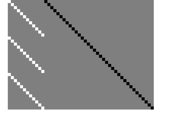
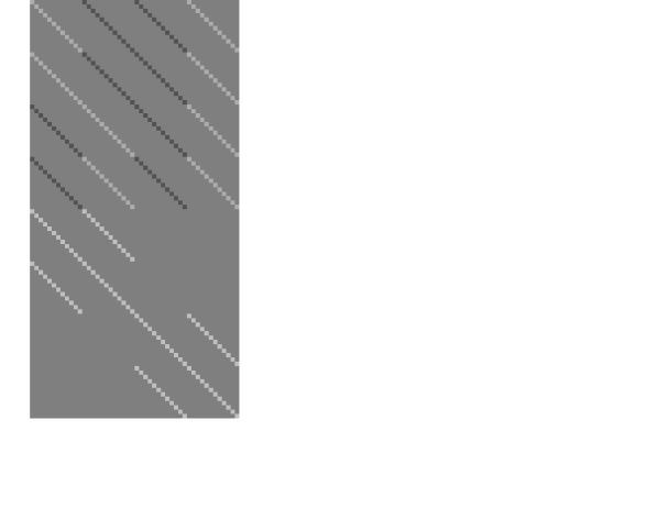
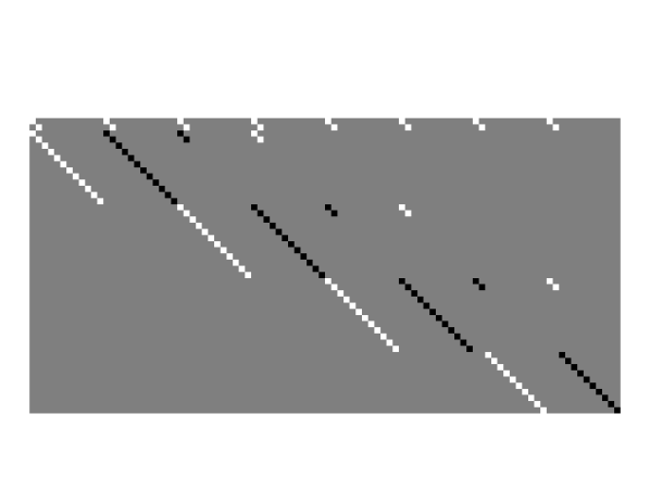
where ${\bf I}_{M}$ is the $M\times M$ identity matrix. ${\bf C}^{\rm PD^{\prime}}$ is a $(K-1)M\times KM$-matrix and the corresponding null space matrix is $KM\times M$, see example in Fig. 2. Note that this particular null space matrix (for every constraints matrix, there are infinitely many) is sparse, so matrix multiplications with ${\bf Q}_{2}$ can be fast, even for large problems.

${\bf Q}_{2}$ is easily interpreted by looking at Eq. (18). The $K$ individual $\mbox{\boldmath$\alpha$}_{j}$ are identical copies of $\mbox{\boldmath$\beta$}/\sqrt{K}$. Identical $\mbox{\boldmath$\alpha$}_{j}$ are exactly what we expect, given the constraints. Comparing Eqs. (21) and (7), it is also easy to see that ${\bf Q}_{2}^{\rm T}\cdot{\bf b}^{\rm MFBD}={\bf b}^{\rm PD}$ (except for an inconsequential constant factor in the wavefront regularization term), so the same solution minimizes the problem in either formulation. For each specific $K$ it is also easy to confirm that ${\bf Q}_{2}^{\rm T}{\bf A}^{\rm MFBD}{\bf Q}_{2}={\bf A}^{\rm PD}$. So the entire original PD problem from Sect. 2.2 is retained.

3.3 Phase Diversity with Partly Unknown Differences in Phase

For modes with unknown differences between the channels, we simply do not add any constraint, thus allowing the algorithm to optimize the corresponding coefficients independently in the two channels based on the available data. This can be used e.g. for the focus mode, if the diversity it is not known well, or for other low order modes that may differ between diversity channels.

The most common unknown differences, however, are for the tilt modes, corresponding to image registration. Unless we have information from other data sets, we generally don’t know the tilt differences. So we want to exclude the tilt modes from Eq. (22). However, we may wish to prevent a common tilt to grow without bounds by requiring that they add up to zero,

$${\bf C}^{\rm PD}:\quad\begin{cases}\sum_{k}\alpha_{km}=0;&\qquad m\in\{{\rm tilt\ modes}\}\\ \alpha_{1m}-\alpha_{km}=0;&\qquad k>1,\quad m\not\in\{{\rm tilt\ modes}\}.\end{cases}$$ (24)

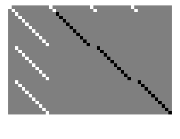
This will still allow changes in the individual tilt coefficients. A sample $((K-1)(M-2)+2)\times KM$ constraints matrix and a corresponding null space matrix are shown in Fig. 2. The modes with unknown differences (tilts) are numbered as $m\in\{1,2\}$. The null space matrix generated by my QR factorization code is not very regular but it does work, however it is not as easily interpreted as the one in the previous subsection. Also, it is not as sparse. See discussion in Sect. 5.

The number of unknowns is the $M-2$ non-tilt wavefront parameters for the common phase plus the registration of $K$ channels, which amounts to $2(K-1)$ tilt parameters. This corresponds to the total number of MFBD wavefront parameters, $KM$, minus the number of constraints, $(K-1)(M-2)+2$.

3.4 Phase Diverse Speckle

(a) ${\bf C}^{\rm PDS^{\prime}}$

(b) ${{\bf Q}}_{2}$

Figure 3: Constraints and null space matrices for PDS with only known differences in phase. $J=4$, $K=2$ and $M=12$. See Eq. (25), ignore special treatment of tilt modes.

(a) ${\bf C}^{\rm PDS}$

(b) ${{\bf Q}}_{2}$

Figure 4: Constraints and null space matrices for PDS with two unknown phase differences, e.g. the tilts. $J=4$, $K=2$ and $M=12$. See Eq. (25).

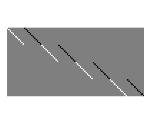
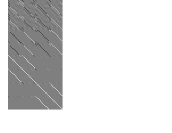
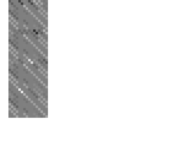
Again starting with the case of completely known phase differences, the number of wavefront parameters is $KTM$, but there are only $T$ different atmospheric realizations. The real number of unknowns is therefore $TM$ and we need $(K-1)TM$ constraints. This is $T$ times the number of constraints in the PD problem. For each $t\in\{1,\ldots,T\}$ we simply add one set of constraints of the second type in Eq. (24), see sample matrices in Fig. 4.

In practice, we must allow for unknown registration between PD channels as well as between consecutive PD sets. Normally we know that the difference in tilt between the PD channels, $k$, is constant over time, $t$. Finally, we require that the registration parameters sum up to zero independently in the two directions.

$${\bf C}^{\rm PDS}:\quad\begin{cases}\sum_{t,k}\alpha_{tkm}=0;&\qquad m\in\{{\rm tilt\ modes}\}\\ \alpha_{tkm}-\alpha_{t(k-1)m}=\alpha_{(t-1)km}-\alpha_{(t-1)(k-1)m};&\qquad t>1,\quad k>1,\quad m\in\{{\rm tilt\ modes}\}\\ \alpha_{t1m}-\alpha_{tkm}=0;&\qquad\forall t,\quad k>1,\quad m\not\in\{{\rm tilt\ modes}\}.\end{cases}$$ (25)

Note that this problem is just as constrained as the problem with completely known phase differences, thus the null space matrices have the same dimensions. See sample matrices in Fig. 4. The special tilt constraints result in a less orderly and sparse null space matrix, although not as bad as in the PD case.

When working with seeing degraded data, it is likely that all PD sets are not of the same quality. One strength with PDS is that bad data can be helped by being processed jointly with the worse data. However, intuition suggests that there are cases where the bad data disturbs the inversion of the good data. It can then be useful to calculate individual metrics for each PD set, use Eq. (6) but skip the $\gamma_{\rm wf}$ term and limit the sum over $j$ to one $t$.

$$L_{t}=\sum_{u}\biggl{[}\sum_{k}^{K}|D_{tk}|^{2}-\frac{|\sum_{k}^{K}D^{*}_{tk}S_{tk}|^{2}}{Q_{t}}\biggr{]},$$ (26)

where the sum in $Q_{t}$ is limited correspondingly. This gives good diagnostics for determining which PD sets resulted in good wavefront estimates.

3.5 Shack–Hartmann WFS

A Shack–Hartmann (SH) wavefront sensor consists of a microlens array that form a number of sub-images, each sampling different parts of the pupil. SH wavefront sensing works with point sources as well as with extended objects. An example of the latter is that it has been used with solar telescopesrimmele97high ; scharmer00workstation . A fundamental limitation for such applications is that the number of microlenses is restricted by the requirement that each sub-image must resolve solar fine structure.

Usually, the mean gradient of the phase is estimated by measuring the relative or absolute image motion in the subimages. These local tilts are then combined into a phase over the whole pupil. This means that in conventional analysis of SH wavefront data, information about wavefront curvature over the microlenses, manifested as differential blurring in the subimages, is discarded. It is only by more detailed modeling that all relevant information on the wavefronts can be extracted, which in principle should be made down to the noise level of the data.

With different $A_{j}$ for different imaging channels, $j$, Eqs. (1)–(3) accommodate SH data. The phase over the full pupil is constrained to be the same for all channels, while the different $A_{j}$ correspond to the different parts of the pupil that are sampled by the different microlenses. The constraints matrix is the same as for PD with $J$ channels.

Calibration of the relative positions of the SH sub-images is required for conventional processing. If such data are available, they can be entered as tilts in the different $\theta_{j}$. However, it should be possible to estimate these tilts from the data if $\theta_{j}$ is set to zero and local tilts are included in the parameterization of the wavefront. On the other hand, no global tilts are necessary.

It has been demonstrated in simulation with two microlenses that this image formation model allows higher modes to be estimated than with conventional local tilt approximations, because local aberrations within each subimage is taken into accountlofdahl98fast . SH data have also been considered for regular PD analysis. The microlens array acts as a single phase screen and the sub-images are regarded as a single phase diverse image, to be processed together with a conventional high-resolution imagepaxman93fine-resolution-SPIE ; schulz93estimation . Both approaches are sensitive to getting the geometry of the microlens array right (phase screen in the latter case, positions of the $A_{j}$ in the MFBD–LEC case). However, in the MFBD–LEC approach, the registration of the subimages does not have to be known; it can be estimated.

You can still use a conventional image as another image channel in the MFBD–LEC formulation. If local tilt calibration data is available, this should be straight-forward. One would want to avoid estimating local microlens tilts for the high-resolution channel. This can easily be done by adding LECs that set them to zero. See also Sect. 4.1.

4 Extending the presented formulation

The formulation presented so far was chosen so that it would be fairly straight-forward, while still accommodating PDS and SH WFS. In order to demonstrate the versatility of the LEC approach, we now discuss briefly a number of relaxations of some of the requirements, and the types of data sets that can then be treated.

4.1 Different Phase Parameterization

It is trivial to relax the requirements that $M$ is the same for every data set. The single index of the $\alpha$ and ${\bf b}$ arrays can then be written as $n=m+\sum_{j^{\prime}=1}^{j-1}M_{j^{\prime}}$ rather than $n=JM$.

One application for this is the SH processing of Sect. 3.5. If the SH sub-images are to be processed together with a conventional high-resolution image, one may want to exclude the local sub-pupil tilts from the parameterization of the phase seen by the conventional camera. See also the following subsections.

4.2 Different Objects

We can also relax the requirement that all images have the same object. This requires involving another index, say $s\in\{1,\dots,S\}$ (for “scene” or “set”), and changing the formulae for the metric and its derivatives to allow for separate objects $F_{s}$. The metric can then be written as $L=\sum_{s}L_{s}$, where $L_{s}$ is from Eq. (6) but summing over $j$ only that involves object $F_{s}$.

One application for this is high-resolution solar magnetograms, see Ref. 20; 21. Magnetograms can be made by calculating the difference between opposite polarization components of light in a Zeeman sensitive spectral line collected through a birefringent filter. Because the magnetic signal is essentially the difference between two very similar images, it is important to minimize artifacts from a number of error sources, among them registration, seeing, in particular differential seeing, and instrumental effects.

The differential seeing problem can be handled by making each image the sum of many short exposures, where bad frames are discarded and the images can be well registered before adding. The short exposures can be made simultaneously in the two polarization channels by using a polarizing beamsplitter. To reduce also the influence of different aberrations in the paths after the beamsplitter, the polarization states can be rapidly switched between the detectors, so that each polarization state is recorded with a aberrations from both paths.

In order to reduce the effects of seeing degradation of the image resolution, the two sequences of short exposures could also be MFBD restored for seeing effects. Better would be to do this using constraints that come from the fact that the aberration differences between the two channels is constant, with proper respect paid to the switching. Since registration parameters are estimated along with the phase curvature terms, this could solve the seeing problem while at the same time registering the image channels to subpixel accuracy. This should be better than registration with cross-correlation techniques, since non-symmetric instantaneous PSFs would tend to corrupt such alignment.

The fact that the differences between the two polarization signals are so subtle might inspire another approach. If the object is considered to be the same for wavefront sensing purposes, then we can treat the data as a PDS data set with zero diversity terms $\theta_{j}$. The object is the same and so are the phases, except for the registration terms.

4.3 Different wavelengths

If PDS data of the same object is collected in several different wavelengths, and the cameras are synchronized, it has been shown that wavefronts estimated from one PDS set can be used for restoration of the object seen in the data collected in the other wavelengthslofdahl01two . However, this requires information about the wavefront differences as seen by the different cameras. The differences that come from the different wavelengths can easily be calculated and other differences can be estimated from a selected subset of a larger data set and then applied to all the data under the assumption that they do not change.

This assumption could also be used to advantage in a joint treatment of the simultaneous PDS (SPDS) sets. The different-object generalization from Sect. 4.2 is used together with PDS LECs and LECs that express this assumption,

$${\bf C}^{\rm SPDS}:\quad\begin{cases}\sum_{s,t,k}\alpha_{stkm}=0;&\qquad\forall s,\quad m\in\{{\rm tilt\ modes}\}\\ \alpha_{stkm}-\alpha_{st(k-1)m}=\alpha_{s(t-1)km}-\alpha_{s(t-1)(k-1)m};&\qquad\forall s,\quad t>1,\quad k>1,\quad m\in\{{\rm tilt\ modes}\}\\ \alpha_{st1m}-\alpha_{stkm}=0;&\qquad\forall s,\quad\forall t,\quad k>1,\quad m\not\in\{{\rm tilt\ modes}\}\\ \lambda_{1}(\alpha_{111m}-\alpha_{1t1m})=\lambda_{s}(\alpha_{s11m}-\alpha_{st1m});&\qquad s>1,\quad t>1,\quad m\not\in\{{\rm tilt\ modes}\}\end{cases}$$ (27)

where $\lambda_{s}$ is the wavelength (in arbitrary units) used for set $s$. For the assumption of wavelength independent aberrations to hold, the optical system should be approximately achromatic. In practice, this means the differences between the wavelengths should not be too large.

Again, this can also be relevant for SH, if a high-resolution image is processed together with the SH data – and the wavelength is not the same in the SH sensor as in the imaging camera.

4.4 Different Numbers of Diversity Channels

Finally, we can also treat data sets with different numbers of phase diversity channels in different wavelengths. This requires a $K$ that varies with $s$, $J=\sum_{s}K_{s}$. This is perhaps most useful because it permits setting $K_{s}=1$ for some $s$. This corresponds to PDS data set in one wavelength and simultaneous MFBD data in another wavelength as in Refs. 23; 24.

We should be able to run several such sets jointly and constrain the aberration differences between different $s$ to be the same for all $t$, without requiring the object to be the same.

Again, the advantage of the joint treatment is of course that wavefront differences between different imaging cameras do not have to be calibrated but are estimated together with the aberrations that are in common to the different cameras.

5 Discussion

We have presented a formulation of the MFBD problem that accomodates the varying data collection schemes involved in PD and PDS as well as SH WFS and a number of combinations of data in different wavelengths or polarizations and with or without diversity in the phase or pupil geometry. In doing this, we have not exhausted the types of data sets that can be treated with the method presented in this paper. As long as there are known relations between the imaging channels, that can be formulated in terms of constraints on the wavefront coefficients, the data could be handled and the constraints can be used to benefit wavefront sensing and image restoration.

We have written a code that implements the method presented in this paper. It has been tested for PD, PDS and MFBD, but the other suggested processing strategies have not been tried yet. Trying some of the suggested strategies will be the subject of future papers.

The code is new and as we apply it to different problems we anticipate significant improvements in the implementation of the method as well as in the method itself. One particular area of improvement is the calculation of the null space matrix. It consists of basis vectors for the null space and for any constraints matrix, there are infinitely many null space matrices, corresponding to rotations of the coordinate system in the null space. A method for making a null space matrix that is as sparse and regular as possible would be very useful. Matrix multiplications involving sparse matrices can be performed much faster than full matrices when the size of the problem is large. Also, a null space matrix such as the one in Fig. 2 is so much more instructive and easy to interpret than the one in Fig. 2.

References

- (1) T. J. Schulz, “Multi-frame blind deconvolution of astronomical images,” Journal of the Optical Society of America A 10, pp. 1064–1073, 1993.
- (2) T. J. Schulz, B. E. Stribling, and J. J. Miller, “Multiframe blind deconvolution with real data: Imagery of the Hubble Space Telescope,” Optics Express 1(11), pp. 355–362, 1997.
- (3) W. C. Van Kampen and R. G. Paxman, “Multi-frame blind deconvolution of infinite-extent objects,” in Propagation and Imaging through the Atmosphere II, L. R. Bissonnette, ed., Proc. SPIE 3433, pp. 296–307, 1998.
- (4) D. W. Tyler, S. D. Ford, B. R. Hunt, R. G. Paxman, M. C. Roggeman, J. C. Roundtree, T. J. Schulz, K. J. Schulze, J. H. Seldin, G. G. Sheppard, B. E. Stribling, W. C. Van Kampen, and B. M. Welsh, “Comparison of image reconstruction algorithms using adaptive optics instrumentation,” in Adaptive Optical System Technologies, D. Bonaccini and R. K. Tyson, eds., Proc. SPIE 3353, pp. 160–171, 1998.
- (5) R. G. Paxman, T. J. Schulz, and J. R. Fienup, “Phase-diverse speckle interferometry,” in Signal Recovery and Synthesis IV, Technical Digest Series 11, pp. 5–7, Optical Society of America, 1992.
- (6) M. G. Löfdahl and G. B. Scharmer, “Wavefront sensing and image restoration from focused and defocused solar images,” Astronomy & Astrophysics Supplement Series 107, pp. 243–264, 1994.
- (7) R. G. Paxman, J. H. Seldin, M. G. Löfdahl, G. B. Scharmer, and C. U. Keller, “Evaluation of phase-diversity techniques for solar-image restoration,” Astrophysical Journal 466, pp. 1087–1099, 1996.
- (8) R. A. Gonsalves, “Phase retreival and diversity in adaptive optics,” Optical Engineering 21(5), pp. 829–832, 1982.
- (9) R. G. Paxman, T. J. Schulz, and J. R. Fienup, “Joint estimation of object and aberrations by using phase diversity,” Journal of the Optical Society of America A 9(7), pp. 1072–1085, 1992.
- (10) M. G. Löfdahl, G. B. Scharmer, and W. Wei, “Calibration of a deformable mirror and Strehl ratio measurements by use of phase diversity,” Applied Optics 39(1), pp. 94–103, 2000.
- (11) C. R. Vogel, T. F. Chan, and R. J. Plemmons, “Fast algorithms for phase diversity-based blind deconvolution,” in Adaptive Optical System Technologies, D. Bonaccini and R. K. Tyson, eds., Proc. SPIE 3353, 1998.
- (12) H. W. Engl, M. Hanke, and A. Neubauer, Regularization of Inverse Problems, vol. 375 of Mathematics and Its Applications, Kluwer Academic Publishers, Dordrecht, Netherlands, 1996.
- (13) N. Roddier, “Atmospheric wavefront simulation using Zernike polynomials,” Optical Engineering 29(10), pp. 1174–1180, 1990.
- (14) D. Kahaner, C. Moler, and S. Nash, Numerical Methods and Software, Prentice Hall, 1989.
- (15) T. Rimmele, J. M. Beckers, R. B. Dunn, R. R. Radick, and M. Roeser, “High resolution solar observations from the ground,” in The High Resolution Solar Atmospheric Dynamics Workshop, PAPSP conference series, 1997.
- (16) G. B. Scharmer, M. Shand, M. G. Löfdahl, P. M. Dettori, and W. Wei, “A workstation based solar/stellar adaptive optics system,” in Adaptive Optical Systems Technologies, P. L. Wizinowich, ed., Proc. SPIE 4007, pp. 239–250, 2000.
- (17) M. G. Löfdahl, A. L. Duncan, and G. B. Scharmer, “Fast phase diversity wavefront sensing for mirror control,” in Adaptive Optical System Technologies, D. Bonaccini and R. K. Tyson, eds., Proc. SPIE 3353, pp. 952–963, 1998.
- (18) R. G. Paxman and J. H. Seldin, “Fine-resolution astronomical imaging with phase-diverse speckle,” in Digital Recovery and Synthesis II, P. S. Idell, ed., Proc. SPIE 2029, pp. 287–298, 1993.
- (19) T. J. Schulz, “Estimation-theoretic approach to the deconvolution of atmospherically degraded images with wavefront sensor measurements,” in Digital Recovery and Synthesis II, P. S. Idell, ed., Proc. SPIE 2029-31, 1993.
- (20) H. Lundstedt, A. Johannesson, G. Scharmer, J. O. Stenflo, U. Kusoffsky, and B. Larsson, “Magnetograph observations with the Swedish solar telescope on La Palma,” Solar Physics 132, pp. 233–245, 1991.
- (21) B. W. Lites in Solar Polarimetry, L. J. November, ed., Proc. 11th Sacramento Peak Summer Workshop, p. 173, 1991.
- (22) M. G. Löfdahl, T. E. Berger, and J. H. Seldin, “Two dual-wavelength sequences of high-resolution solar photospheric images captured over several hours and restored by use of phase diversity,” Astronomy & Astrophysics 377, pp. 1128–1135, 2001.
- (23) R. G. Paxman and J. H. Seldin, “Phase-diversity data sets and processing strategies,” in High Resolution Solar Physics: Theory, Observations and Techniques, T. Rimmele, R. R. Radick, and K. S. Balasubramaniam, eds., Proc. 19th Sacramento Peak Summer Workshop, ASP Conf. Series vol. 183, pp. 311–319, 1999.
- (24) A. Tritschler and W. Schmidt, “Sunspot photometry with phase diversity. I. Methods and global sunspot parameters,” Astronomy & Astrophysics 382, pp. 1093–1105, 2002.