Mechanism of finite-amplitude double-component convection due to different boundary conditions

Abstract

A new mechanism of double-component convection is discovered. It emerges in a horizontal layer of Boussinesq fluid as a stable stratification due to flux boundary conditions is added to an unstable gradient specified by fixed boundary values. Driven by this mechanism, steady finite-amplitude flows reminiscent of Rayleigh—Benard convection arise even when the background density stratification is stable.

1 Introduction

Double-component convection is relevant to as diverse fields as small-scale oceanography [1], astrophysics [2], geodynamo [3], crystal growth [4], colloidal suspensions [5], and soap films [6]. Convective flows are also commonly used for testing the ideas related to transition to turbulence and nonlinear pattern formation [7, 8]. In addition, double-component flows where a distinction between the components comes from component different boundary conditions are of basic significance for large-scale environmental phenomena. These phenomena range from Langmuir circulations [9] to the global ocean thermohaline circulation and climate change [10, 11].

One major aspect of double-component flows with different boundary conditions is that the effect of such conditions can be conceptually analogous to that of different diffusivities in conventional double-diffusive convection [12, 13, 14]. In particular, unequal diffusion gradients forming in perturbed state due to different boundary conditions trigger convection analogously to the classical double-diffusion. Such analogy has been introduced in [15, 16, 17, 18] as a result of the generalization of an earlier idea highlighted in [19].

This work reports the existence of a novel mechanism of double-component convection. The nature of this mechanism stems from different boundary conditions but is not underlain by the differential diffusion caused by unequal perturbation gradients of the components (differential gradient diffusion). This mechanism has been identified in a horizontal layer of pure, Boussinesq fluid where an unstable gradient of the component whose boundary values are fixed is combined with a stable stratification due to the flux boundary conditions for another component. It manifests itself in the form of finite-amplitude steady flows before the onset of the respective linear instability. Not resulting from differential diffusion, such flows arise even when the net background stratification is stable. An appropriate perturbation could thus trigger convection in a broad range of parameters where such convection could not have been previously anticipated.

2 The problem formulation and solution procedures

Let the diffusivities of the components be equal and let a stable stratification due to the component with flux boundary conditions be combined with an unstable gradient of the component with the fixed-value conditions. The diffusivities are set equal to eliminate the effects of the classical double-diffusion, and thus to examine the effects of different boundary conditions separately. This is analogous to the approach used in previous studies of conventional double-diffusive convection. In most such studies, the components with unequal diffusivities have not been distinguished from each other in terms of boundary conditions. Equal diffusivities could, besides, characterize two solutes, as claimed in [20]. The ratio of the viscosity to diffusivity (which is the Prandtl number, $Pr$) would then be different from that for temperature in water ($Pr=6.7$) used in this work. This parameter, however, is not expected to have a qualitative effect on the novel phenomenon reported herein. Equal diffusivities could also be viewed as eddy coefficients [9, 11], when the ratio between the viscosity and diffusivity is close to its value used below.

The background gradients are represented by the Rayleigh numbers $Ra=g\alpha|\Delta\overline{T}|d^{3}/\kappa\nu$ and $Ra^{s}=g\beta|\partial\overline{S}/\partial\overline{x}|d^{4}/\kappa\nu\equiv\mu Ra$. Here, $\overline{x}$ is the (dimensional) vertical coordinate, $d$ is the width of the horizontal slot, $\Delta\overline{T}$ is the (dimensional) difference between the values of temperature (standing for the component with fixed-value boundary conditions) at the lower and upper boundaries, $\partial\overline{S}/\partial\overline{x}$ is the boundaries-prescribed (dimensional) vertical derivative of solute concentration (standing for the component with flux boundary conditions), $\alpha$ is the coefficient of thermal expansion, $\beta$ is the coefficient of the density variation due to the variation of solute concentration, $g$ is the gravitational acceleration, $\nu$ is the kinematic viscosity, and $\kappa=\kappa_{T}=\kappa_{S}$ is the diffusivity of both components. The bar means that the respective variable is dimensional.

The configuration just described is illustrated in Fig. 1 as $\theta=0$, $\theta$($>0$ in Fig. 1) is the angle between the direction opposite to the gravity and that of the across-slot coordinate axis. With $\Delta_{L}\equiv\partial^{2}/\partial x^{2}+\partial^{2}/\partial y^{2}$, $\partial_{\tau}\equiv\partial/\partial\tau$, $\partial_{x}\equiv\partial/\partial x$, and $\partial_{y}\equiv\partial/\partial y$, the equations describing the two-dimensional problem in Fig. 1 in terms of streamfunction $\psi$, $t$, and $S$ are:

$$Pr(\partial_{\tau}+\partial_{x}\psi\partial_{y}-\partial_{y}\psi\partial_{x})\Delta_{L}\psi=$$

$$(\partial_{x}t-\partial_{x}S)sin\theta-(\partial_{y}t-\partial_{y}S)cos\theta+Pr\Delta_{L}^{2}\psi,$$ (1)

$$Pr(\partial_{\tau}+\partial_{x}\psi\partial_{y}-\partial_{y}\psi\partial_{x})\xi_{i}=\Delta_{L}\xi_{i},\hskip 28.45274pti=1,2.$$ (2)

Here $\xi_{1}$ and $\xi_{2}$ stand for $t$ and $S$, the across-slot velocity $u=-\partial_{y}\psi$, the along-slot velocity $v=\partial_{x}\psi$, and $\tau$ is the time. This problem was studied for $\theta=0$ and the periodic boundary conditions with period $\lambda=\overline{\lambda}/d=2$ in the along-slot direction by continuation [21] of (finite-difference) steady solutions in $Ra$ and $\mu$, the numerical approach was the same as in [15, 17, 18]. For clarification of one relevant issue arising for $\theta>0$ (this case will be explicitly identified below), continuation in $\theta$ was also used. $S=0$ was set at the middle points of the across-slot boundaries, along with the otherwise periodic conditions. Such a condition is needed to specify the scale of $S$ and the phase of a nontrivial steady solution. The time evolution of a linear perturbation initially imposed on the steady flows was computed to examine the solution stability. The stability of the conduction base flow to steady disturbances was also analyzed for different wave numbers $k=2\pi/\lambda$. This was done by searching for the smallest-$Ra$ singularity of the matrix resulting from the application of boundary conditions to the general solution of the steady, marginal linear stability problem.

3 Background

An infinitesimal disturbance imposed on the conduction state (Fig. 1, $\theta=0$) would lead to the formation of unequal perturbation gradients. Due to the differential gradient diffusion in perturbed state, a rising (sinking) fluid element would experience the buoyancy force directed downwards (upwards) [19]. The buoyancy force is thus expected to act against the sense of rotation of a small-amplitude perturbation cell. This permits amplitude growth of the perturbation cells changing their sense of rotation with adequate frequency, as illustrated in [19] for the inviscid fluid. (As highlighted in [15, 16], this effect makes the present configuration, as well as the configuration in [19], analogous to the diffusive regime of conventional double-diffusive convection [12, 13].) Such oscillatory instability also arises in the viscous fluid (Fig. 2), when the stable flux stratification increases. A detailed discussion of the effect of viscosity on manifestation of the oscillatory instability on different scales is beyond the scope of this work. Its main idea is given in [22].

(In the framework of current discussion, an oscillatory perturbation could be viewed as a standing wave, i.e., as the convective cells whose sense of rotation changes periodically in time. The prescribed across-slot-boundary values of $S$ can prevent traveling-wave disturbances from being detected in the present formulation. However, traveling waves are also expected to arise from such Hopf bifurcations as H in Fig. 2 if the translation symmetry of the conduction state is allowed for [23]. Their presence, in particular, may affect the stability of steady branches in Fig. 2.)

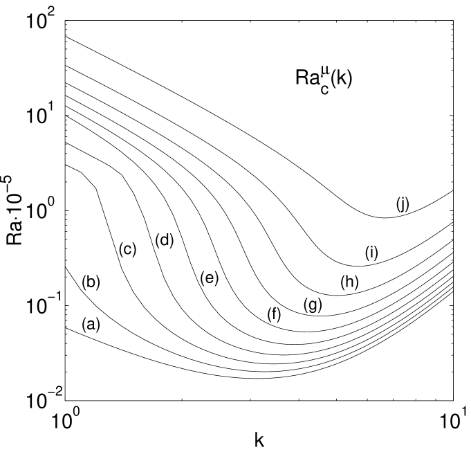
Since the differential (gradient) diffusion in the perturbed state (Fig. 1, $\theta=0$) results in the growth of oscillatory infinitesimal disturbances, it is expected to oppose growth of the small stationary perturbations. (The sense of rotation of a stationary-perturbation cell does not change. The cell amplitude could thus grow only against the above effect of differential gradient diffusion.) Indeed, $Ra_{c}^{\mu}(k)$ in Fig. 3 increasingly exceeds $Ra_{c}^{0}(k)/(1-\mu)$ as $\mu$ grows from $0$. [$Ra_{c}^{0}(k)/(1-\mu)$ are the values $Ra_{c}^{\mu}(k)$ would take on if both boundary conditions were of the fixed-value type.] The deviation of $Ra_{c}^{\mu}(k)$ in Fig. 3 from $Ra_{c}^{0}(k)/(1-\mu)$ is particularly pronounced for the large scales (small $k$), where diffusion is most effective. With respect to infinitesimal steady disturbances, therefore, flux boundary conditions for the solute stratification stabilize the conduction state compared to the single-component problem with the unstable fixed-value gradient.

4 Results and discussion

The basic result of this work is that a novel physical mechanism due to different boundary conditions (Fig. 1, $\theta=0$) gives rise to finite-amplitude convective steady flows where the conduction state is stable to the infinitesimal steady disturbances (Fig. 2). As in convection resulting from differential gradient diffusion, one element of this mechanism is disparate responses of the component stratifications to convective motion. In the present mechanism, however, the feedback to convective perturbation arises from finite-amplitude Rayleigh—Benard convection. This is essentially different from differential gradient diffusion in [15, 16, 17, 18, 19]. With such new feedback, different boundary conditions are found to result in a purely nonlinear manifestation of convection being due to the statically stable net vertical stratification.

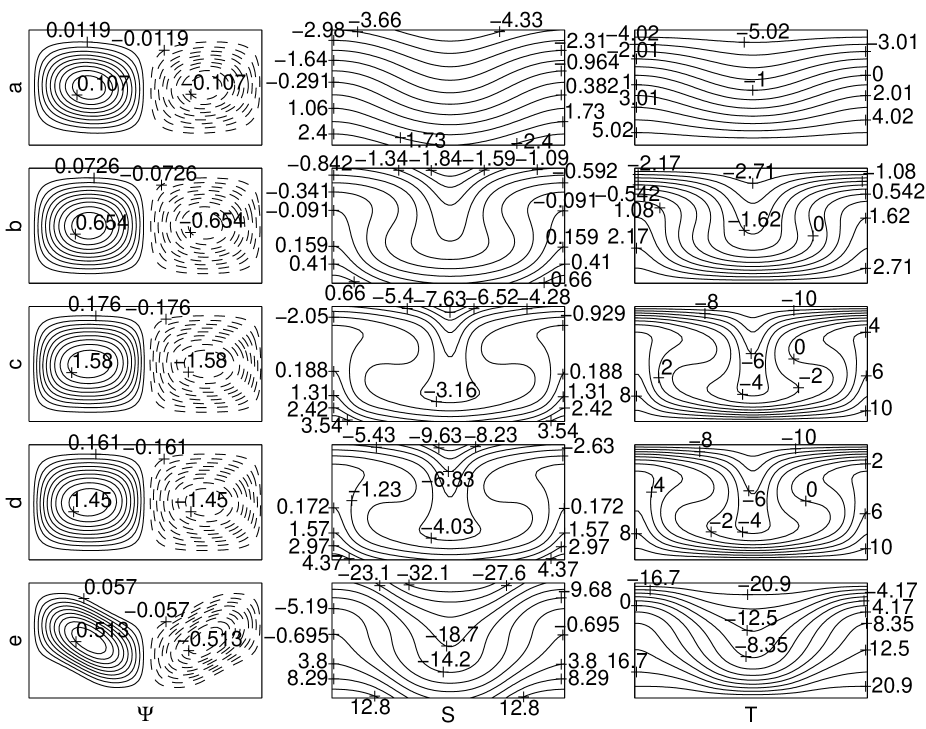
Finite-amplitude convective flows are illustrated in Fig. 4. As the convection amplitude increases [Fig. 4(a),(b)], the ratio of the across-slot solute concentration scale to such scale in the background state decreases. This is the result of an increasing number of solute isolines moving ”outside” the flow domain, especially in the regions of across-slot motion. Such behavior is associated with the flux conditions permitting solute isolines to cross the boundaries. The respective ratio for the temperature, however, remains equal to one, even when convection becomes well-developed [Fig. 4(c),(d)]. The fixed-value boundary conditions maintain the vertical temperature scale by preventing the intersection of isotherms with the boundaries. They also increase the thermal gradient near the wall towards which the across-slot component of convection is directed.

The unstable density gradients thus formed in the regions of across-slot motion in Fig. 4 substantially exceed $Ra_{c}^{0}(\pi)$ in Fig. 3(a). [$Ra_{c}^{0}(k)$ in Fig. 3(a) represents the onset of Rayleigh—Benard convection.] Such gradients result in a horizontal density difference between two streamline points, as in Rayleigh—Benard convection. This gives rise to (positive) convective feedback that maintains the disparity between component gradients. Such feedback forms even when the net background stratification is neutral or stable [Fig. 4(c),(d)]. In such cases of the present formulation, linear steady instability does not arise, as in the scenario first proposed in [24]. As $\mu$ increases, the cells at the smaller-amplitude branch, $A1$, change their form to utilize the regions with maximal gradient disparity more efficiently [Fig. 4(e)].

The analogy in the physics of oscillatory instability between the present configuration and the diffusive regime of conventional double-diffusive convection [13] does not seem to apply to finite-amplitude steady instability in both these problems. The finite-amplitude mechanism in [13] hinges on the disparity between component diffusivities. Such a disparity makes the unstable temperature gradient relatively insensitive to a convective perturbation. This gives rise to the feedback maintaining convection. In the present mechanism, differential gradient diffusion plays only a stabilizing role as the (feedback) unstable density stratification arises from the interaction of perturbation with boundary conditions. In contrast to [13], in particular, subcritical steady convection arises in the present problem even when the density stratification is statically stable.

Nonlinear Rayleigh—Benard convection also gives rise to feedback in the finite-amplitude steady instability in binary fluid [25], if the separation ratio is negative. However, the binary-fluid finite-amplitude mechanism is underlain by the dependent nature of the stabilizing background (Soret) solute gradient, rather than by boundary conditions. Such solute gradient is thus largely destroyed when its conduction-state relation to the unstable temperature gradient is relaxed by a finite convective perturbation.

Let $\theta>0$ in Fig. 1 and let $\mu=1$. When $\theta=\pi/2$, finite-amplitude steady flows arise due to differential gradient diffusion [18]. For large enough convection amplitudes ($Ra\geq\sim 20000$), the dissimilarity between the nature of such flows at $\theta=\pi/2$ and that of finite-amplitude steady convection at $\theta=0$ was found to give rise to a region of hysteresis in $\theta$. Within this region, different convective steady flows with $\lambda=2$ coexist. One of these solutions was continued from $\theta=\pi/2$ in decreasing $\theta$. For say $Ra=31000$, it extends to $\theta\approx 0.38\pi/2$. Another such flow was continued from $\theta=0$ in increasing $\theta$. For $Ra=31000$, it extends to $\theta\approx 0.51\pi/2$. For the same $Ra$($\approx 31000$), such hysteresis phenomenon was not found between $\theta=\pi/2$ and $\theta=\pi$, where steady convection is driven only by differential gradient diffusion [15, 16, 18]. A detailed analysis of the flow transformations will be reported separately.

5 Conclusions

Underlying a fundamentally new convective mechanism, different boundary conditions thus result in finite-amplitude steady convection arising in a horizontal layer of pure fluid well before the respective linear instability. Such nonlinear convective flows also exist when the vertical density stratification is statically stable. The new mechanism has to remain basically relevant for $Le\neq 1$, as well as under different $Pr$ (as say for two solutes) and stress-free boundaries, among other changes. It also raises the issue of three-dimensional effects. Another issue is the existence of an analogous effect (as well as of the effects of differential gradient diffusion) when the buoyancy forces are replaced by the forces due to surface tension. All this leads to a new perspective on the role of convection and different boundary conditions in double-component fluid systems, including the large-scale systems relevant to global environmental processes.

Figure 1: The problem in a horizontal ($\theta=0$) and inclined ($\theta>0$) slot. $\delta\rho=\rho-\rho_{0}$ is the variation of the (dimensionless) density, $\rho$, due to the variations $\delta S$ and $\delta T$ of solute concentration $S$ and temperature $T=(T_{1}+T_{2})/2+t$ with respect to their reference values, at which the density is $\rho_{0}$; $T_{1}$ and $T_{2}$ are the boundary temperatures, $\sigma=gd^{3}/\kappa\nu$. $Pr\equiv\nu/\kappa=6.7$, $Le\equiv\kappa_{T}/\kappa_{S}=1$; $\kappa_{T}$ and $\kappa_{S}$ ($=\kappa$) are the component diffusivities. The fluid is of the Boussinesq type.

Figure 2: $\theta=0$. Schematic structures of the steady flows with minimal period $\lambda=2$ for $\mu\in[0,1.2]$ ($Pr=6.7$, $Le=1$). $\Phi$ is an abstract measure of the steady flows that distinguishes between different steady solutions, specifies the location of the singularities (limit points and bifurcation points), and represents the flows arising from a symmetry-breaking bifurcation as a single branch. The background states are depicted by the horizontal lines with arrows (for $\mu=1.2$, this is the coordinate axis). The solid lines stand for the stable solutions. The dashed lines represent the flows being unstable to either steady or both steady and oscillatory disturbances. The dotted lines stand for the solutions being unstable to oscillatory disturbances alone. [Instability of the background state to steady disturbances with wave number $k=2\pi$ ($\lambda=1$), arising before that with $k=\pi$ ($\lambda=2$) at $\mu=0.6$, is not shown.] $B$ is the bifurcation standing for the steady linear stability boundary for wave number $k=\pi$ ($\lambda=2$); it changes its criticality at $\mu$ just below $0.2$ and moves to infinite $Ra$ as $\mu\rightarrow 1$. $L$ is the limit point standing for the finite-amplitude steady stability boundary for the flows with minimal period $\lambda=2$. It moves to $Ra\approx 25772$ as $\mu$ increases to $1.5$. $A1$ and $A2$ are the unstable and stable (to steady disturbances) branches associated with the limit point, respectively. H is a Hopf bifurcation. For $\mu=1$, it arises at $Ra\approx 29000$.

Figure 3: $\theta=0$. Curves of marginal linear stability to steady disturbances for different $\mu$ ($Le=1$), $Ra_{c}^{\mu}(k)$. (a) $\mu=0$; (b) $\mu=0.1$; (c) $\mu=0.2$; (d) $\mu=0.3$; (e) $\mu=0.4$; (f) $\mu=0.5$; (g) $\mu=0.6$; (h) $\mu=0.7$; (i) $\mu=0.8$; (j) $\mu=0.9$.

Figure 4: $\theta=0$. Convective steady flows ($Pr=6.7$, $Le=1$); $\lambda=2$. $\Psi$: streamlines; $S$: isolines of solute concentration; $T$: isotherms ($t$ in Fig. 1). The solid and dashed streamlines represent the clockwise and counterclockwise rotation, respectively. The actual values of $S$ and $t$ are equal to $10^{3}$ times the respective values in the figure. (a) $\mu=0.6$, $Ra=12046$, branch $A1$ (directly unstable); (b) $\mu=0.6$, $Ra=6500$, branch $A2$; (c) $\mu=1$, $Ra=24000$, branch $A2$; (d) $\mu=1.2$, $Ra=24000$, branch $A2$; (e) $\mu=1.2$, $Ra=50090$, branch $A1$ (directly unstable).

References

- [1] R. W. Schmitt, Annu. Rev. Fluid Mech. 26 (1994) 255.
- [2] E. A. Spiegel, Annu. Rev. Astron. Astrophys. 10 (1972) 261; D. W. Hughes, M. R. E. Proctor, Annu. Rev. Fluid Mech. 20 (1988) 187; V. M. Canuto, Astrophys. J. 524 (1999) 311.
- [3] F. H. Busse, Geophys. Res. Lett. 29 (2002) 1105.
- [4] S. R. Coriell, R. F. Sekerka, PCH PhysicoChem. Hydrodyn. 2 (1981) 281.
- [5] D. M. Mueth, J. C. Crocker, S. E. Esipov, D. G. Grier, Phys. Rev. Lett. 77 (1996) 578.
- [6] B. Martin, X. L. Wu, Phys. Rev. Lett. 80 (1998) 1892.
- [7] R. P. Behringer, Rev. Mod. Phys. 57 (1985) 657.
- [8] M. C. Cross, P. C. Hohenberg, Rev. Mod. Phys. 65 (1993) 851; E. Bodenschatz, W. Pesch, G. Ahlers, Annu. Rev. Fluid Mech. 32 (2000) 709.
- [9] S. Leibovich, Annu. Rev. Fluid Mech. 15 (1983) 391.
- [10] H. Stommel, Tellus 13 (1961) 224; G. Walin, Palaeogeogr. Palaeoclimatol. Palaeoecol. 50 (1985) 323.
- [11] H. A. Dijkstra, M. J. Molemaker, J. Fluid Mech. 331 (1997) 169; see also the references therein.
- [12] M. E. Stern, Tellus 12 (1960) 172.
- [13] G. Veronis, J. Mar. Res. 23 (1965) 1; J. Fluid Mech. 34 (1968) 315; R. L. Sani, AIChE (Am. Inst. Chem. Eng.) J. 11 (1965) 971.
- [14] M. E. Stern, Deep-Sea Res. 14 (1967) 747.
- [15] N. Tsitverblit, in: S. Meacham (Ed.), Double-Diffusive Processes, Woods Hole Oceanographic Institution, Technical Report No. WHOI-97-10, 1997, pp. 145-159.
- [16] N. Tsitverblit, Phys. Fluids 9 (1997) 2458.
- [17] N. Tsitverblit, Phys. Fluids 11 (1999) 2516.
- [18] N. Tsitverblit, Phys. Rev. E 62 (2000) R7591.
- [19] P. Welander, Tellus 41A (1989) 66.
- [20] A. A. Predtechensky, W. D. McCormick, J. B. Swift, Z. Noszticzius, H. L. Swinney, Phys. Rev. Lett. 72 (1994) 218; A. A. Predtechensky, W. D. McCormick, J. B. Swift, A. G. Rossberg, H. L. Swinney, Phys. Fluids 6 (1994) 3923.
- [21] H. B. Keller, in: P. H. Rabinowitz (Ed.), Applications of Bifurcation Theory, Academic, New York, 1977, pp. 359-384.
-
[22]
N. Tsitverblit,
Geophys. Res. Abs. 4 (2002) CD-ROM; see also
http://www.copernicus.org/EGS/egsga/nice02/programme/overview.htm. - [23] J. D. Crawford, E. Knobloch, Annu. Rev. Fluid Mech. 23 (1991) 341.
- [24] S. Rosenblat, S. H. Davis, SIAM (Soc. Ind. Appl. Math.) J. Appl. Math. 37 (1979) 1.
- [25] W. Barten, M. Lücke, M. Kamps, R. Schmitz, Phys. Rev. E 51 (1995) 5636.