Reaction-diffusion dynamics: confrontation between theory and experiment in a microfluidic reactor

Abstract

We confront, quantitatively, the theoretical description of the reaction-diffusion of a second order reaction to experiment. The reaction at work is $\text{Ca}^{2+}$/CaGreen, and the reactor is a T-shaped microchannel, 10 $\mu$m deep, 200 $\mu$m wide, and 2 cm long. The experimental measurements are compared with the two-dimensional numerical simulation of the reaction-diffusion equations. We find good agreement between theory and experiment. From this study, one may propose a method of measurement of various quantities, such as the kinetic rate of the reaction, in conditions yet inaccessible to conventional methods.

Chemical reaction processes taking place in spatially extended reactors with no active mixing are described by reaction-diffusion equations. In general, these equations are non linear and they possess a rich variety of solutions, giving rise to many different spatio-temporal patterns. Reaction-diffusion equations have been known for more than a century but the first elementary solutions were calculated much more recently by Gálfi and Rácz Gálfi and Rácz (1988). Their analytical solutions were obtained for a reaction of second order in an infinite domain with stepwise initial conditions, in the asymptotic limit of long times. Under these conditions, exact scaling laws were derived showing, for instance, that the position of the maximum of the production rate grows as $t^{1/2}$ while the width of the reaction production zone grows as $t^{1/6}$. Furthermore, the approach to the asymptotic state was studied by Taitelbaum et al. Taitelbaum et al. (1992) and they observed a slow approach to the asymptotic state, which was modeled by using perturbation analysis and could not be described by the long time asymptotics.

At the experimental level, one is often confronted with the additional presence of advection in the fluid. For this reason, reactions are often studied in small capillary tubes where no large scale flow is present. Such systems have been used Koo and Kopelman (1991); Park et al. (2001) to study a reaction process with initially separated reactants, validating the power law predictions of Gálfi and Rácz at asymptotically long times. Furthermore, recent experiments in porous media Léger et al. (1999) have shown very good agreement between theory and experiment in the asymptotic regime, in the case of one diffusing reactant into a solid substrate.

Here, we address the more general problem of two diffusing, initially separated, reactants in a regime that spans both the initial transients and the asymptotic state. In contrast with previously published work Koo and Kopelman (1991); Léger et al. (1999), we turn our attention to the reaction product and its concentration, instead of the production rate. This analysis takes into account the diffusion of the product as well as the reagents. We compare numerical and experimental measures of the reaction region, beyond the scaling of the different quantities, to study the shape of the concentration profiles.

Microfluidic circuits are used to achieve low Reynolds numbers ($Re\simeq 1$), thus removing any effects of advection without resorting to gels or other media. We believe that the detailed comparison of the shape of the concentration profiles between simulations and experiments allows one to assess to what extent, from the dynamical viewpoint, modeling a reaction by a kinetics of a prescribed order is accurate. This assessment is useful in view of modeling more complex behaviors in laminar, chaotic, or turbulent flows. In this regard, microsystems offer the opportunity to accurately compare theory and experiment since simple geometries can be achieved and, owing to the low Reynolds number at hand, the hydrodynamics is well controlled. Diffusion is the only transport mechanism leading the reagents to react together.

The channel geometry we consider here precisely allows the study of a reaction-diffusion process with stepwise initial conditions. The micro-reactor is T-shaped, similar to that used in Ref. Kamholz et al. (1999). In contrast with these authors, we use shallow channels which favor two-dimensionality as discussed below. We will further infer from the present work a practical method for measuring the kinetics of chemical reactions in the sub-millisecond range, a regime that is out of the reach of traditional stopped-flow techniques Cussler (1997).

Theoretical background: Let us consider a second order irreversible reaction of the type $A+B\rightarrow C$, taking place in a two-dimensional space, within a flow driven at uniform velocity U, as shown in Fig. 1.

Figure 1: Geometry of the theoretical problem.

In the stationary state, after neglecting the derivative along $X$ in the Laplacian operator, the reaction-diffusion equations read :

$$U\frac{\partial A}{\partial X} = D_{a}\frac{\partial^{2}A}{\partial Y^{2}}-kAB$$

$$U\frac{\partial B}{\partial X} = D_{b}\frac{\partial^{2}B}{\partial Y^{2}}-kAB$$ (1)

where $A$ and $B$ are the concentrations of the two reactants A and B, $D_{a}$ and $D_{b}$ are the corresponding diffusion coefficients, and $k$ is the chemical rate constant. These equations are identical to the typical reaction-diffusion equations, if we replace variable $X$ by $Ut$, where $t$ is the time. This system must be supplemented by an equation governing the evolution of product C, given by :

$$U\frac{\partial C}{\partial X}=D_{c}\frac{\partial^{2}C}{\partial Y^{2}}+kAB$$ (2)

where $C$ is the concentration of product C, assumed inert, and $D_{c}$ is the corresponding diffusion coefficient. As initial conditions, we take the reagents to be separated with constant densities for both $Y<0$ ($A=A_{0}$ and $B=0$) and $Y>0$ ($A=0$ and $B=B_{0}$). We thus have here a six dimensional parameter space which consists of the three diffusion coefficients of the two reagents and the product, the initial concentration levels of the reagents, and the reaction rate coefficient.

The system of Eqs. 1 can be non-dimensionalized by introducing a characteristic length scale $\ell$, similar to the one introduced in Ref. Gálfi and Rácz (1988)

$$\ell^{2}=\frac{\sqrt{D_{a}D_{b}}}{k\sqrt{A_{0}B_{0}}}.$$ (3)

This length is used to non-dimensionalize $X$ and $Y$ as:

$$x=\frac{XD}{{\ell^{2}}U},\quad{y}=\frac{Y}{\ell}$$

where $D=\sqrt{D_{a}D_{b}}$. Using these new dimensionless variables and introducing the dimensionless concentrations

$$a=\frac{A}{A_{0}}\quad\text{and}\quad b=\frac{B}{B_{0}},$$

the governing equations for the problem become:

$$\frac{\partial a}{\partial{x}} = \chi\frac{\partial^{2}a}{\partial{y}^{2}}-\frac{ab}{\beta}$$

$$\frac{\partial b}{\partial{x}} = \frac{1}{\chi}\frac{\partial^{2}b}{\partial{y}^{2}}-\beta ab$$ (4)

in which we define

$$\chi=\sqrt{D_{a}/D_{b}},~{}~{}\beta=\sqrt{A_{0}/B_{0}}.$$ (5)

This system must also be supplemented by an equation prescribing the evolution of the product concentration. Although the problem can be solved in the general case, we restrict ourselves to the particular case where the third diffusion coefficient, $D_{c}$, is equal to $D_{a}$ (assumed to be the smaller than $D_{b}$). The equation for the evolution of the product concentration thus reads, in dimensionless form:

$$\frac{\partial c}{\partial{x}}=\frac{1}{\chi}\frac{\partial^{2}c}{\partial{y}^{2}}+ab$$ (6)

with $c=C/\sqrt{A_{0}B_{0}}$. Note that the reaction rate has disappeared in Eqs. 4 and 6. This means that chemical kinetics does not play any dynamical role: changing $k$ rescales the variables of the problem but does not change the structure of the solution. A consequence is that the number of parameters is reduced to two, meaning that the full set of solutions can be represented in a two-dimensional parameter space. A knowledge of both parameters $\chi$ and $\beta$ is necessary to compare simulations and experiments, if one is interested in both the transient and asymptotic regimes.

Description of the experiment: In our experiments, we used a T-shaped microreactor, whose geometry is represented in Fig 2. This geometry is similar to the one introduced in Ref. Kamholz et al. (1999).

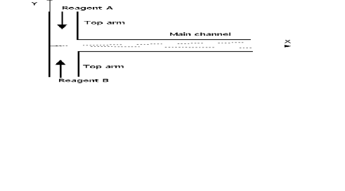
Figure 2: geometry of the microreactor.

The channels were chemically etched in a glass wafer, which was then anodically bonded to a silicon wafer to create a rectangular cross-section. Throughout the experiments discussed here, the channel depth was 10 $\mu$m and the width was 200 $\mu$m. The lengths of the T arms were 1 cm while the main channel was 2 cm long. Two reactant species are introduced through the two top branches of the T and they react as they flow side by side in the main channel. We study the reaction of Calcium ions as reactant A and Calcium Green (CaGreen) from Molecular Probes pro as reactant B (as used, e.g. in Monson and Kopelman (2000)). $\text{Ca}^{2+}$ ions bind with the tracer Calcium Green, significantly increasing its fluorescence rea . Epifluorescence microscopy is used to measure the fluorescence emission, yielding spatial images such as Fig. 3. The flows are driven by syringe pumps which also provide measurements of the flow-rates in each separate branch; those ranged between 30 and 100 nl/mn. Owing to the aspect ratio of the micro-channel, the velocity profile is parabolic across the channel depth and is essentially uniform along $Y$ direction. Furthermore, the low Reynolds number ensures that the fluid flow is invariant in the $x$-direction after some entrance length on the order of the channel thickness.

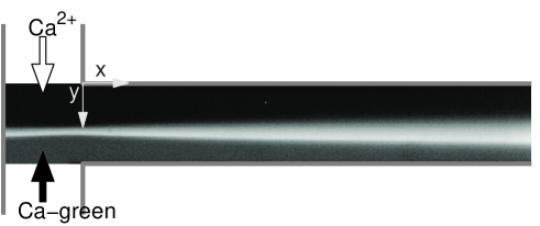
Figure 3: Fluorescent microscopy image of the binding of $\text{Ca}^{2+}$ ions with Calcium-green marker in a T-channel. The channel width is 200 $\mu$m, the depth is 10 $\mu$m. Here, the velocity in the main channel is $U=0.083$ cm/s.

In the conditions in which we operated (i.e. low flow-rates and thin channels) the tracer concentration can be considered as uniform across the channel depth. As a consequence, the concentration fields can be treated as two-dimensional and Eqs. 4 and 6 can be used to describe the system. We tested the two-dimensionality property by performing a series of diffusion experiments (with no reaction) of fluorescein in water. A fluorescein solution and pure water are driven from the two top arms respectively. In the main channel, they form a diffusing interface which progressively broadens downstream. In thick channels, the broadening was found to display the three-dimensional effects discussed in Refs. Kamholz et al. (1999) and Ismagilov et al. (2000), where the diffusion region scales as $x^{1/3}$. In the 10 $\mu$m channels, 2D diffusion theory to agrees well with experiment, with a scaling of the diffusion width as $x^{1/2}$.

The comparison between the 2D theoretical model and the experiment is further justified by the following reasoning: one may consider that the reacting zone is homogeneous across the channel depth in the major part of the region we analyze, for sufficiently thin channels. This argument relies on estimations of the diffusive time across the channel thickness and on the measurements with fluorescein discussed above. We are thus working mostly in the so-called Taylor-Aris regime where the parabolic velocity profile enhances the apparent diffusion coefficient in the flow direction Pagitsas et al. (1986). One may show however that the streamwise diffusion term is still negligible compared to the transverse term, since the streamwise gradients are very weak. These two features justify the use of the model of Eqs. 4 to compare with our experiment.

The diffusion coefficient of Calcium ions is equal to $D_{\text{Ca}^{2+}}=7.9\times 10^{-6}~{}$cm²/s Cussler (1997). The diffusion coefficient of the CaGreen was unknown so we measured it using the method described above, replacing the fluorescein solution with a Calcium Green solution: We checked that the width of the diffused zone increases as the downstream distance raised to the power 1/2, as expected from two-dimensional theory. By fitting the measurements of the width, we obtained an estimate for the Calcium Green diffusion coefficient equal to $3.2\pm 0.3\times 10^{-6}$ cm²/s.

Throughout the experiments, we kept the concentration of $\text{Ca}^{2+}$ constant at [$\text{Ca}^{2+}$]=1 mM, while the concentration of CaGreen was varied in the range $0.1<\text{[CaGreen]}<0.5$ mM. Therefore, the value of $\beta$ varied between $1.4$ and $3.2$, while $\chi$ was fixed at $\chi=1.57$.

Comparison between theory and experiment: A typical concentration field is shown in Fig 3. The black region corresponds to the Calcium solution, the grey one to the CaGreen solution, and the brighter region in the center to the bound Ca-CaGreen complex. The background fluorescence, visible in the lower part of the channel, is due to the fluorescence of unbound CaGreen. The asymmetry in the reaction zone is due to a different rate of diffusion of the reagents, because of their different initial concentrations and different diffusion coefficients. This can be physically explained by noting that the species with the higher diffusion coefficient will diffuse further; furthermore the species with the larger initial concentration will diffuse faster due to the large gradient it experiences. In other words, $\beta$ and $\chi$ both determine the shape of the reaction zone.

We were not able to obtain reliable information on the kinetic coefficient $k$ of the $\text{Ca}^{2+}$-Calcium Green reaction. We thus took $k$ as a free fitting parameter, and adjusted it so as to optimize the agreement between theory and experiment. The best fits were obtained for $k=1.0\pm 0.47\times 10^{6}$ dm³/(mol s), or a length scale $\ell=0.84$ $\mu$m for $\beta=\sqrt{2}$ and $\ell=1.0$ $\mu$m for $\beta=2$. These values of $k$ and $\ell$ are used throughout this letter in comparing the experiments and numerics.

Figure 4 represents the concentration profiles of the Ca-CaGreen complex (dots) measured at various locations downstream, for $\beta=\sqrt{2}$ and 2. The two locations we consider here are $X=278$ and 1128 $\mu$m (for $\beta=\sqrt{2}$ these correspond to $x=32$ and $216$; for $\beta=2$, $x=23$ and $153$). The plots we show are representative of the evolution of the concentration profiles along the downstream axis. The profiles are asymmetric with respect to $Y=0$; in particular the maximum of the concentration is not located at the channel center but is displaced towards the side of the CaGreen solution. For increasing $X$, the reaction zone broadens. The solid lines on Fig. 4 represent the value of $c$ obtained by numerical solutions of Eqs. 4 and 6, by a standard one dimensional finite-difference scheme with time stepping on a personal computer, using the values of the parameters previously established. The offset on the right hand side of the experimental curves is due to the background fluorescence of the unbound CaGreen (reactant $a$). We match this offset in the numerical curves by plotting $ha+c$ rather than just $c$, where $h$ a normalization constant that gives the correct offset. This does not affect the fitting parameters but matches the experimentally measured quantity, i.e. the total fluorescence. We observe good agreement between theory and experiment.

Figure 4: Experimental measurements of the fluorescent intensity (dots) compared with numerical solutions of $c$ (solid lines) at different downstream locations for $\beta=\sqrt{2}$ and $2$. $U=0.334$ cm/s for both cases.

A quantitative measure of the agreement between the simulations and experiments is obtained by looking at some representative quantities for the profiles. In particular, we compare the downstream evolution of three quantities: The position of the maximum, the width at half-height, and the value of the maximum (Fig. 5). These evolutions do not follow simple power laws in the full range of $x$ we consider. However, for $x\gtrsim 30$ dimensionless units, the power laws are better defined. The useful scaling range in the experiments is further limited (at $X\simeq 1200$$\mu$m) by lateral wall effects, thus limiting the range over which a power law can be observed; although the scaling range is too small to obtain a clear exponent, our measurements are consistent with the long time limit analytical theory of Gálfi and Rácz Gálfi and Rácz (1988). The maximum concentration shows a saturation effect at large distances, i.e above $x\simeq 300$. These measurements can be compared with the numerics, plotted as full lines. Fig 5 shows there is good agreement between the theory and the experiment. A similar agreement is obtained different values of $\beta$ and flowrates $U$ we considered.

Figure 5: Evolution of the position of the maximum concentration, width, and value of the maximum with $X$. The $+$ signs are the experiments, while the solid lines are the numerical simulations. Here, $\beta=\sqrt{2}$, $\ell=0.84$ $\mu$m, $U=0.334$ cm/s.

In conclusion, we demonstrate that two-dimensional reaction-diffusion equations with stepwise initial conditions define not only a theoretical problem, but also a physical situation which can be achieved experimentally. Microfluidic reactors are particularly convenient in order to produce such physical situations. Conversely, 2D reaction diffusion equations can be used to determine, from experimental measurements, the relative concentration of the reactants (micro-titration), the diffusion coefficients or the chemical kinetics. In the present case, we demonstrate a determination of the kinetic coefficient $k$ in order to match measured physical quantities (position, width and concentration of the reactant) with numerical predictions. The value of $k$ thus obtained for our system corresponds to a reaction half-time of 1 ms, which is faster than the time scales that can be resolved in a stopped-flow apparatus. This indicates that the present approach can be used for analyzing fast chemical kinetics.

The authors acknowledge technical help from Bertrand Lambollez, Jean Rossier and Thibault Colin, and useful discussions with Martin Bazant.

References

- (1) Present address: Laboratoire d’Hydrodynamique (LadHyX), Ecole Polytechnique, 91128 Palaiseau Cedex, France. email: baroud@ladhyx.polytechnique.fr.
- Gálfi and Rácz (1988) L. Gálfi and Z. Rácz, Phys. Rev. A 38, 3151 (1988).
- Taitelbaum et al. (1992) H. Taitelbaum, Y. Koo, S. Havlin, R. Kopelman, and G. Weiss, Phys. Rev. A 46, 2151 (1992).
- Koo and Kopelman (1991) Y.-E. L. Koo and R. Kopelman, J. Stat. Phys. 65, 893 (1991).
- Park et al. (2001) S. Park, S. Parus, R. Kopelman, and H. Taitelbaum, Phys. Rev. E 64, 055102 (2001).
- Léger et al. (1999) C. Léger, F. Argoul, and M. Bazant, J. Phys. Chem. 103, 5841 (1999).
- Kamholz et al. (1999) A. Kamholz, B. Weigl, B. Finlayson, and P. Yager, Anal. Chem. 71, 5340 (1999).
- Cussler (1997) E. Cussler, Diffusion, Mass transfer in fluid systems (Cambridge University Press, Cambridge, 1997), 2nd ed.
- (9) See http://www.probes.com/.
- Monson and Kopelman (2000) E. Monson and R. Kopelman, Phys. Rev. Lett. 85, 666 (2000).
- (11) The pH of the solutions is stabilized at 7.5 by using a Tris buffer. Furthermore, traces of Calcium in the Ca-green solution are neutralized by adding excess EDTA.
- Ismagilov et al. (2000) R. Ismagilov, A. Stroock, P. Kenis, G. Whitesides, and H. Stone, Appl. Phys. Lett. 76, 2376 (2000).
- Pagitsas et al. (1986) M. Pagitsas, A. Nadim, and H. Brenner, Physica A 135, 533 (1986).