A computational theory for the classification of natural biosonar targets based on a spike code

Abstract

A computational theory for classification of natural biosonar targets is developed based on the properties of an example stimulus ensemble. An extensive set of echoes ($84\,800$) from four different foliages was transcribed into a spike code using a parsimonious model (linear filtering, half-wave rectification, thresholding). The spike code is assumed to consist of time differences (interspike intervals) between threshold crossings. Among the elementary interspike intervals flanked by exceedances of adjacent thresholds, a few intervals triggered by disjoint half-cycles of the carrier oscillation stand out in terms of resolvability, visibility across resolution scales and a simple stochastic structure (uncorrelatedness). They are therefore argued to be a stochastic analogue to edges in vision. A three-dimensional feature vector representing these interspike intervals sustained a reliable target classification performance (0.06% classification error) in a sequential probability ratio test, which models sequential processing of echo trains by biological sonar systems. The dimensions of the representation are the first moments of duration and amplitude location of these interspike intervals as well as their number. All three quantities are readily reconciled with known principles of neural signal representation, since they correspond to the center of gravity of excitation on a neural map and the total amount of excitation.

1 Problem

This work explores a computational theory for a set of biosonar tasks faced by bats. Based on an extensive set of real world echo data, it develops and explores a parsimonious solution for a well-defined, yet widely useful set of sensing problems posed by extended, multi-faceted sonar targets. In particular, classification of foliages from different species of deciduous trees is performed. Such foliages are examples of ubiquitous, natural sonar targets in the habitats of many bat species. The ability to classify them is immediately relevant to biological tasks like landmark identification or habitat evaluation (e.g., based on a probability estimate for the presence of a certain prey) in general. Furthermore, in any other estimation task where the informative signal properties depend on foliage class, a hypothesis for the latter could be employed to enhance performance. Examples of other related biological tasks likely to be performed to some extent by bats could be related to obtaining information about the convex hull of an extended target or finding passageways (e.g., in collision avoidance, contour following or path planning).

Multi-faceted targets, which place moderate to large numbers of reflectors in the sonar beam, pose a special challenge for sonar systems limited to sparse spatial sampling with only two receivers: Echoes received by each ear are superpositions of contributions from all reflectors within the beam (moderate facet numbers would be on the order of $10$, large numbers on the order of $10^{2}$ to $10^{4}$). Reconstruction of target geometry/reflector location would require both deconvolution (bats use chirping sonar pulses) as well as estimating reflector placement from a collection of integrals over prolate spheroidal surfaces. The second step in particular - besides relying on simplifying assumptions [1] not necessarily met in natural biosonar targets - will remain an ill-posed problem until a sufficiently large number of such integrals has been gathered. The behavioral patterns seen in bats may not leave enough room for this prior to the time when a class estimate is due. Besides the issue of possible intractability under such constraints, a parsimony argument stands against reflection-tomographic solutions as a model for biosonar function in these tasks: Position, orientation and shape of individual reflectors in a foliage are not immediately relevant to the behavioral goals of the animal and therefore reconstruction of these target features would be a detour into yet another representation from which the relevant variables (identity of a landmark, collision risk, presence and location of a passageway, etc.) would still have to be estimated. Parsimonious models for biosonar sensing should neither recover irrelevant detail about a target explicitly nor should they rely on intermediate representations which contain an excessive amount of such detail.

If the geometry of a target is not known, it is impossible to predict the waveform or other individual properties of subsequent echoes received from it at different viewing positions. In this sense, the echoes from foliages have to be viewed as realizations of random processes, despite their origin in a deterministic reflection process. Consequently, the particular problem at hand here is to classify natural targets (foliages) based on random input signals, where the individual waveforms will in general not contain any deterministic patterns beyond the sonar pulse used to generate them [2]. The computational theory presented here deals with performing this task based on a simple spike code. In contrast to a previous attempt at solving this problem [3], the present work is based on a thorough characterization of the stimulus ensemble, explores the fundamental nature of the employed coding scheme and evaluates the performance of the proposed estimator quantitatively.

Since bats emit trains of pulses, this evaluation of the proposed estimator will take the form of an m-ary sequential probability ratio test. In this way, it will be explored to what extent bats could make use of the sequential information that they receive in their pulse trains.

2 Aim of the paper

The work presented here solves the problem outlined above based on features derived from a parsimonious model of the signal representation formed in the auditory system. This serves a dual purpose: First, it helps to outline a solution space for classification of natural targets into which the specific solutions adopted by bats must fall. Second, it employs known functional principles from biology as a means to discover good solutions to fundamental problems with wider relevance to technical applications.

Like most mobile animals, bats possess navigation skills and the ability to make habitat choices. This work demonstrates echo features which have the necessary explanatory power to qualify as a tangible hypothesis for the basis of these skills. The fact that these features have been proven effective with realistic, physical data, makes them excellent candidates for testing their actual use by bats in behavioral and neurophysiological experiments. Since the work presented here is a computational theory, it is concerned with principle feasibility only and does not consider functional properties of the auditory system with no specific relevance to the particular problem at hand.

The specific biosonar sensing problem under consideration can be taken as an example of a wider class of random signal classification problems. Related problems arise in technical applications, e.g., biomedical ultrasound diagnosis or channel estimation for wireless communication links. Bats provide an existence proof for the solutions to problems associated with the tasks the animals face and hence offer a convenient access route to more general solutions of possible technological relevance.

3 Approach

The approach taken here is to employ a biomimetic sonar observer which selectively replicates those fundamental functional properties of its biological paragon that are relevant to the particular problem at hand. The biomimetic observer is used to collect large echo data sets from extended, natural targets over a realistic range of viewing positions. In this way, the natural variability can be exhausted for these particular examples and statistical characterizations of the stimulus ensemble can be obtained with sufficient confidence even if they require a large number of data points (e.g., non-parametric estimates of multivariate probability density functions). In the present work, the stimulus ensemble is characterized at the level of spike code features. The spike code features are the result of processing the experimental stimulus ensemble with a parsimonious spike generation model. Consequently, the identified features are salient under a minimum number of assumptions as well.

3.1 Biomimetic sonar system and data

Hedges of four deciduous tree species, sycamore (Platanus hybrida), linden (Tilia cordata), field maple (Acer campestre), and hornbeam (Carpinus betulus), were constructed from large individual branches. These targets extended between 2 and 3 m in width, $\sim 2\,\mathrm{m}$ in height and between 1.6 and 2 m in depth. Each hedge was composed of 3 to 8 individual branches, which were arranged to fill the given volume in a semi-natural fashion. The targets were considerably larger along every dimension than those employed by [4] in a study on foliage classification with CWFM sonar, where target depth appeared to be less than 45 cm, making individual plant shape a likely determinant of the observed features. Just like in a natural forest, where individual trees are almost certain to extend beyond the volume which can be illuminated by an individual sonar pulse, this was not the case here.

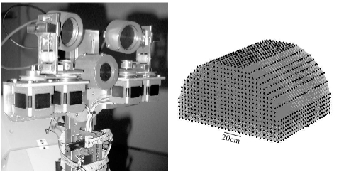
Figure 1: Experimental setup and spatial sampling paradigm. Left: biomimetic sonar head; right: spatial arrangement of points (black dots) at which echoes were sampled. The gray surfaces represent the convex hull of all sampling positions. The target hedge was positioned opposite to the frontal face of the sampled volume.

The targets were scanned in three dimensions with a biomimetic sonar head (see figure 1 left) mounted on a humanoid robot arm. The sonar head consisted of three electrostatic transducers, one for emission (Polaroid 7000) and two for reception (Polaroid 600). The receivers were positioned 12.5 cm apart (measured between aperture centers); the emitter was placed halfway between and 4.5 cm below the two receivers. The head was moved within a work envelope of 116 cm width, 64 cm height and 96 cm depth (perpendicular to the hedge). Since the two upper edges of the work envelope perpendicular to the target were rounded due to lack of reachability, the entire scanned volume was $\sim 0.6\,\mathrm{m^{3}}$ (as opposed to $\sim 0.71\,\mathrm{m^{3}}$ for a cuboid of the given edge lengths). The minimum target range within this work envelope was $\sim 1\,\textrm{to}\,1.3\,\mathrm{m}$.

The directivity of the employed electrostatic transducers is modeled well by an (unbaffled) piston [5, 6], which is also in fairly good agreement with data from at least two bat species [7, 8]. The first-null beamwidth is 40 ° for the emitter and 30 ° for the receivers. These beams correspond to sonar footprint diameters of $\sim 73\,\mathrm{cm}$ and $\sim 54\,\mathrm{cm}$ in 1 m distance, respectively (assuming normal incidence). While both emitter and receivers were always oriented towards the hedge, this did not guarantee normal incidence since the local orientation of the hedge surface varied and the data can be expected to represent a wider range of grazing angles.

The volume enclosed by the work envelope was sampled every 4 cm along the width, height and depths dimensions (see figure 1 right), resulting in $10\,600$ positions and a total of $21\,200$ echoes received at the two “ears” for each target. The total data set size for all four targets is therefore $84\,800$. Echo waveforms were digitized with 1 MHz sampling rate and 12 Bit resolution. Spectrograms of example echoes are shown in figure 2.

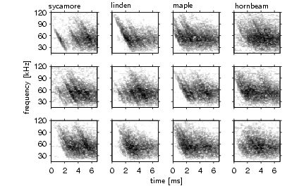
Figure 2: Spectrograms of example echoes. For each of the four target classes (columns), three examples (rows) are shown. The spectrograms were computed using a Hamming window spanning 512 samples, windows were spaced for an overlap of $3/4$ of their width. All spectrograms were normalized for equal maximum power and the dynamic range was restricted to 50 dB.

Regardless of distance between recording positions, all echoes in the data set showed very low correlations determined over all possible lags ($\tau$) as

$$\hat{\rho}=\frac{\max\{|\hat{C}_{xy}(\tau)|\}}{\sqrt{\hat{E}_{x}\hat{E}_{y}}},$$ (1)

where $C_{xy}$ is the biased estimate of the cross-covariance between the two echoes [9] and $\hat{E}_{x},\hat{E}_{y}$ are estimates of their respective energies (Figure 3).

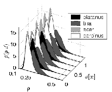
Figure 3: Conditional probability density function estimates $\hat{p}(\rho|d)$ of the maximum correlation coefficient $\rho$ (over all lags, see (1)) between echoes conditioned upon the distance $d$ between the recording positions. Density estimates were based on a random sample of $1\,000$ echo pairs per distance bin and foliage class and were obtained with normal kernels (smoothing bandwidths between $0.004$ and $0.012$), the asymptotic mean integrated squared error (AMISE, the first order term in a series expansion of the mean integrated square error, [10]) ranges between $0.018$ and $0.067$.

A thorough reshuffling of weights for each reflector due to the directivities of reflectors and transducers is the likely cause for these small correlation distances, which do not exceed the sampling distance chosen here for any correlation value of practical relevance.

3.2 Biological signal processing model

The signal processing model used for characterizing the stimulus ensemble at a spike code level consists of two stages: preprocessing and spike generation. Both stages were simplified to reflect only essential signal processing steps.

In the preprocessing stage, the reflector sequence (impulse response) of the target was filtered by four bandpass filters in series: the emitted pulse, the transfer functions of emitter and receiver, as well as an auditory bandpass filter model. The emitted pulse was a linearly frequency modulated chirp sweeping across almost the entire passband of the transducers (from 120 kHz to 20 kHz) in 3 ms. As the first major simplification introduced here, only a single bandpass channel in the auditory representation of this wideband signal is considered. A 4-th order gammatone filter with center frequency $f_{c}$ and -3 dB quality $Q$ (ratio of $f_{c}$ and the filter bandwidth at -3 dB) was used as an accepted standard [11] for modeling auditory filters, although the specific shape of the transfer function is of little relevance to the features that this work focuses on. The combined effect of all linear signal processing stages can be described as filtering the reflector sequence with a chirplet, which is the result of convolving all four impulse responses (Figure 4). Since the passbands of the transducer transfer functions are broad compared to that of the auditory filter model, their effect on the combined impulse response is negligible for any particular auditory bandpass channel observed in isolation. Depending on the width of the channel’s passband, the frequency sweep of the pulse will also be negligible, resulting in the combined impulse response being approximately a wavelet of constant carrier frequency.

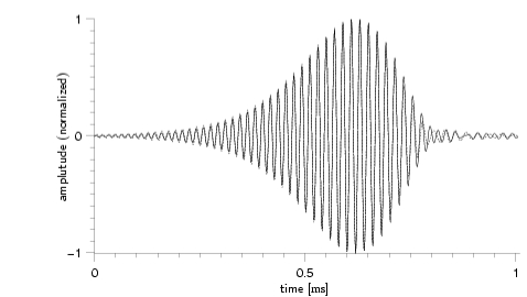
Figure 4: Measured combined impulse response (chirplet) for sonar pulse, emitter, receiver, and auditory bandpass filter model (——). The auditory bandpass model parameters $f_{c}=50\,\mathrm{kHz}$ and $Q_{-3\,\mathrm{dB}}=10$ are used throughout the reported work and result in a -3 dB impulse response duration of $\sim 260\,\mathrm{\textrm{\textmu}s}$. The actual data of the combined impulse response was collected by directing the sonar head at a plane in $\sim 1.8\,\mathrm{m}$ distance; in the graph, it is compared to a simplified model which omits the transducer transfer functions (-  -  -  -).

Preprocessing was completed by an approximate envelope extraction performed as half-wave rectification and subsequent lowpass filtering [12]. To the extent to which this procedure provides for an undistorted demodulation of the signal [13], the effect of the lowpass filter is equivalent to a further increase in the quality of the original bandpass filter. The employed lowpass filter was a 1st order recursive lowpass filter (“leaky integrator”) with time constant $\tau$. Altogether, the simplified preprocessing model is described by a parameter triplet of $f_{c},Q$ and $\tau$. Throughout this work, the center frequency of the auditory model filter was set to 50 kHz, close to the maximum of the transducer transfer function. The chosen filter quality of 10 at -3 dB is approximately commensurate with findings from some nuclei in the lower auditory brainstem [14]. Although integration times in bats have been probed with both psychoacoustic and physiological methods [15], it is difficult to obtain an estimate for the parameter $\tau$ of the present model from these experimental results. Therefore, the entire range of plausible values was explored here (from $\tau=0$ to 10 ms, s. below) and the cases $\tau=0$ (no integration) and $\tau=3\,\mathrm{ms}$ (significant smoothing, yet far from perfect integration) are shown throughout as examples to assess the influence of further integration/narrowing of the passband on all reported results. In evaluating model performance for target classification (see section 5), a broader sample of model parameter combinations ($f_{c},Q,\tau$) was used ($f_{c}=\left\{40\,\mathrm{kHz};45\,\mathrm{kHz};50\,\mathrm{kHz};55\,\mathrm{kHz};60\,\mathrm{kHz};65\,\mathrm{kHz}\right\},Q=\left\{10;15;20;25;30;35\right\},\tau=\left\{0;1\,\mathrm{ms};3\,\mathrm{ms};5\,\mathrm{ms};7\,\mathrm{ms};10\,\mathrm{ms}\right\}$) to investigate how sensitive performance is to changes in model parameters.

Spike encoding of the preprocessed signal was modeled as parsimoniously as preprocessing: The input signal was normalized so that only waveform shape and not energy was considered. Therefore, no compensation for initial target range and associated spreading losses was required. Spike times were determined by thresholding the signal. Together with the specific lowpass filter chosen for the envelope extraction step, this amounts to an “integrate and fire” model, which is a simplification of the Hodgkin-Huxley equations [16]. The sufficiency of this model for the problem at hand will be justified below from the nature of the features (Section 4). As a second major simplification, only spikes triggered by the initial transient, i.e., the “onset response” of a neuron will be considered. This simplification is necessitated by the lack of relevant data on neural refractoriness in bats.

A single spike time is obviously not sufficient for target classification, since it would inevitably confound target range and class. To retain the simplifications made already (only one bandpass channel, only one spike triggered by the initial transient in each neuron), a population of neurons with different thresholds was chosen as a way to diversify the code according to the needs of target classification. The adopted model is therefore an amplitude-discrete sampling of the “inverse function” (considering the lowest/earliest branches only) of the preprocessed signal up to its maximum; the signal beyond the maximum is ignored.

Feature extraction from spike times uses only time differences within the neural response to an echo; using an external reference can provide a range estimate, but has no immediate relevance for target classification (An indirect influence is possible, should classification features be range-dependent - this remains to be explored). Neural circuitry for estimation of monaural time differences is well established in bats, e.g., in the context of ranging, where comparatively long time-of-flight values have been found represented (few milliseconds to more than 10 ms [17, 18]). Mammals with sufficient ear distances can determine direction-of-arrival by binaural time differences, typically in the sub-millisecond range ($1\,\mathrm{ms}$ corresponds to $\sim 34\,\mathrm{cm}$ distance already). In bats, indications have been found that the respective neural structures (MSO) can deal with time differences both in the sub-millisecond range and beyond [19]. However, this was established only for sinusoidal amplitude modulation. In contrast to this, the computational work presented here emphasizes the importance of aperiodic, random time differences within echoes, which can take values comparable to what is typically considered in binaural difference evaluation as well as in ranging.

Specifically, the model consists of $M$ thresholds $a_{m}$, where $a_{n}>a_{m}$ for $n>m$. These thresholds give rise to $M(M-1)$ possible non-zero interspike intervals $\Delta\left(\alpha_{m},\alpha_{n}\right)$ between the times of crossing the $m$-th and the $n$-th threshold. For specification of the model, two functions must be chosen; one for threshold placement on the amplitude axis and one for selecting the threshold pairs for which the $\Delta\left(\alpha_{m},\alpha_{n}\right)$ are computed (i.e., the wiring of the neural delay-lines/coincidence detectors). Unfortunately, no biological data is available on either of these two functions. As a remedy, thresholds were placed equidistantly at least one standard deviation of the noise amplitude apart. Since the signal-to-noise ratio of the experimental setup, which was limited by the sound channel and not the electronics, was better than $60\,\mathrm{dB}$ for the larger echo amplitudes encountered, $M=1,024$ (chosen as an integer power of 2) thresholds were employed altogether. Bats were found to have between $700$ and $2\,160$ inner hair cells and between $13\,400$ and $55\,300$ spiral ganglion cells for covering the entire hearing range of the respective species; divergence ratios from inner hair cells to spiral ganglion cells range from 11 to 79 [20]. Since it is not known how many neighboring channels could be pooled based on the similarity of their transfer functions, it is likewise hard to estimate how many neurons would be available for thresholding the output of one bandpass channel. From the numbers given and the similar constraints on the signal to noise ratio in the sound channel, it is unlikely though, that this model sacrifices any amplitude resolution that bats may have.

Once thresholds have been placed (a vector of threshold values has been chosen), the matrix of all possible $\Delta\left(\alpha_{m},\alpha_{n}\right)$ for any echo is completely determined as well. Since this matrix has odd symmetry, i.e., $\Delta\left(\alpha_{m},\alpha_{n}\right)=-\Delta\left(\alpha_{n},\alpha_{m}\right)$, considering e.g., the upper triangular part suffices. Further more, the entire matrix can be reconstructed exactly from the elements on the first diagonal as

$$\Delta\left(\alpha_{m},\alpha_{n}\right)=\sum_{k=m}^{n-1}\Delta\left(\alpha_{k},\alpha_{k+1}\right).$$ (2)

In this sense interspike intervals $\Delta\left(\alpha_{m},\alpha_{m+1}\right)$ generated by subsequent exceedance of neighboring thresholds $a_{m},a_{m+1}$ may be regarded as elementary intervals. All other intervals which may be generated in a bat’s brain are just sums of these variables. Equation (2) describes a resolution pyramid, in which detail is lost as the diagonal under consideration is moved away from the main diagonal. While the matrix of all possible $\Delta\left(\alpha_{m},\alpha_{n}\right)$-values is completely determined by its first diagonal and hence highly redundant, it may be perceptually relevant, if small $\Delta\left(\alpha_{m},\alpha_{m+1}\right)$ fall below the resolution limit, but not their sums.

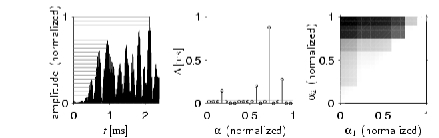
Figure 5: Example for the application of the employed spike generation model. Left: the normalized waveform is thresholded up the its maximum; center: duration of interspike intervals $\Delta\left(\alpha_{m},\alpha_{m+1}\right)$ for neighboring thresholds; right: matrix of all possible interspike intervals for the given set of thresholds.

4 Code properties

4.1 Elementary interspike intervals

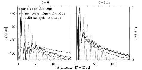
Figure 6: Probability density function estimates for the elementary interspike intervals $\Delta\left(\alpha_{m},\alpha_{m+1}\right)$ for the four foliage types sycamore (○), linden (□), maple (▽), hornbeam ($\ast$). Shown are kernel density estimates using a normal kernel with $1\,\mathrm{\textrm{\textmu}s}$ smoothing bandwidth. Dashed line: normalized autocorrelation function $R_{xx}(\tau)/\sigma^{2}$ of the chirplet shown in figure 4.

Filtering the reflector sequence with the chirplet representing all linear channel effects (Figure 4) introduces a prominent periodicity corresponding to the carrier period of the auditory bandpass model (here $T=20\,\mathrm{\textrm{\textmu}s}$). This periodicity is clearly visible in the probability density function of the elementary interspike intervals $\Delta\left(\alpha_{m},\alpha_{m+1}\right)$ (Figure 6). Since the probability density function has two nulls at $\leavevmode\nobreak\ \sim 10\,\mathrm{\textrm{\textmu}s}$ and $\leavevmode\nobreak\ \sim 30\,\mathrm{\textrm{\textmu}s}$ for $\tau=0$ and its most pronounced notches are in the same places for $\tau=3\,\mathrm{ms}$, a clear distinction can be made between three different types of interspike intervals depending on how the two delimiting spike times are arranged with respect to the carrier period (Figure 6):

• For same slope intervals flanking spikes are triggered by the same rising flank of a positive half-wave; for the particular channel center frequency chosen here, $\Delta\left(\alpha_{m},\alpha_{m+1}\right)\leq 10\,\mathrm{\textrm{\textmu}s}$ in this interval category.

• For next cycle intervals flanking spikes are triggered by subsequent positive half-waves. For the particular channel center frequency chosen here, next cycle intervals must have values such that $10\,\mathrm{\textrm{\textmu}s}\leq\Delta\left(\alpha_{m},\alpha_{m+1}\right)\leq 30\,\mathrm{\textrm{\textmu}s}$.

• For distant ($>1$) cycle intervals flanking spikes are triggered more than one carrier cycle apart, hence $\Delta\left(\alpha_{m},\alpha_{n}\right)\geq 30\,\mathrm{\textrm{\textmu}s}$ for distant cycle intervals.

For next and distant cycle $\Delta\left(\alpha_{m},\alpha_{m+1}\right)$, the inverse function of the waveform (counting only lower branches, see section 3.2 and figure 5) has discontinuities, i.e.,

$$\lim_{|\alpha_{n}-\alpha_{m}|\rightarrow 0}{\Delta\left(\alpha_{m},\alpha_{n}\right)}=C$$ (3)

as long as the discontinuity of the inverse function remains bracketed by $\left[\alpha_{m},\alpha_{n}\right]$. This implies that such discontinuities remain visible in any $\Delta\left(\alpha_{m},\alpha_{n}\right)$ where the corresponding thresholds $\alpha_{m},\alpha_{n}$ bracket them. Because they are discontinuity-based, next and distant cycle $\Delta\left(\alpha_{m},\alpha_{m+1}\right)$ are invariant under any monotonic non-linear transform of the signal amplitude, an important property as the auditory system is known to perform non-linear compression [12]. Unlike same slope and next cycle $\Delta\left(\alpha_{m},\alpha_{m+1}\right)$, the durations of distant cycle $\Delta\left(\alpha_{m},\alpha_{m+1}\right)$ are not strictly tied to the carrier cycle, because the autocorrelation of the chirplet ($R_{xx}(\tau)$, superposed in figure 6) decays and the echo waveform decorrelates.

Despite the comparative rarity of distant cycle $\Delta\left(\alpha_{m},\alpha_{m+1}\right)$ evident from figure 6, it is almost certain that at least one distant cycle $\Delta\left(\alpha_{m},\alpha_{m+1}\right)$ is present in the response to any given echo (Figure 7).

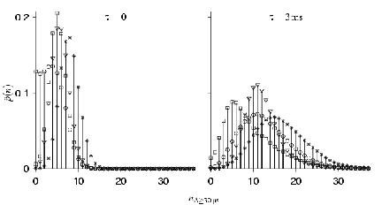
Figure 7: Probability density function estimates for the number of distant cycle $\Delta\left(\alpha_{m},\alpha_{m+1}\right)\geq 30\,\mathrm{\textrm{\textmu}s}$ per echo. The probabilities for at least one distant cycle interspike interval $P\left\{n_{\Delta\geq 30\,\mathrm{\textrm{\textmu}s}}\geq 1\right\}$ is $\sim 0.94$ for sycamore and $\tau=0$, for all others $P\left\{n_{\Delta\geq 30\,\mathrm{\textrm{\textmu}s}}\geq 1\right\}\geq 0.99$. Estimates used a normal kernel with smoothing bandwidth $0.82-0.99$, AMISE $<0.0015$. See figure 6 for symbols denoting target class.

For the chosen threshold spacing, this is true for any smoothing constant and the expected number of distant cycle thresholds shows a saturating increase with increasing time constant $\tau$ (Figure 8).

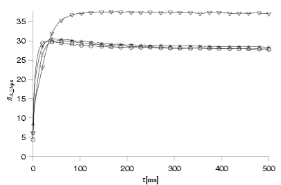
Figure 8: Effect of lowpass filtering time constant ($\tau$) on the expected number $\bar{n}_{\Delta\geq 3\,\mathrm{\textrm{\textmu}s}}$ of distant cycle $\Delta\left(\alpha_{m},\alpha_{m+1}\right)$. The estimates are based on $N=500$ randomly chosen echoes for each value of $\tau$ and each foliage class. See figure 6 for symbols denoting target class.

If instead the limit of $\tau\rightarrow\infty$ and $|\alpha_{n}-\alpha_{m}|\rightarrow 0$, i.e., perfect, “non-leaky” integration and infinitely narrow spacing of thresholds, was to be considered, only next cycle elementary $\Delta\left(\alpha_{m},\alpha_{m+1}\right)$ would be retained, because they correspond to the negative half-cycles of the waveform which were set to zero by the half-wave rectification. For finite threshold spacing, the situation is quite different and distant cycle $\Delta\left(\alpha_{m},\alpha_{m+1}\right)$ do not disappear as a consequence of smoothing. Both robustness and relative rarity of distant cycle $\Delta\left(\alpha_{m},\alpha_{m+1}\right)$ are due to the fact that these $\Delta\left(\alpha_{m},\alpha_{m+1}\right)$ are indicative of an extended trough in the echo waveform. For any given echo, there will be but a few of such troughs (hence the rarity), but since they are low-frequency phenomena, they are robust against lowpass smoothing.

4.2 Compound interspike intervals

Usage of distant cycle $\Delta\left(\alpha_{m},\alpha_{m+1}\right)$ does not place demanding constraints on spike time resolution, whereas access to the shorter individual next cycle intervals and in particular same slope intervals does. Neurophysiological data on spike timing accuracy in the auditory nerve of bats appears to be lacking, however. In cats, minimum standard deviations of onset spike responses were found to be not much lower than $\sim 100\,\mathrm{\textrm{\textmu}s}$ [21], making individual $\Delta\left(\alpha_{m},\alpha_{n}\right)$ from the same slope and next cycle class appear an unlikely substrate for target class estimation. Such small, elementary $\Delta\left(\alpha_{m},\alpha_{m+1}\right)$ could achieve guaranteed perceptual saliency, however, if the amplitude range spanned by a threshold pair was widened. In this case, longer, resolvable compound intervals (see (2)) could emerge as a sum of elementary $\Delta\left(\alpha_{m},\alpha_{m+1}\right)$ with the value of the sum being dominated by contributions from same slope and next cycle $\Delta\left(\alpha_{m},\alpha_{m+1}\right)$. To explore this possibility, compound $\Delta\left(\alpha_{m},\alpha_{n}\right)$ which exceeded some minimum length $\eta$

$$\Delta\left(\alpha_{m},\alpha_{n}\right)=\sum_{k=m}^{n-1}\Delta\left(\alpha_{k},\alpha_{k+1}\right)\geq\eta$$ (4)

were selected and a ratio $r$ which describes the contribution of elementary $\Delta\left(\alpha_{m},\alpha_{m+1}\right)\leq\nu$ (i.e., same slope or same slope or next cycle intervals) was computed as

$$r=\frac{\sum_{k=m}^{n-1}\Delta\left(\alpha_{k},\alpha_{k+1}\right)I_{\Delta\left(\alpha_{k},\alpha_{k+1}\right)\leq\nu}}{\sum_{k=m}^{n-1}\Delta\left(\alpha_{k},\alpha_{k+1}\right)},$$ (5)

where $I$ is the indicator function. The expected value of this ratio was found to depend on the choice of $m$ and $n>m$ (see examples in the left subgraphs in figure 9) and therefore the expected overall impact of same slope and next cycle interspike intervals on the interspike intervals actually read out cannot be estimated without knowing the distribution of readout connections over all possible pairs of incoming neurons. The maximum ratio is a distribution-free measure, however, and it indicated that same slope $\Delta\left(\alpha_{m},\alpha_{m+1}\right)$ have little impact on long compound $\Delta\left(\alpha_{m},\alpha_{n}\right)$ regardless of the smoothing time constants (Figure 9).

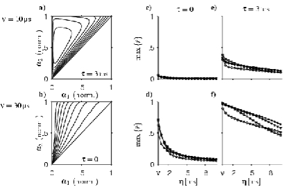
Figure 9: Ratio $r$ of durations of elementary $\Delta\left(\alpha_{m},\alpha_{m+1}\right)\leq\nu$ in compound $\Delta\left(\alpha_{m},\alpha_{n}\right)$ to the total duration of the compound $\Delta\left(\alpha_{m},\alpha_{n}\right)\geq\eta$ (see (5)). Left graphs: examples of expected values of $r$ as a function of threshold locations $\alpha_{1},\alpha_{2}$, a) $\nu=10\,\mathrm{\textrm{\textmu}s}$ (same slope intervals) and $\tau=3\,\mathrm{ms}$, b) $\nu=30\,\mathrm{\textrm{\textmu}s}$ (same slope and next cycle intervals) and $\tau=3\,\mathrm{ms}$. Center and right graphs: maximum of $r$ over all threshold pairs: c) $\nu=10\,\mathrm{\textrm{\textmu}s},\tau=0$, d) $\nu=30\,\mathrm{\textrm{\textmu}s},\tau=0$, e) $\nu=10\,\mathrm{\textrm{\textmu}s},\tau=3\,\mathrm{ms}$, f) $\nu=30\,\mathrm{\textrm{\textmu}s},\tau=3\,\mathrm{ms}$. See figure 6 for symbols denoting target class.

Next cycle elementary $\Delta\left(\alpha_{m},\alpha_{m+1}\right)$ could be the dominating component of long compound $\Delta\left(\alpha_{m},\alpha_{n}\right)$, if a long smoothing time constant was chosen. On the basis of these results, same slope elementary $\Delta\left(\alpha_{m},\alpha_{m+1}\right)$ are of doubtful perceptual salience, both in isolation and in compound intervals. Next cycle elementary $\Delta\left(\alpha_{m},\alpha_{m+1}\right)$ are of doubtful perceptual salience in isolation, but may be a dominating component in longer compound $\Delta\left(\alpha_{m},\alpha_{n}\right)$, if long integration times are chosen. Therefore, in the next section (Section 4.3), only next and distant cycle $\Delta\left(\alpha_{m},\alpha_{m+1}\right)$ are retained for further consideration.

4.3 Interspike interval random process

Retaining only next and distant cycle $\Delta\left(\alpha_{m},\alpha_{m+1}\right)$, each echo is represented by a random sequence of variable length, since for each $\Delta\left(\alpha_{m},\alpha_{m+1}\right)$-class more than one $\Delta\left(\alpha_{m},\alpha_{m+1}\right)$ per echo is likely (see Figures 7,8 for distant cycle $\Delta\left(\alpha_{m},\alpha_{m+1}\right)$; next cycle $\Delta\left(\alpha_{m},\alpha_{m+1}\right)$ are more common than distant cycle $\Delta\left(\alpha_{m},\alpha_{m+1}\right)$, see figure 6). Associated with each $\Delta\left(\alpha_{m},\alpha_{m+1}\right)$ is a position along the amplitude axis marking the location of the two neighboring thresholds the flanking spikes were triggered at.

The random sequences formed by next and distant cycle $\Delta\left(\alpha_{m},\alpha_{m+1}\right)$ differ in their statistical properties: Next cycle $\Delta\left(\alpha_{m},\alpha_{m+1}\right)$ show a strong pairwise dependence between neighboring values as well as correlations of varying strength over the entire sequence, whereas distant cycle $\Delta\left(\alpha_{m},\alpha_{m+1}\right)$ random sequences are uncorrelated and at least pairwise independent (Figures 10,11).

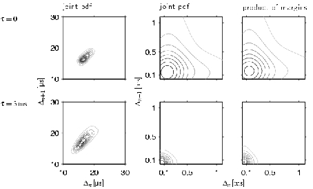
Figure 10: Estimates of the joint probability density function for neighboring $\Delta\left(\alpha_{m},\alpha_{m+1}\right)$ in the response to echoes from sycamore foliage. The contour levels are spaced linearly between 10% and 90% of the density functions’ maxima. Estimates are based on $N=21\,200$ echoes.

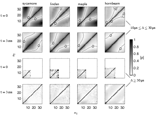
Figure 11: Correlation matrix estimates for the vectors of next cycle and distant cycle $\Delta\left(\alpha_{m},\alpha_{m+1}\right)$. The matrices show estimates of the correlation coefficient magnitude $|\rho|$ for interval duration as a function of positions $n_{1},n_{2}$ in the interval sequence. The top two rows show correlation matrix estimates for next cycle $\Delta\left(\alpha_{m},\alpha_{m+1}\right)$ generated with smoothing time constants $\tau=0$ (first row) and $\tau=3\,\mathrm{ms}$ (second row). The bottom two rows show the same estimates for distant cycle $\Delta\left(\alpha_{m},\alpha_{m+1}\right)$. Estimates are based on $N=21\,200$ echoes for each foliage class; the number of realizations for sequences of a particular minimum-length varies, however, and leads to a higher estimator variance on the edges of the covariance matrices for $\Delta\geq 30\,\mathrm{\textrm{\textmu}s}$ and $\tau=0$.

Therefore, the distant cycle $\Delta\left(\alpha_{m},\alpha_{m+1}\right)$ random sequences have a much simpler statistical structure than next cycle $\Delta\left(\alpha_{m},\alpha_{m+1}\right)$, which facilitates the design of a classifier. For this reason, as well as because of their low resolution requirements, they will be used in the next section to attempt target classification based on output of the spike generation model (see section 5).

5 Classification based on distant-cycle interspike intervals

The results outlined in the previous sections demonstrate that distant-cycle $\Delta\left(\alpha_{m},\alpha_{m+1}\right)$ offer advantages both for actual use by biological systems (low resolution requirements, high visibility in compound $\Delta\left(\alpha_{m},\alpha_{n}\right)$) as well as for further studies (uncorrelated random sequences). The decisive question is whether the distant-cycle $\Delta\left(\alpha_{m},\alpha_{m+1}\right)$ also contain sufficient information on target class. To answer this question, target classification was attempted using an ad-hoc feature selection approach, which is unlikely to make optimum use of the random sequences, but serves its purpose of demonstrating feasibility in case of success.

Each spike response to an echo was represented by three features: first moment estimates for distant cycle $\Delta\left(\alpha_{m},\alpha_{m+1}\right)$ interval length ($\bar{\Delta}$) and amplitude location ($\bar{\alpha}$) as well as the number ($n_{\Delta\geq 30\,\mathrm{\textrm{\textmu}s}}$) of distant cycle $\Delta\left(\alpha_{m},\alpha_{m+1}\right)$ in the spike response to an echo:

$$\eqalign{n_{\Delta\geq 30\,\mathrm{\textrm{\textmu}s}}&=\sum_{m}I_{\Delta\left(\alpha_{m},\alpha_{m+1}\right)\geq 30\,\mathrm{\textrm{\textmu}s}}\\ \bar{\alpha}&=\frac{1}{2N}\sum_{m}\left(\alpha_{m+1}-\alpha_{m}\right)I_{\Delta\left(\alpha_{m},\alpha_{m+1}\right)\geq 30\,\mathrm{\textrm{\textmu}s}}\\ \bar{\Delta}&=\frac{1}{N}\sum_{m}\Delta\left(\alpha_{m},\alpha_{m+1}\right)I_{\Delta\left(\alpha_{m},\alpha_{m+1}\right)\geq 30\,\mathrm{\textrm{\textmu}s}}}.$$ (6)

While not providing a sufficient statistic, settling for first moments is well advised in the light of the small sample nature of the obtained spike representation (see figure 7): Since both, $\alpha_{m+1}-\alpha_{m}$ and $\Delta\left(\alpha_{m},\alpha_{m+1}\right)$ are positive quantities, estimates of first moments are more robust than those for all higher moments (at least if a sample average estimator or equivalent is used [22]). A biological implementation of this feature space is also readily envisioned, e.g., the center of gravity of the excitation on neural maps for amplitude and time delay would represent $\bar{\Delta}$ and $\bar{\alpha}$, the total amount of excitation $n_{\Delta\geq 30\,\mathrm{\textrm{\textmu}s}}$.

The three-dimensional joint probability density functions (Figure 12) of the features (see (6)) show interesting structure (e.g., multimodality for maple echoes) as well as dependencies between the features (e.g., for sycamore echoes, there tend to be either few large or many small distant cycle $\Delta\left(\alpha_{m},\alpha_{m+1}\right)$).

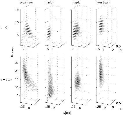
Figure 12: Estimates of joint probability density functions for the code features $\bar{\Delta},\bar{\alpha},n_{\Delta\geq 30\,\mathrm{\textrm{\textmu}s}}$ (see (6)). Top row: $\tau=0$; bottom row: $\tau=3\,\mathrm{ms}$. Estimates are based on $N=21\,200$ echoes each.

The suitability of the distances between the probability density functions for target classification was assessed by estimating performance measures of an m-ary sequential probability ratio test [23]. Because bats use pulse trains with repetition rates that are typically high compared to the time scales that navigation decisions are made on, this approach provides the necessary model to explain how bats could make use of the information which accumulates over the incoming echo trains.

The classification trials were conducted based on random draws of echoes from the stimulus ensemble, this discards any information which may be provided by systematic changes in echo features over a certain path [3]. Nevertheless, an excellent classification performance was found (Figure 13):

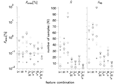
Figure 13: Classification trial results for the four foliage types based on the three distant cycle $\Delta\left(\alpha_{m},\alpha_{m+1}\right)$ features ($\bar{\Delta},\bar{\alpha},n_{\Delta\geq 30\,\mathrm{\textrm{\textmu}s}}$, see (6)) and their combinations. Left: estimated class conditional error probability [%]; center: expected number of samples (echoes) needed for a decision; right: 90%-percentile of the number of samples. Black symbols: $\tau=0$; gray symbols: $\tau=3\,\mathrm{ms}$. Responses of the spike coding model were drawn randomly from $21\,200$ examples for each class, $N=10^{5}$ trials were conducted for each performance estimate. See figure 6 for symbols denoting target class.

Using the joint probability density function of all three features and no smoothing ($\tau=0$), error probabilities of 0.03 to 0.19% were obtained on an expected number of 3 to 8 echoes (90%-percentiles ranged from 6 to 13). For moderate smoothing ($\tau=3\,\mathrm{ms}$), a slight performance decrease was found (error probabilities: 0.24 to 0.5%, expected number of samples: 5 to 8, 90%-percentiles: 9 to 13, see figure 13). Using the joint probability density function of all three features was found to result in the best overall performance, so both first order properties of the neural response as well as the number of time intervals contain target class information. Using all three features, the overall dependence of classification performance on preprocessing model parameters ($f_{c}$, $Q$, $\tau$) was found to be weak, average values (over all four target classes) of error probabilities, sample numbers and their 90%-percentiles were found to fall in the intervals 0.06-4.5%, 3-15 and 4-27 respectively. The least favorable values were outliers which were reached for a few, adverse parameter combinations only (Figure 14).

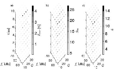
Figure 14: Dependence of classification performance on preprocessing model parameters. Parameters are: center frequency of the auditory bandpass channel model $f_{c}$, its $-3\,\mathrm{dB}$ filter quality $Q$, and smoothing time constant $\tau$. Performance measures are: a) Estimated classification error probability $\hat{P}_{\textrm{error}}$ (averaged over target class), b) 90%-percentile ($\hat{N}_{90}$) and c) expected value ($\bar{N}$) for the number of samples (echoes) needed for a decision.

These results demonstrate that the parameters of the preprocessing model are of little relevance within the parameter ranges ($f_{c}=\left[40\,\mathrm{kHz},65\,\mathrm{kHz}\right],Q=\left[10,35\right],\tau=\left[0,10\,\mathrm{ms}\right]$) studied.

6 Conclusions and directions for future research

The present work addresses the acoustic landmark identification as an example problem of biomimetic random process classification. Because the sensory representation of sound is low-dimensional, most biosonar sensing tasks involving extended, multi-faceted targets are likely to be posed in the way of random process estimation problems. In vision, this situation is much less common, because retinal images leave fewer alternative interpretations and often additional assumptions are available to decide between them. This leads to regularization approaches being considered as models of visual perception [24], which would fail in biosonar perception. The specific merit of biosonar as a sensory model system lies therefore in the fact that it matches vision in sustaining animals with active mobility in three-dimensional space despite this severe ill-posedness.

For the studied example problem, possible solutions were explored in a computational approach on a spike code level. The use of a parsimonious model for generating this spike code aides the search for basic, robust principles. Highly informative and accessible code features should be readily visible in the output of any model which reproduces the relevant principles correctly. The basic assumptions made here were the well-established view that spike-generation can be approximated as smoothing followed by thresholding and that time-differences are the elements of the code. The latter assumption is particularly appealing in bats, where small, monaural time differences are known to be behaviorally relevant as well as neurally extracted. In principle, however, the discovered features (extended troughs in the waveform) may as well be accessible in other codes, like e.g., a rate code. In bats, a rate code would have to be reconciled with the fact that signals of large bandwidth must be coded with a comparatively small number of auditory nerve fibers, which may result in excessively large estimator variance [25].

The interval code served as a biomimetic guide for identifying classification features. The central insight gained is that within all possible elementary interspike intervals (formed between neighboring thresholds) which an echo can generate, a few, comparatively long distant-cycle intervals stand out: They are readily resolved in isolation already and furthermore are the dominating component in any compound interspike interval (formed between distant thresholds) they are part of. Distant-cycle interspike intervals can be viewed as an acoustic analogue to edges in a visual image: They are the result of a discontinuity (in the inverse function of the waveform in the acoustic case) and are readily visible over a range of different resolutions (i.e., amplitude threshold spacings in the acoustic case). However, whereas in visual images edges tend to delineate the shape of deterministic objects or patterns, for echoes this not the case. Therefore, the problem of dealing with “echo edges” is not a pattern recognition problem, but a random process classification problem without a deterministic template.

The chosen example problem (classification of different foliages) holds little promise for classic feature selection methods: the probability density functions of signal amplitude are non-Gaussian [2], and the only non-negligible structure in the auto-covariance matrix is determined by the sonar pulse. Nevertheless the number, average duration and average amplitude location of the few distant-cycle interspike intervals in the spike response to each echo class were shown to provide excellent target class information. Therefore, the features which were found to be of high visibility in the spike code derived from a parsimonious model also proved to be highly informative.

Further work is needed to elucidate the structural basis of these features, i.e., what kind of physical target properties they correspond to. These could be the distributions of individual reflector properties (e.g., size, spatial orientation), properties of their spatial distribution or, more specifically, properties of the contours that limit these spatial distributions. In this way, the findings for the example stimulus ensemble considered here could be generalized to a more inclusive theory about the information that is accessible to biosonar systems in natural environments.

Finally, the coding model investigated has been limited to isolated portions (a single auditory bandpass channel) of the auditory signal representation and to random sequences of echoes. Relationships which may exist across the frequency dimension of the auditory signal representation [26] or across the echo sequence [3] generated along a particular flight path of a bat have been ignored. In the view of these omissions, the achieved classification performance is particularly remarkable. Using the full information available across frequency and scan path, bats may be able to make even finer discriminations (e.g., identifying different trees of the same species, different views or portions of the same tree). Spatial gradients explored along a flight path could be used for performing estimation tasks other than target classification, for instance, path planning, e.g., in the form of contour following, could be performed by following a spatial gradient in statistical echo properties. Assuming that the nature of such spatial gradients would depend on target class, research into the existence and information contend of spatial in the studied features would link target classification to a much wider set of tasks that animals need to perform in their natural habitats.

References

References

- [1] A. C. Kak and M. Slaney. Principles of Computerized Tomographic Imaging. Society for Industrial & Applied Mathematics, Philadelphia, 2001.
- [2] R. Müller and R. Kuc. Foliage echoes: a probe into the ecological acoustics of bat echolocation. J. Acoust. Soc. Am., 108(2):836–45, 2000.
- [3] Kuc R. Transforming echoes into pseudo-action potentials for classifying plants. J. Acoust. Soc. Am., 110(4):2198–206, Oct. 2001.
- [4] P. McKerrow and N. Harper. Plant acoustic density profile model of ctfm ultrasonic sensing. IEEE Sensors Journal, 1(4):245–55, Dec 2001.
- [5] Ö. Bozma and R. Kuc. Building a sonar map in a specular environment using a single mobile transducer. IEEE Trans. Pattern Analysis and Machine Intelligence, 13(12):1260–9, Dec 1991.
- [6] P. M. Morse and K. U. Ingard. Theoretical Acoustics. Princeton University Press, Princeton, New Jersey, 1986.
- [7] R. A. Suthers D. J. Hartley. The sound emission pattern of the echolocating bat, eptesicus fuscus. J. Acoust. Soc. Am., 85(3):1348–51, Mar 1989.
- [8] R.B. Coles, A. Guppy, M.E. Anderson, and P. Schlegel. Frequency sensitivity and directional hearing in the gleaning bat, plecotus auritus (Linnaeus 1758). J. Comp. Physiol. A, 165(2):269–80, 1989.
- [9] G. M. Jenkins and D. G. Watts. Spectral analysis and its applications. Holden-Day, Inc., San Francisco, 1968.
- [10] D. W. Scott. Multivariate Density Estimation. John Wiley & Sons, Inc., New York, 1992.
- [11] M. Slaney. An efficient implementation of the Patterson-Holdsworth auditory filter. Technical Report 35, Apple Computer, 1993.
- [12] T. Dau and D. Püschel. A quantitative model of the ”effective” signal processing in the auditory system. I. model structure. J. Acoust. Soc. Am., 99:3615–22, 1996.
- [13] R. Müller and H.-U. Schnitzler. Acoustic flow perception in cf-bats: extraction of parameters. J. Acoust. Soc. Am., 108(3):1298–307, 2000.
- [14] S. Haplea, E. Covey, and J.H. Casseday. Frequency tuning and response latencies at three levels in the brainstem of the echolocating bat, Eptesicus fuscus. J. Comp. Physiol. A, 174(6):671–83, Jun 1994.
- [15] P. Weissenbacher, L. Wiegrebe, and M. Kössl. The effect of preceding sonar emission on temporal integration in the bat, megaderma lyra. J. Comp. Physiol. A, 188(2):147–55, Mar 2002.
- [16] W. M. Kistler, W. Gerstner, and J. L. van Hemmen. Reduction of the Hodgkin-Huxley equations to a single-variable threshold model. Neural Computation, 9:1015–1045, 1997.
- [17] N. Kuwabara and N. Suga. Delay lines and amplitude selectivity are created in subthalamic auditory nuclei: the brachium of the inferior colliculus of the mustached bat. J. Neurophysiol., 69(5):1713–24, May 1993.
- [18] I. Saitoh and N. Suga. Long delay lines for ranging are created by inhibition in the inferior colliculus of the mustached bat. J. Neurophysiol., 74(1):1–11, Jul. 1995.
- [19] B. Grothe. The evolution of temporal processing in the medial superior olive, an auditory brainstem structure. Prog. Neurobiol., 61(6):581–610, Aug 2000.
- [20] M. Vater. Cochlear physiology and anatomy in bats. In P.E. Nachtigall and P.W.B. Moore, editors, Animal Sonar Processes and Performance, pages 225–42, New York, 1988. Plenum Press.
- [21] P. Heil and D. R. Irvine. First-spike timing of auditory-nerve fibers and comparison with auditory cortex. J. Neurophysiol., 78(5):2438–54, 1997.
- [22] C. Bourin and P. Bondon. Efficiency of higher order moment estimates. IEEE Transactions on Signal Processing, 46(1):255–8, Jan 1998.
- [23] C. W. Baum and V. V. Veeravalli. A sequential procedure for multihypothesis testing. IEEE Transactions on Information Theory, 40(6):1994–2007, 1994.
- [24] T. Poggio, V. Torre, and C. Koch. Computational vision and regularization theory. Nature, 317:314–9, 1985.
- [25] J. Gautrais and S. Thorpe. Rate coding versus temporal order coding: a theoretical approach. Biosystems, 48(1-3):57–65, Sep-Dec 1998.
- [26] L. S. Smith. Onset-based sound segmentation. In D.S. Touretzky, M.C. Mozer, and M.E. Hasselmo, editors, Advances in Neural Information Processing Systems 8 (Proceedings of the 1995 Conference), pages 729–35. MIT Press, 1996.