Improvement of experimental data via consistency conditions

Abstract

Interdependencies between experimental spectra, representing line or plane projections of electronic densities, are derived from their consistency and symmetry conditions. Some additional relations for plane projections are obtained by treating them as line projections of line projections.

The knowledge of these dependencies can be utilised both for an improvement of experimental data and for a verification of various techniques used for correcting e.g. two-dimensional (or one-dimensional) angular correlation of annihilation radiation spectra and Compton scattering profiles.

published in: Appl. Phys. A 70, 97-100 (2000)

I Introduction

All spectra, representing projections of the same density, must be interdependent. This so-called consistency condition (CC) has been considered for reconstructing densities $\rho({\bf p})$ from their line projections [1-3]. In the case of angular correlation of annihilation radiation ($ACAR$) spectra or Compton profiles (CP) measurements this condition is satisfied if spectra are measured up to such a momentum $p_{max}$ above which $\rho({\bf p})$ is isotropic and all projections have the same values.

The CC is automatically imposed on the experimental data via the reconstruction of $\rho({\bf p})$. However, it can be utilised for checking (before the reconstruction) if data were measured and next corrected (to remove various experimental imperfections) properly. Moreover, this condition can be also profitable for an improvement of such experimental data for which $\rho({\bf p})$ is not reconstructed. For this purpose one should estimate interdependences between projections what is a subject of this paper.

In the next Section we discuss the consistency condition in its general form, i.e. for the Radon transform in N-dimensional space. Next, some relations between line (Sec. II.A) and plane projections (Sec. II.B) are derived from both the CC and a symmetry of $\rho({\bf p})$ (electronic densisty in the momentum space) for various crystallographical structures. A fulfilment of these relations, proved for various model and experimental spectra, is discussed in Sec. III.

II Theory

The Radon transform [4] represents integrals of $\rho({\bf p})$ (defined in $N$-dimensional space, ${\cal R}^{N}$) over $(N-1)$-dimensional hyperplanes:

$$\hat{R}\cdot\rho({\bf p})=g(t,\mbox{\boldmath$\zeta$})=\int_{-\infty}^{\infty}\rho({\bf p})\delta(t-\mbox{\boldmath$\zeta$}\cdot{\bf p})d{\bf p},$$ (1)

where $\zeta$ is a unit vector in ${\cal R}^{N}$ along $t$ and $t$ is a perpendicular distance of the hyperplane from the origin of the coordinate system. The equation $t=\mbox{\boldmath$\zeta$}\cdot{\bf p}$ defines the hyperplane. In the same coordinate system the vector ${\bf p}$ is described by $p=|{\bf p}|$ and $\omega$ (e.g. Dean [5]).

Both functions, $g$ and $\rho$, can be expanded into spherical harmonics of degree $l$:

$$g(t,\mbox{\boldmath$\zeta$})=\sum_{l\nu}g_{l\nu}(t)S_{l\nu}(\mbox{\boldmath$\zeta$}),$$ (2)

$$\rho(p,\mbox{\boldmath$\omega$})=\sum_{l\nu}\rho_{l\nu}(p)S_{l\nu}(\mbox{\boldmath$\omega$}),$$ (3)

where index $\nu$ distinguishes harmonics of the same order $l$. In order to make our formuale clearer, henceforth index $\nu$ will be omitted, keeping in mind that for the same $l$ a few harmonics can be used. According to Dean [5],

$$\rho_{l}(p)=\frac{c}{p}\int_{p}^{\infty}g_{l}^{(2\mu+1)}(t)C_{l}^{\mu}(t/p)[(t/p)^{2}-1]^{\mu-1/2}dt,$$ (4)

where $c=(-1)^{2\mu+1}\Gamma(l+1)\Gamma(\mu)/(2\pi^{\mu+1}\Gamma(l+2\mu))$. Here $g^{(n)}$ denotes the $n^{th}$ derivative of $g$ ; $C^{\mu}_{l}$ are Gegenbauer polynomials and $\mu=N/2-1$. The equation (4) can be solved analitically if either [6]

$$g_{l}(t)=\sum^{\infty}_{k=0}a_{lk}(1-t^{2})^{\lambda-1/2}C^{\lambda}_{l+2k}(t),$$ (5)

with $\lambda>N/2-1$, or [7]

$$g_{l}(t)=e^{-t^{2}}\sum^{\infty}_{k=0}b_{lk}H_{l+2k}(t),$$ (6)

where $H_{m}$ are the Hermite polynomials. Because in $\rho_{l}(p)$ all terms $t^{n}$ with $0\leq n<l$ are equal to zero, the lowest term in $g_{l}$ is of order $l$. This property, called CC, follows from the fact that functions $g_{l}$ (Eq. (2)) are a linear combination of $g(t,\mbox{\boldmath$\zeta$})$ which in turn are interdependent being projections of the same density. Generally, one can write

$$g_{l}(t)=\sum^{\infty}_{k=0}c_{lk}W_{l+2k}(t),$$ (7)

where $W_{n}$ denotes an arbitrary orthogonal polynomial. Below, considering the cases $N=2$ (line projections) and $N=3$ (plane projections), we show that due to this property of $g_{l}(t)$ (its minimal number of zeros) we can get some interdependences between projections $g(t,\mbox{\boldmath$\zeta$})$. For that it is necessary to expand them into a series of the same (as in Eq. (7)) polynomials:

$$g(t,\mbox{\boldmath$\zeta$})=\sum^{\infty}_{k=0}c_{k}(\zeta)W_{2k}(t).$$ (8)

By combining Eqs. (2), (7) and (8) we can obtain some relations between $c_{k}(\zeta)$ as a function of $\zeta$. In the paper, for calculating the coefficients $c_{k}$, the Chebyshev polynomials and the Gaussian quadrature formulae were applied.

II.1 Line projections

In the case of reconstructing $\rho({\bf p})$ from its line projections $g(x,y)$ (measured in the apparatus systems $(x,y,z)$), the reconstruction of the three–dimensional ($3D$) density can be reduced to a set of reconstructions of $2D$ densities (the Radon transform for $N=2$) performed, independently, on succeeding planes $y=const.$, parallel each other. In order to describe all projections in the same coordinate system (in which the symmetry of both $\rho({\bf p})$ and measured spectra is defined) the function $g$ can be characterized in the polar system where $g(x,y)\equiv g(t,\alpha)$. Here $t$ and $\alpha$ denote the distance of the integration line from the origin of the coordinate system and its angle with respect to a chosen axis, respectively.

For the planes $y=const.$, perpendicular to the axis of the crystal rotation of the order $|G|$, Eq. (2) reduces to the $cosine$ series [8]:

$$g(t,\alpha)=\sum_{l}^{\infty}g_{l}(t)\cos(l\alpha),$$ (9)

with $l=i\cdot|G|$ ($l=0$, $|G|$, $2|G|$, etc.). Here the angle $\alpha$, describing nonequivalent directions, is changing between $0\leq\alpha\leq\alpha_{G}=\pi/|G|$. Of course, to use the symmetry most profitably, a sensible choice is to select the planes perpendicular to the main axis of the crystal rotation ($|G|=4$ or $6$ for cubic and tetragonal or hexagonal structures, respectively) where $\alpha_{G}$ is minimal, i.e. the number of equivalent directions is maximal.

Knowing that $l/2$ first coefficients $c_{lk}$ are equal to zero (Eq. (7)), the equations (8) and (9) give the following dependences between $c_{k}(\alpha)$

$1^{0}.$

$c_{k}(\alpha)=c_{0k}$, i.e. $|G|/2$ first coefficients $c_{k}(\alpha)$ are the same for all projections.

$2^{0}.$

$2c_{k}(\alpha_{G}/2)=c_{k}(\alpha)+c_{k}(\alpha_{G}-\alpha)$ for $k\leq|G|$.

$3^{0}$.

$2\{c_{k}(\alpha_{G}/4)+c_{k}(3\alpha_{G}/4)\}=c_{k}(\alpha)+c_{k}(\alpha_{G}/2-\alpha)+c_{k}(\alpha_{G}/2+\alpha)+c_{k}(\alpha_{G}-\alpha)$ for $k\leq 2|G|$.

All these conditions have been proved for both various models of $\rho({\bf p})$ and for $|G|=2$, $4$ and $6$.

II.2 Plane projections

Due to the symmetry of $\rho({\bf p})$, in the case of $N=3$, $g(t,\mbox{\boldmath$\zeta$})\equiv g(t,\Theta,\varphi)$ can be expanded into the lattice harmonics $F_{l}(\Theta,\varphi)$ which form an orthogonal set of linear combinations of the spherical harmonics $K^{m}_{l}=c(l,m)P^{|m|}_{l}(\cos\Theta)(e^{im\varphi}+e^{-im\varphi})$. $c(l,m)$ is the normalization constant and $P^{|m|}_{l}(\cos\Theta)$ denotes the associated Legendre polynomial. Angles $(\Theta,\varphi)$ describe the azimuthal and the polar angles of the $\zeta$-axis with respect to the reciprocal lattice system.

In the case of the hexagonal structure $F_{l}=K_{l}^{m}$ with $l=0$ $mod$ $2$ and $m=0$ $mod$ $6$ ($K_{0}^{0}=1$, $K_{2}^{0}$, $K_{4}^{0}$, $K_{6}^{0}$, $K_{6}^{6}$, $K_{8}^{0}$, $K_{8}^{6}$, etc.), for the tetragonal structure $F_{l}=K_{l}^{m}$ with $l=0$ $mod$ $2$ and $m=0$ $mod$ $4$ and for the cubic structures $F_{l}$ are the linear combinations of $K_{l}^{m}$, where the first three are equal to [9]:

$F_{0}=1$,

$F_{4}=0.76376261K_{4}^{0}+0.64549722K_{4}^{4}$,

$F_{6}=0.35355338K_{6}^{0}-0.9354134K_{6}^{4}$.

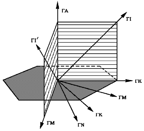
Figure 1: Planes and directions for the hexagonal structure having symmetry of the sixth and the second order, marked by dots and lines, respectively.

So, for the hexagonal and tetragonal structures a few first lattice harmonics do not depend on $\varphi$. Moreover, very often, for some paticular sets of measured spectra, we cannot calculate functions $g_{l}(t)$ (the matrix in Eq. (2) is singular). For example: if for the hexagonal structure we have only three projections with $\zeta$ along the $\Gamma M$, $\Gamma K$ and $\Gamma A$ symmetry directions (Fig. 1), the angles $(\Theta,\varphi)$ are equal to: $(\pi/2,\pi/6)$, $(\pi/2,0)$ and $(0,0)$, respectively. Thus, the first three lattice harmonics have the same values for the $\Gamma M$ and $\Gamma K$ directions and there is no a possibility to evaluate functions $g_{l}(t)$. Next, if e.g. $(\Theta,\varphi)=(0,0)$, $(\pi/4,0)$, $(\pi/2,0)$, $(\pi/4,\pi/6)$, $(\pi/2,\pi/6)$, the set of equations for $g_{l}$ does not have a solution in spite of the fact that the first five harmonics distinguish here all directions $\zeta$. Due to these reasons we propose to treat plane projections of $\rho({\bf p})$ as line projections of $\tilde{\rho}_{L}$ and to use the consistency and symmetry conditions derived in Sec. II.A.

We consider only those spectra $g(t,\mbox{\boldmath$\zeta$})$ for which $\zeta$ is changed on the plane perpendicular to the axis of the crystal rotation of the order $|G|$. In such a case $\tilde{\rho}_{L}$ denotes the line integral of $\rho({\bf p})$ along lines $L$ parallel to this axis and $g(t,\mbox{\boldmath$\zeta$})$ can be described by Eq.(9). Now all relations obtained for the line projections are valid with $c_{k}(\alpha)$ being replaced by $c_{k}(\mbox{\boldmath$\zeta$})\equiv c_{k}(\Theta,\varphi)$ where either $\alpha=\varphi$ and $\Theta=\pi/2$ (for the planes perpendicular to the main axis of the crystal rotation) or $\alpha=\Theta$ and $\varphi=const.$ (for the planes with $|G|=2$, perpendicular to the previous ones).

For example, for three spectra having the hexagonal symmetry and with $\zeta$ along the $\Gamma M$, $\Gamma K$ and $\Gamma A$ symmetry directions (denoted here by $g(\Gamma M)$, $g(\Gamma K)$ and $g(\Gamma A)$) we have the following relations: $c_{k}(\Gamma M)=c_{k}(\Gamma K)$ for $k=0$, $1$, $2$ (here $|G|=6$) and $c_{0}(\Gamma A)=c_{0}(\Gamma M)=c_{0}(\Gamma K)$ ($|G|=2$), where $c_{0}$ denotes the norm of the spectrum. So, to get more information about $g(\Gamma A)$ we should have at least one additional spectrum $g(\Gamma I)$ (for $\Theta=\pi/4$ and e.g. $\varphi=0$) on the plane with $|G|=2$ where $2c_{1}(\Gamma I)=c_{1}(\Gamma A)+c_{1}(\Gamma K)$ (see Fig. 1). This equality is satisfied for $\Theta=\pi/4$ and any $\varphi\in(0,\pi/6)$, i.e. $2c_{1}(\Gamma I^{\prime\prime})=c_{1}(\Gamma A)+c_{1}(\Gamma N)$, where the $\Gamma N$ and $\Gamma I^{\prime\prime}$ directions are defined by the same $\varphi$ with $\Theta=\pi/2$ and $\Theta=\pi/4$, respectively. Knowing that $c_{1}(\Gamma N)=c_{1}$ (does not depend on $\varphi$) we obtain that $c_{1}(\Theta=\pi/4,\varphi)$ has the same value for each spectrum $g(\mbox{\boldmath$\zeta$})$ with $\zeta$ described by $\Theta=\pi/4$ and any $\varphi$. This is derived by treating $g(\Gamma N)$ simultaneously as the line projection of $\tilde{\rho}_{|6|}$ and $\tilde{\rho}_{|2|}$ with the symmetry $|G|=6$ and $|G|=2$, respectively. Here $\tilde{\rho}_{|6|}$ represents the line projection of $\rho({\bf p})$ along the main axis of the rotation, while $\tilde{\rho}_{|2|}$ along any line perpendicular to this axis. This last dependence is particularly interesting because it gives interdependence between line projections of different densities, while all consistency conditions for the line projections are for the same $\tilde{\rho}$.

All dependencies, shown here on the example of the hexagonal structure, are valid for the cubic and tetragonal structures where $|G|=6$ is replaced by $|G|=4$. However, for the cubic structures, where three axes of the fourth order exist, one can get some additional rules. Because directions $(\Theta,\varphi)=(0,0)$ and $(\pi/2,0)$ are equivalent, we obtain that not only $c_{0}$ but also $c_{1}$ must be the same for all projections. Some of these results can be also derived from Eq. (2) because for the cubic structures all lattice harmonics (except for $F_{0}$) depend on $(\Theta,\varphi)$. Taking as an example directions $[00h]$, $[kl0]$ and $[klh]$ we obtain the following dependences between $c_{i}$:

$a_{1}c_{i}([00h])+a_{2}c_{i}([kl0])+a_{3}c_{i}([klh])=0$ for $i=0,1$

$b_{1}c_{i}([00h])+b_{2}c_{i}([kl0])+b_{3}c_{i}([klh])=0$ for $i=0,1,2$ where $\sum b_{i}=\sum a_{i}=0$.

The above equalities arise from the conditions of vanishing all polynomials $W_{i}$ with $i=0,1$ and $i=0,1,2$ in the expansion of $g_{4}(t)$ and $g_{6}(t)$, respectively. The coefficient $c_{1}$ satisfies both equations when $c_{1}([00h])=c_{1}([kl0])=c_{1}([klh])$ what is in agreement with the previous result. Knowing additionally that $c_{1}([kl0])$ does not depend on the direction $[kl0]$, we can conclude that for the cubic structure the value of $c_{1}([klh]$) does not depend on the direction (denoted here by $[klh]$).

As before, all relations were proved for both model and experimental profiles. Some examples are presented in the next section.

III Application

First, disposing twenty five $2D$ $ACAR$ experimental spectra [10] for the four metals of the hcp structure with $\zeta$ on the plane $|G|=6$, we obtained that the conditions $1^{0}$ and $2^{0}$ are satisfied with a very high accuracy, lower than $0.5\%$ ($c_{1}$), $1.5\%$ ($c_{2}$), $1.5\%$ ($c_{3}$), $2.5\%$ ($c_{4}$) and $5.5\%$ ($c_{5}$). Because the first $ck{m}(\mbox{\boldmath$\zeta$})$ have the highest values, they are determined the best (the influence of the statistical noise is the lowest). This very small inconsistency implies that spectra [10] (with the average number of counts at peak about 60000) were not only measured but also corrected with a very high precision.

In the figure 2 we show results for the theoretical Compton profiles for Cr [11] with $\zeta$ along $[100]$, $[110]$ and $[111]$ directions. In this case (cubic structure) the first two coefficients $c_{k}(\mbox{\boldmath$\zeta$})$ should have the same value for each spectrum, while the third coefficient should satisfy the relation: $c[100]-c[110]=3\{c[110]-c[111]\}$. After normalizing spectra to the same area ($c_{0}=1$) we obtained that a distortion of $c_{1}$ from its average value is changed from $0.1\%$ up to $0.4\%$ and the inconsistency of $c_{2}$ is of order $1.5\%$. Thus, the behaviour of $c_{k}(\mbox{\boldmath$\zeta$})$ is the same as for previously studied experimental data. It is connected with the fact that in order to create such spectra it would be necessary to calculate $\rho({\bf p})$ in the whole momentum space ${\bf p}$, what, of course, cannot be done. Here the accuracy of calculating Compton profiles was comparable with the statistical noise of 2D ACAR data [10]. Of course, in order to get the similar inconsistency of the Compton profiles (where a contribution of core densities is much higher than in a positron annihilation experiment) the experimental statistic must be also much higher.

In order to examine how these conditions react to an improper shape of $g(t,\mbox{\boldmath$\zeta$})$, we changed somewhat the shape of one spectrum ( marked in figure 2 by squares). Here we would like to point out that this incorrect spectrum does not differ from other spectra too much (the differences between $g([100])$ and $g([111])$ are higher). After normalizing it to the same area ($c_{0}=1$) we obtained that $c_{1}$ changed its value from -0.7 to -0.74 . So, here we observe a much higher inconsistency ($5\%$) than for experimental data [10] ($0.5\%$).

IV Conclusions

All spectra received from experiments are contaminated by statistical noise and thus they are not consistent. Depending on the number of measured projections, some part of the inconsistent noise is eliminated via the consistency conditions during the reconstruction of $\rho({\bf p})$. However, we propose to check (before the reconstruction) if spectra were measured and corrected properly (the inconsistent part of the data cannot be too large). For that purpose we can use the interdependences, derived by combining the consistency and symmetry conditions, obtained here for the line and plane projections.

The knowledge of the interdependences rules can be also profitable for an improvement of data for which densities are not reconstructed (some part of the inconsistent noise can be eliminated). Moreover, it can be applied to verify these techniques which are used for correcting Compton scattering spectra (they are not univocal and can be individual for each spectrum [12]). For that we propose to measure the high resolution CP, denoted usually by $J(p_{z})$, for hexagonal metals with $p_{z}\equiv\mbox{\boldmath$\zeta$}$ changed on the plane $|G|=6$ ($\Theta=\pi/2$). Having $p_{z}$ along $\Gamma K$ ($\varphi=0$), $\Gamma M$ ($\varphi=\pi/6$) and $\Gamma N$ ($\varphi=\pi/12$), we can check if $c_{i}(\Gamma K)=c_{i}(\Gamma M)=c_{i}(\Gamma N)$ for $i=0,1,2$ and if $c_{i}(\Gamma K)+c_{i}(\Gamma M)=2c_{i}(\Gamma N)$ for $i=3,4,5$. Of course, the best choice is to study rare-earth metals where the anisotropy of $\rho({\bf p})$ is so high that spectra $J(p_{z})$ should be essentionally different.

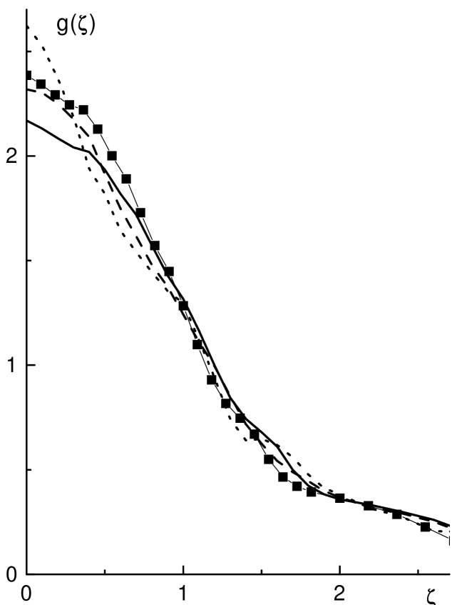
Figure 2: Theoretical plane projections for Cr [11] having cubic symmetry with ${\bf\zeta}$ along [100], [110] and [111] directions marked by full, broken and dotted lines, respectivelly. Incorrect projection [110] is marked by the full squares.

References

- (1) A. M. Cormack, J. Appl. Phys., 35, 2908 (1964).
- (2) R. M. Lewitt, Proc. IEEE, 71, 390 (1983); (b) R. M. Lewitt and R. H. T. Bates, Optik, 50, 189 (1978).
- (3) H. Kudo and T. Saito, J. Opt. Soc. Am., A 8, 1148 (1991).
- (4) J. Radon Ber. Verh. Sachs. Akad., 69, 262 (1917).
- (5) The Radon Transform and Some of Its Applications, S. R. Dean, John Wiley and Sons, NY-Chichester-Brisbane-Toronto-Singapore 1983.
- (6) A. K. Luis, SIAM J. Math. Anal., 15, 621 (1984).
- (7) A. M. Cormack, Proc. American Math. Society, 86, 293 (1982).
- (8) G. Kontrym-Sznajd, Phys. Stat. Solidi (a), 117, 227 (1990).
- (9) F. M. Mueller and M. G. Priestley, Phys. Rev. 148, 638 (1966).
- (10) P. A. Walters, J. Mayers and R. N. West, Positron Annihilation, eds. P. G. Coleman et. al., North-Holland Publ. Co., 1982, p. 334; R. L. Waspe and R. N. West, ibid., p. 328; A. Alam, R. L. Waspe and R. N. West, Positron Annihilation, eds. L. Dorikens-Vanpraet et al., World Sci., Singapore 1988, p. 242; S. B. Dugdale, H. M. Fretwell, M. A. Alam, G. Kontrym-Sznajd, R. N.West and S. Badrzadeh, Phys. Rev. Lett., 79, 941 (1997).
- (11) Handbook of calculated electron momentum distributions, Compton profiles and X-ray factors of elemental solids, N. I. Papanicolaou, N. C. Bacalis and D. A. Papaconstantopoulos, CRC Press, Boca Raton 1991.
- (12) L. Dobrzyński, private communication.