The Coupled Electronic-Ionic Monte Carlo Simulation Method

Abstract

Quantum Monte Carlo (QMC) methods such as Variational Monte Carlo, Diffusion Monte Carlo or Path Integral Monte Carlo are the most accurate and general methods for computing total electronic energies. We will review methods we have developed to perform QMC for the electrons coupled to a classical Monte Carlo simulation of the ions. In this method, one estimates the Born-Oppenheimer energy $E(Z)$ where $Z$ represents the ionic degrees of freedom. That estimate of the energy is used in a Metropolis simulation of the ionic degrees of freedom. Important aspects of this method are how to deal with the noise, which QMC method and which trial function to use, how to deal with generalized boundary conditions on the wave function so as to reduce the finite size effects. We discuss some advantages of the CEIMC method concerning how the quantum effects of the ionic degrees of freedom can be included and how the boundary conditions can be integrated over. Using these methods, we have performed simulations of liquid H₂ and metallic H on a parallel computer.

1 Introduction

The first computer simulations of a condensed matter system used the simplest inter-atomic potential, the hard sphere interactionmetropolis53 . As computers and simulation methods progressed, more sophisticated and realistic potentials came into use, for example the Lennard–Jones potential to describe rare gas systems, the potential functions being parameterized and then fit to reproduce experimental quantities. Both Molecular Dynamics (MD) and Monte Carlo (MC) methods can be used to generate ensemble averages of many-particle systems, MC being simpler and only useful for equilibrium properties.

Inter–atomic potentials originate from the microscopic structure of matter, described in terms of electrons, nuclei, and the Schrödinger equation. But the many-body Schrödinger equation is too difficult to solve directly, so approximations are needed. In practice, one usually makes the one electron approximation, where a single electron interacts with the potential due to the nuclear charge and with the mean electric field generated by all the other electrons. This is done by Hartree–Fock (HF) or with Density Functional Theory (DFT)parr89 . DFT is, in principle, exact, but contains an unknown exchange and correlation functional that must be approximated, the most simplest being the Local Density Approximation (LDA) but various improvements are also used.

In 1985, Car and Parrinello introduced their method, which replaced an assumed functional form for the potential with a LDA-DFT calculation done “on the fly”car85 . They did a molecular dynamics simulation of the nuclei of liquid silicon by computing the density functional forces of the electronic degrees of freedom at every MD step. It has been a very successful method, with the original paper being cited thousands of times since its publication. There are many applications and extensions of the Car–Parrinello methodpayne92 ; marx96 ; sprik00 ; tuckerman00 . The review of applications to liquid state problems by Spriksprik00 notes that the LDA approximation is not sufficient for an accurate simulation of water although there are improved functionals that are much more accurate.

Quantum Monte Carlo (QMC) methods have developed as another means for accurately solving the many body Schrödinger equationfoulkes ; hammond94 ; anderson95 ; ceperley96 . The success of QMC is due largely to the explicit representation of electrons as particles, so that the electronic exchange and correlation effects can be directly treated. Particularly within the LDA, DFT has known difficulties in handling electron correlationgrossman95 .

In the spirit of the Car-Parrinello method, in this paper we describe initial attempts to combine a Classical Monte Carlo simulation of the nuclei with a QMC simulation for the electrons. This we call Coupled Electronic-Ionic Monte Carlo (CEIMC)dewing00b . As an example of this new method we apply it to warm dense many-body hydrogen. Hydrogen is the most abundant element in the universe, making an understanding of its properties important, particularly for astrophysical applications. Models of the interiors of the giant planets depends on a knowledge of the equation of state of hydrogenhubbard84 ; stevenson88 . Hydrogen is also the simplest element, but it still displays remarkable variety in its properties and phase diagram. It has several solid phases at low temperature, and the crystal structure of one of them (phase III) is not fully known yet. At high temperature and pressure the fluid becomes metallic, but the exact nature of the transition is not known, nor is the melting transition from liquid to solid for pressures above 1 MBar. The present knowledge of the phase diagram of hydrogen is summarized in Figure 1.

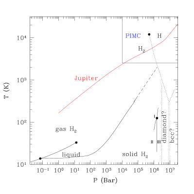
Figure 1: Phase Diagram of hydrogen. Solid lines are experimental determination, dashed line are theoretical estimates. Red curves show estimates of slices through the giant planets. The box shows roughly the domain of applicability of PIMC.

Some of the previous QMC calculations have been at high temperature using the restricted Path Integral MC method. This method becomes computationally inefficient at temperatures a factor of ten lower than the Fermi temperaturemilitzer00a . At the present time it is not known how to make the PIMC method efficient at the low temperatures needed to calculate interesting portions of the phase diagram. Zero temperature QMC methods have been used for calculations in the ground stateca87 ; natoli93 ; natoli95 with full quantum effects used for both the electronic and protonic degrees of freedom. In such cases it is hard to ensure that the protonic degrees of freedom are fully converged because of the problem that the electron and protons require two different time scales which differ by three orders of magnitude. In addition, finite temperature effects of the protons are beyond the reach of the method. CEIMC provides a middle way : the electrons are at zero temperature where accurate trial functions are known and the zero variance principle applies, while the protons (either classical or quantum) are at finite temperature and not subjected to the limitations imposed by the electronic time scale.

The electrons are assumed to be in their ground state, both in the Car–Parrinello method and in CEIMC. There are two internal effects that could excite the electrons, namely coupling to nuclear motion and thermal excitations. In the first case, we make the Born–Oppenheimer approximation, where the nuclei are so much more massive than the electrons that the electrons are assumed to respond to nuclear motion instantaneously, and so stay in their ground state. We neglect any occupation of excited states of the electrons due to coupling to nuclear motion. To estimate the effect of thermal excitation in metallic hydrogen, consider a gas of degenerate electrons at a density of $n=0.0298$ electrons per cubic Bohr (i.e. $r_{s}=\left(4\pi n/3\right)^{-1/3}=2.0$). This has a Fermi temperature of about 140,000 K. In the molecular hydrogen phase, the gap between the ground state and the first excited state of a hydrogen molecule at the equilibrium bond distance is about 124,000 K. Since our temperatures are well below this, and we are not at too high pressures (since the pressure decreases the gap), the thermal occupation of excited states can be neglected. At higher pressure however, when the electrons becomes delocalized and the system becomes metallic thermal effects can be relevant.

This report brings up-to-date previous work on CEIMC described in ref. dewing . The rest of this paper is as follows. First, we will describe the penalty method to rigorously deal with the noisy QMC estimates of energy differences. Then we will briefly discuss method for computing energy differences. Next, the choice of trial wave function will be discussed. Finally, we put all the pieces of a CEIMC simulation together and discuss preliminary results appropriate to many-body hydrogen.

2 The Coupled Electronic-Ionic Monte Carlo Method

First let us recall the basic ideas of Variational Monte Carlo (VMC) and Diffusion Monte Carlo. VMC uses the Metropolis method to sample the ratio of integrals and gives an upper bound to the exact ground state energy.

$$E=\frac{\int dR\left|\psi_{T}(R)\right|^{2}E_{L}(R)}{\int dR\left|\psi_{T}(R)\right|^{2}}$$ (1)

where $E_{L}=(H\psi_{T})/\psi_{T}$ is the local energy. Important features of VMC are that any computable trial function can be used for $\psi_{T}$ and that the statistical uncertainty vanishes as $\psi_{T}$ approaches an exact eigenstate.

The second QMC method we apply is diffusion Monte Carlo (DMC) in which the Hamiltonian is applied to the VMC distribution to project out the ground state:

$$\phi(t)=\psi_{T}\mathrm{e}^{-(H-E_{T})t}\phi(0)/\psi_{T}.$$ (2)

The VMC method, though it can directly include correlation effects, is not sufficiently accurate, at relevant temperatures, as we discuss below. The projection is implemented by a branching, drifting random walkreynolds82 though there are some advantages to working in a time independent framework of ground state path integrals. To maintain a positive function, needed for efficient sampling, the fixed-node approximation is used. Though an uncontrolled approximation, estimates of the resulting error lead to the conclusionfoulkes that the systematic error of this approximation are small, especially when accurate nodal surfaces are used.

In the CEIMC method we move the protons with a “classical” Monte Carlo and accept or reject to satisfy detailed balance. The Metropolis acceptance formula is

$$A=\min\left[1,\exp(-\Delta)\right]$$ (3)

where $\Delta=\beta[V(s^{\prime})-V(s)]$ and $V(s)$ is the BO electronic energy, computed with one of the QMC methods. The QMC simulation will yield a noisy estimate for $\Delta$, which we denote as $\delta$. The exponential in the acceptance ratio is nonlinear, so that $\langle\exp(-\delta)\rangle\neq\exp(\langle-\delta\rangle)$. The noise will introduce a bias into our acceptance ratio formula. Such bias is unacceptable since the main motivation for the CEIMC method is to improve the accuracy beyond what can be achieved with alternative approaches. To avoid this bias in our simulations, we can either run until the noise is negligible, but that is very time-consuming, or we can use the penalty methodceperley99 which tolerates noise. We describe this method next.

3 The Penalty Method

The basis of the penalty method is to satisfy detailed balance on average by using information about the energy differences. We introduce the “instantaneous” acceptance probability, $a(\delta)$, which is a function of the estimated energy difference. The average acceptance probability is the acceptance probability averaged over the noise,

$$A(s\rightarrow s^{\prime})=\int_{-\infty}^{\infty}d\delta P(\delta;s\rightarrow s^{\prime})a(\delta).$$ (4)

We need to satisfy detailed balance on average,

$$A(s\rightarrow s^{\prime})=A(s^{\prime}\rightarrow s)\exp\left[-\Delta\right]$$ (5)

If the noise is normally distributed with variance, $\sigma$, it has the distribution

$$P(\delta)=(2\sigma^{2}\pi)^{-1/2}\exp\left[-\frac{(\delta-\Delta)^{2}}{2\sigma^{2}}\right].$$ (6)

Then a simple solution that satisfies average detailed balance is

$$a(\delta)=\min\left[1,\exp(-\delta-\frac{\sigma^{2}}{2})\right]$$ (7)

The extra $-\sigma^{2}/2$ term causes additional rejections of trial moves due to noise. For this reason, it is called the penalty method.

An important issue is to verify that the energy differences are normally distributed. Recall that if moments of the energy are bounded, the central limit theorem implies that given enough samples, the distribution of the mean value will be Gaussian. Careful attention to the trial function to ensure that the local energies are well behaved may be needed.

In practice, the variance is also estimated from the data, and a similar process leads to additional penalty terms. Let $\chi$ be the estimate for $\sigma$ using $n$ samples. Then the instantaneous acceptance probability is

$$a(\delta,\chi^{2},n)=\min\left[1,\exp(-\delta-u_{B})\right]$$ (8)

where

$$u_{B}=\frac{\chi^{2}}{2}+\frac{\chi^{4}}{4(n+1)}+\frac{\chi^{6}}{3(n+1)(n+3)}+\cdots$$ (9)

Note that as the number of independent samples $n$ gets large, the first term dominates.

The noise level of a system can be characterized by the relative noise parameter, $f=(\beta\sigma)^{2}t/t_{0}$, where $t$ is the computer time spent reducing the noise, and $t_{0}$ is the computer time spent on other pursuits, such as optimizing the VMC wave function or equilibrating the DMC runs. A small $f$ means little time is being spent on reducing noise, where a large $f$ means much time is being spent reducing noise. For a double well potential, the noise level that gives the maximum efficiency is around $\beta\sigma\approx 1$, with the optimal noise level increasing as the relative noise parameter increases ceperley99 .

We can use multi–level sampling to make CEIMC more efficient ceperley95 . An empirical potential is used to “pre-reject” moves that would cause particles to overlap and be rejected anyway. A trial move is proposed and accepted or rejected based on a classical potential

$$A_{1}=\min\left[1,\frac{T(R\rightarrow R^{\prime})}{T(R^{\prime}\rightarrow R)}\exp(-\beta\Delta V_{cl})\right]$$ (10)

where $\Delta V_{cl}=V_{cl}(R^{\prime})-V_{cl}(R)$ and $T$ is the sampling probability for a move. If it is accepted at this first level, the QMC energy difference is computed and accepted with probability

$$A_{2}=\min\left[1,\exp(-\beta\Delta V_{QMC}-u_{B})\exp(\beta\Delta V_{cl})\right]$$ (11)

where $u_{B}$ is the noise penalty.

Compared to the cost of evaluating the QMC energy difference, computing the classical energy difference is much less expensive. Reducing the number of QMC energy difference evaluations reduces the overall computer time required. For the molecular hydrogen system, using the pre–rejection technique with a CEIMC–DMC simulation results in a first level (classical potential) acceptance ratio of 0.43, and a second level (quantum potential) acceptance ratio of 0.52. The penalty method rejects additional trial moves because of noise. If these rejections are counted as acceptances (i.e., no penalty method or no noise), then the second level acceptance ratio would be 0.71.

4 Energy Differences

In Monte Carlo it is the energy difference between an old position and a trial position that is needed. Using correlated sampling methods it is possible to compute the energy difference with a smaller statistical error than each individual energy. We also need to ensure that that energy difference is unbiased and normally distributed. In this section we briefly discuss several methods for computing that difference.

4.1 Direct Difference

The most straightforward method for computing the difference in energy between two systems is to perform independent computations for the energy of each system. Then the energy difference and error estimate are given by

$$\Delta E = E_{1}-E_{2}$$ (12)

$$\sigma(\Delta E) = \sqrt{\sigma_{1}^{2}+\sigma_{2}^{2}}$$ (13)

This method is simple and robust, but has the drawback that the error is related to the error in computing a single system. If the nuclear positions are close together, the energy difference is likely to be small and difficult to resolve, since $\sigma_{1}$ and $\sigma_{2}$ are determined by the entire system. Hence the computation time is proportional to the size of the system, not to how far the ions are moved.

4.2 Reweighting

Reweighting is the simplest correlated sampling method. The same set of sample points, obtained by sampling $p(R)\propto\psi_{1}^{2}$ is used for evaluating both energies. The energy difference is estimated as:

$$\Delta E = E_{1}-E_{2}$$ (14)

$$= \frac{\int dR\ \psi_{1}^{2}\ E_{L1}}{\int dR\ \psi_{1}^{2}}-\frac{\int dR\ \psi_{2}^{2}\ E_{L2}}{\int dR\ \psi_{2}^{2}}$$ (15)

$$= \frac{\int dR\ p(R)\left(\frac{\psi_{1}^{2}}{p(R)}\right)\ E_{L1}}{\int dR\ p(R)\left(\frac{\psi_{1}^{2}}{p(R)}\right)}-\frac{\int dR\ p(R)\left(\frac{\psi_{2}^{2}}{p(R)}\right)\ E_{L2}}{\int dR\ p(R)\ \left(\frac{\psi_{2}^{2}}{p(R)}\right).}$$ (16)

Then an estimate of $\Delta E$ for a finite simulation is

$$\Delta E\approx\sum_{R_{i}\in\psi^{2}_{1}}\left[\frac{E_{L1}(R_{i})}{N}-\frac{w(R_{i})E_{L2}(R_{i})}{\sum_{i}w(R_{i})}\right]$$ (17)

where $w=\psi_{2}^{2}/p(R)$.

Reweighting works well when $\psi_{1}$ and $\psi_{2}$ are not too different, and thus have large overlap. As the overlap between them decreases, reweighting gets worse due to large fluctuations in the weights. Eventually, one or a few large weights will come to dominate the sum, the variance in $\Delta E$ will be larger than that of the direct method. In addition, the distribution of energy differences will be less normal.

4.3 Importance Sampling

In dewing we discussed two-sided sampling: the advantages of sampling the points in a symmetrical way. Here we introduce a similar method, namely the use of importance sampling to compute the energy difference. Importance sampling is conceptually similar to the reweighting described above, however, we optimize the sampling function $p(r)$ so as to minimize the variance of the energy difference. If we neglect sequential correlation caused by the Markov sampling, it is straightforward to determine the optimal function:

$$p^{*}(R)\propto|\psi_{1}^{2}(R)(E_{L1}(R)-E_{1})-Q\psi_{2}^{2}(R)(E_{L2}(R)-E_{2})|$$ (18)

Here $E_{1}$ and $E_{2}$ are the energies of the two systems, and $Q=\int\ \psi_{1}^{2}/\int\ \psi_{2}^{2}$ is the ratio of the normalization of the trial functions. In practice, since these are unknown, one replaces them by a fuzzy estimate of their values, namely we maximize $p^{*}(R)$ within an assumed range of values of $E_{1},E_{2},Q$ . A nice feature of the optimal function in (18) is that it is symmetric in the two systems leading to correct estimate of the fixed node energy, even when the nodes for the two systems do not coincide. Another advantage, is that the distribution of energy differences is bounded and the resulting energy difference is guaranteed to be normal. This is because the sampling probability depends on the local energy. The use of this distribution with nodes could lead to ergodic problems, but in practice no such difficulty has been encountered in generating samples with $p^{*}$ using “smart MC” methods.

As another sampling example, we consider a simplification of the optimal distribution, namely $P_{s}(R)\propto\psi_{1}^{2}+\psi_{2}^{2}$. This is quite closely related to the two-sided method used earlier dewing . In this distribution, only a single trajectory is computed, no local energies are needed in the sampling, and the estimation of the noise is a bit simpler.

Shown in Figure 2 is the efficiency computed with the different methods, as a function of the proton step. The curves show that the various correlated methods have roughly the same efficiency, which is independent of the size of the proton move. Correlated methods are more efficient that the direct methods, as long as the proton are moved less than $\approx 0.8\AA$. The optimal importance sampling has about 10% lower variance than the reweighting. In addition, the estimates are less biased and approach a normal distribution much more rapidlydewing . We used the two-sided method and the importance sampling method for computing energy differences of trial moves with VMC, but only used the direct method with DMC.

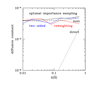
Figure 2: Efficiency versus importance function on a system with $N_{e}=N_{p}=16$ and $r_{s}=1.31$. In one system the protons are taken in a sc lattice and in the other they are displaced randomly, with an average displacement of $\Delta$. The diffusion constant is defined as $\Delta^{2}/T_{CPU}$ where $T_{CPU}$ is the computer time needed to calculate the energy difference to an accuracy of $1000~{}K$.

5 Choice of Trial Wave Function

An essential part of the CEIMC method is the choice of the trial wave function. Variational Monte Carlo (VMC) depends crucially on the trial wave function to find the minimum energy. The trial wave function is also important in DMC, to reduce the variance and the projection time, and for accurate nodal surfaces within the fixed-node method. CEIMC has special demands since optimization of a trial wave function must be done repeatedly, quickly and without direct user control.

A typical form of the variational wave function used in QMC is a Jastrow factor (two body correlations) multiplied by two Slater determinants of one body orbitals.

$$\psi_{T}=\exp\left[-\sum_{i<j}u(r_{ij})\right]{\mathrm{Det}}\left(S^{\uparrow}\right){\mathrm{Det}}\left(S^{\downarrow}\right)$$ (19)

The Slater determinant is taken from a mean field calculations such as Hartree–Fock or approximate density functional theory. The cusp condition can be used to well approximate this at short distances and RPA to determine the behavior at large distancesfoulkes .

In the molecular phase of hydrogen we estimated that using the orbitals determined from a separate DFT calculation would have been too slow. For the molecular phase we resort a simpler alternative namely we used gaussian single body orbitals, pinned in the center of the molecular bonds. Optimization of the gaussian, one for each of the molecules, took much of the computer time. See dewing00b ; dewing for a detailed discussion of those results.

For the metallic hydrogen phase, in a previous QMC investigation, Natolinatoli93 found that simple plane wave nodes are inaccurate by 0.05 eV/atom within the fixed-node approach at the transition to metallic hydrogen ($r_{s}=1.31$) necessitating the use of more accurate (LDA) nodes. However it is inconvenient and inefficient to solve the LDA equations for each new position of the ions in CEIMC. In addition, one has to modify the LDA orbitals to take into account the effect of explicit electron-electron correlation. The same problem of disordered ionic configurations arises from zero point motion of the protons in the solid state. In earlier work on molecular hydrogen, we were unable to use high quality LDA orbitals when the molecules were angularly disoriented natoli95 .

We have recently generalized the backflow and three–body wave function to a two component system of electrons and protons at high enough density so that the electrons are delocalized and all the hydrogen molecules are dissociated. For metallic hydrogen, as an element without a core, the formalism leading to the improved wave functions is simplest chep02 . These wave functions depend explicitly and continuously on the ionic variables and as a consequence do not have to be reoptimized for movements of the ions. These trial functions are a generalization of the backflow three–body wave functions used very successfully in highly correlated homogeneous quantum liquids: liquid ³He and electron gas. Backflow trial functions show much improvement over the pair product getting approximately 80% of the missing correlation and even more of the energy when done with the fixed-node method. Backflow wave functions utilize the power of the QMC sampling approach: one can calculate properties of such a wave function without changing the algorithm in an essential way, whileas in approaches based on explicit integration, one is limited in the form of the trial function by the ease performing the integration. We will discuss these backflow functions in more detail below.

6 Twist Average Boundary Conditions

Almost all QMC calculations in periodic boundary conditions have assumed that the phase of the wave function returns to the same value if a particle goes around the periodic boundaries and returns to its original position. However, with these boundary conditions, delocalized fermion systems converge slowly to the thermodynamic limit because of shell effects in the filling of single particle states. One can allow particles to pick up a phase when they wrap around the periodic boundaries,

$$\Psi(\vec{r}_{1}+L\hat{\vec{x}},\vec{r}_{2},\cdots)=\mathrm{e}^{i\theta_{x}}\Psi(\vec{r}_{1},\vec{r}_{2},\cdots).$$ (20)

The boundary condition $\theta=0$ is periodic boundary conditions (PBC), and the general condition with $\theta\neq 0$, twisted boundary conditions (TBC). The use of twisted boundary conditions is commonplace for the solution of the band structure problem for a periodic solid, particularly for metals. In order to calculate properties of an infinite periodic solid, properties must be averaged by integrating over the first Brillouin zone.

For a degenerate Fermi liquid, finite-size shell effects are much reduced if the twist angle is averaged over: twist averaged boundary conditions (TABC). This is particularly important in computing properties that are sensitive to the single particle energies such as the kinetic energy and the magnetic susceptibility. By reducing shell effects, much more accurate estimations of the thermodynamic limit for these properties can be obtained. What makes this even more important is that the most accurate quantum methods have computational demands which increase rapidly with the number of fermions. Examples of such methods are exact diagonalization (exponential increase in CPU time with N), variational Monte Carlo (VMC) with wave functions having backflow and three-body terms kwon2d ; kwon3d (increases as $N^{4}$), and transient-estimate and released-node Diffusion Monte Carlo methods cep84 (exponential increase with N). Methods which can extrapolate more rapidly to the thermodynamic limit are crucial in obtaining high accuracy.

Twist averaging is especially advantageous in combination with CEIMC (i.e. QMC) because the averaging does not necessarily slow down the evaluation of energy differences, except for the necessity of doing complex rather than real arithmetic. In a metallic system, such as hydrogen at even higher pressure when it becomes a simple metal, results in the thermodynamic limit require careful integration near the Fermi surface because the occupation of states becomes discontinuous. Within LDA this requires “k–point” integration, which slows down the calculation linearly in the number of k-points required. Within QMC such k-point integration takes the form of an average over the (phase) twist of the boundary condition and can be done in parallel with the average over electronic configurations without significantly adding to the computational effort. We typically spawn about 100 distinct QMC processes, run for a fixed time, and then average the resulting properties.

7 Fluid Molecular Hydrogen

We now describe our calculations on liquid molecular hydrogen. First of all, we examine the accuracy of several methods for computing total energy. We took several configurations from PIMC simulations at 5000 K at two densities ($r_{s}=1.86$ and $r_{s}=2.0$), and compared the electronic energy using VMC, DMC, DFT-LDA, and some empirical potentials. The DFT–LDA results were obtained from a plane wave code using an energy cutoff of 60 Rydbergs, and using the $\Gamma$ point approximation ogitsu00 . The empirical potentials we used are the Silvera–Goldman silvera78 and the Diep–Johnson diep00a ; diep00b . To these we added the energy from the Kolos kolos64 intramolecular potential to get the energy as a function of the bond length variations. The Silvera–Goldman potential was obtained by fitting to low temperature experimental data, with pressures up to 20 Kbar, and is isotropic. The Diep–Johnson potential is the most recent in a number of potentials for the isolated H₂–H₂ system. It was fit to the results of accurate quantum chemistry calculations for a number of H₂–H₂ configurations and included anisotropic effects in the potential.

The energies relative to an isolated H₂ molecule are shown in Figure 3. The first thing we notice is that the classical potentials are more accurate than VMC or DFT. The Silvera–Goldman does a good job of reproducing the DMC results. Some of the failures of the SG potential can be attributed to the lack of anisotropy. The isolated H₂–H₂ potential (Diep–Johnson) has much weaker interactions, compared with interactions in a denser system.

Figure 3: Electronic energy for several configurations computed by various methods. The energy is relative to an isolated H₂ molecule.

The PIMC method itself gives an average energy of about $0.07(3)$ Ha for both densities. Improvements in the fermion nodes and in other aspects of the PIMC calculation appear to lower the energy militzer00a ; militzer00b ; militzer-thesis00 , although the error bars are still quite large. The PIMC energy is in rough agreement with the DMC energy.

As mentioned above, we used the Silvera–Goldman potential for pre–rejection. As seen in the Figure 3, it resembles the DMC potential even though it lacks anisotropy. Each trial move consisted of moving multiple molecules (usually four). This increased efficiency by amortizing the cost of the QMC calculation. Each molecular move was decomposed into a translation of the center of mass, a rotation of the molecule, and a change in the bond length.

Shown in Tables 1–2 are CEIMC results at three state points, two of which can be compared with the gas gun data of Holmes et al. holmes95 . The pressure is given in table 1 with results from the gas gun experiments, the free energy model of Saumon and Chabrier saumon91 ; saumon92 ; saumon95 , from simulations using the Silvera–Goldman potential, and from our CEIMC simulations. These state points are in the fluid molecular H₂ phase. For the gas gun experiments, the uncertainties in the measured temperatures are around 100–200 K. The experimental uncertainties in the volume and pressure were not given, but previous work indicates that they are about 1–2% nellis83 .

We did CEIMC calculations using VMC or DMC for computing the underlying electronic energy, which are the first such QMC calculations in this range. The simulations at $r_{s}=2.1$ and $r_{s}=1.8$ were done with 32 molecules, and the simulations at $r_{s}=2.202$ were done with 16 molecules. We see that the pressures from VMC and DMC are very similar, and that for $r_{s}=2.1$ we get good agreement with experiment.

There is a larger discrepancy with experiment at $r_{s}=2.202$. The finite size effects are fairly large, especially with DMC. We also did simulations at $r_{s}=2.1$ with 16 molecules and obtained pressures of $0.264(3)$ Mbar for CEIMC–VMC and $0.129(4)$ Mbar for CEIMC–DMC. The Silvera–Goldman potential showed much smaller finite size effects than the CEIMC simulations, so we conclude that the electronic part of the simulation is largely responsible for the observed finite size effects.

The energies for all these systems are given in Table 2. The energy at $r_{s}=2.1$ with 16 molecules for CEIMC–VMC is $0.0711(4)$ Ha and for CEIMC–DMC is $0.0721(8)$ Ha. The proton–proton distribution functions comparing CEIMC–VMC and CEIMC–DMC are shown in Figure 4. The VMC and DMC distribution functions look similar, with the first large intramolecular peak around $r=1.4$ and the intermolecular peak around $r=4.5$.

Table 1: Pressure from simulations and shock wave experiments

rs	T(K)	Pressure (Mbar)
		Gasgun	S–C	S–G	CEIMC–VMC	CEIMC–DMC
2.100	4530	0.234	0.213	0.201	0.226(4)	0.225(3)
2.202	2820	0.120	0.125	0.116	0.105(6)	0.10(5)
1.800	3000	-	-	0.528	-	0.357(8)

Table 2: Energy from simulations and models, relative to the ground state of an isolated H₂ molecule. The H₂ column is a single thermally excited molecule plus the quantum vibrational KE.

rs	T(K)	Energy (Ha/molecule)
		H2	S–C	S–G	CEIMC–VMC	CEIM-C-DMC
2.100	4530	0.0493	0.0643	0.0689	0.0663(8)	0.0617(2)
2.202	2820	0.0290	0.0367	0.0408	0.0305(8)	0.0334(9)
1.800	3000	0.0311	-	0.0722	-	0.048(1)

(a)	(b)

Figure 4: Proton pair distribution, $g(r)$, for (a) $r_{s}=2.1$ and T=4530 K (b) $r_{s}=2.202$ and T=2820 K

The CEIMC–VMC simulations at $r_{s}=1.8$ and 3000 K never converged. Starting from a liquid state, the energy decreased during the entire simulation. Visualization of the configurations revealed that they were forming a plane. It is not clear whether it was trying to freeze, or forming structures similar to those found in DFT–LDA calculations with insufficient Brillouin zone samplinghohl93 ; kohanoff97 . (note that the molecular hydrogen calculations were done at the $\Gamma$ point.)The CEIMC–DMC simulations did not appear to have any difficulty, so it seems the VMC behavior was due to inadequacies of the wave function.

Hohl et al.hohl93 did DFT–LDA simulations at $r_{s}=1.78$ and T=3000 K, which is very close to our simulations at $r_{s}=1.8$. The resulting proton-proton distribution functions are compared in Figure 5. The CEIMC distribution has more molecules and they are more tightly bound. The discrepancy between CEIMC and LDA in the intramolecular portion of the curve has several possible causes. On the CEIMC side, it may be due to lack of convergence or to the molecular nature of the wave function, which does not allow dissociation. The shift of the molecular bond length peak can be accounted for because LDA is known to overestimate the bond length of a free hydrogen molecule hohl93 which would account for the shifted location of the bond length peak. The deficiencies of LDA may account for it preferring fewer and less tightly bound molecules.

Figure 5: The proton pair distribution function, $g(r)$, near $r_{s}=1.8$ and T=3000K.

8 The atomic-metallic phase

In this section, we describe preliminary results for metallic atomic hydrogen from a recent implementation of the method using an improved wave functions including threebody and backflow terms and taking advantage of averaging over the twist angle to minimize size effects.

8.1 Trial wave function and optimization

We have seen that an important part of the CPU time is needed in the optimization of the molecular trial wave functions which contain a number of variational parameters proportional to the number of molecules and which need to be optimized individually for each protonic steps. A major improvement in the efficiency of the method can be achieved by using more sophisticated wave functions, namely analytic functions in terms of the proton positions which move with the protons and which depend on few variational parameters (about 10, regardless of the number of particles). Moreover, one can explore the possibility of optimizing the variational parameters only once at the beginning of the calculation, either on ordered or disordered protonic configurations, and using the optimized wave function during the simulation. In this section, we consider hydrogen at densities at which molecules are dissociated ($r_{s}\leq 1.31$) and the system is metallic. We will therefore avoid the complications arising from the presence of bound states (either molecular or atomic). In this case one can show that improved wave functions with respect to the simple Slater-Jastrow form includes backflow and threebody terms between electrons and protons chep02 in a very similar fashion as the ones used by Kwon et al.kwon2d ; kwon3d for the electron gas. We assume a trial wave function of the form

$$\Psi_{T}(\vec{R})=det(e^{i{{\bf k}_{i}\cdot{\bf x}_{j}}})exp\left(-\sum_{i<j}^{N}\tilde{u}(r_{ij})-\frac{\lambda_{T}}{2}\sum_{l=1}^{N}{\bf G}(l)\cdot{\bf G}(l)\right)$$ (21)

where

$${\bf x}_{i}={\bf r}_{i}+\sum_{j\neq i}^{N}\eta(r_{ij})({\bf r}_{i}-{\bf r}_{j})$$ (22)

$${\bf G}(l)=\sum_{i\neq l}^{N}\xi(r_{li})({\bf r}_{l}-{\bf r}_{i})$$ (23)

$$\tilde{u}(r)=u(r)-\lambda_{T}\xi^{2}(r)r^{2}$$ (24)

with

$$\eta(r)=\lambda_{b}exp[-(r-r_{b})^{2}/w_{b}^{2}]$$ (25)

$$\xi(r)=exp[-(r-r_{T})^{2}/w_{T}^{2}]$$ (26)

and $u(r)$ is an optimized version of the RPA pseudopotential ca87 .

In what follows we only consider the effect of electron–proton backflow and electron–proton–proton three body terms, while the electronic part of the wave function is of the simple Slater–Jastrow form. To establish the goodness of this wave function for metallic hydrogen we perform VMC and DMC calculation for 16 protons on a bcc lattice at $r_{s}=1.31$. In table [3] we compare the energy and the variance of the local energy of this wave function with data obtained with the simple Slater-Jastrow wavefunction and with an improved wavefunction in which a determinant of single body orbital from a separate LDA calculation has been used natoli93 . From these results we infer that the nodes of the new wavefunction are as accurate as the LDA nodes.

Table 3: $r_{s}=1.31$. Energy and variance for 16 protons in the bcc lattice. SJ, SJ3B and LDA indicate optimized Slater–Jastrow, optimized Slater–Jastrow+three–body+backflow, and LDA nodes respectively. Energies per particle are in Rydbergs.

	$E_{VMC}$	$\sigma_{VMC}^{2}$	$E_{DMC}$
SJ	-0.4754(2)	0.0764(9)	-0.4857(1)
SJ3B	-0.4857(2)	0.0274(2)	-0.4900(1)
LDA	-0.4870(10)		-0.4890(5)

Having established that our wavefunction at $r_{s}=1.31$ is as good as the most accurate wavefunction used for metallic hydrogen so far, we continue our study at slightly higher density, namely $r_{s}=1$. It can be shown that the above form of the wavefunction is obtained using perturbation theory from the high density limit and we expect that its accuracy improves for decreasing $r_{s}$.

We first perform a number of optimizations of the trial wave function. Beside the RPA e–p Jastrow, we consider an extra 2 body (e–p) gaussian term with two variational parameters ($\lambda_{e}$ and $w_{e}$). In table 4 we report the values of the variational parameters obtained minimizing a linear combination of the local energy and its variance over a set of different protons and electrons configurations. Typically 1000 configurations have been used, by saving a configuration after 10 or 20 protonic steps during a previous run. We also studied the relative importance of the different terms in the trial wavefunction by performing calculations with partially improved wave functions. In Figure 6 we compare the pair correlation functions for the various calculations in table 4. No significant difference is observed in the electron–electron and in the proton–proton pair correlation functions among different forms of the trial function. We can see that the cooperative effects of the optimized Jastrow factor and the backflow term are responsible of an enhancing of electron-proton correlation as seen in the $g_{ep}(r)$. Inclusion of three–body terms lowers the energy but does not change the pair correlations.

Table 4: $r_{s}=1,T=5000\,K,N_{p}=N_{e}=16$. Optimized values of the variational parameters for the VMC trial function. The values are obtained minimizing local energy and variance for 1000 different equilibrium configurations.

	$\lambda_{b}$	$r_{b}$	$w_{b}$	$\lambda_{T}$	$r_{T}$	$w_{T}$	$\lambda_{e}$	$w_{e}$	E(a.u.)
SJ	–	–	–	—	–	–	–	–	-0.117(1)
SJE	—	—	—	–	–	–	0.06167	0.9497	-0.1180(4)
SJB	-0.60824	-1.3726	1.44822	–	–	–	–	–	-0.1207(4)
SJEB	-0.45828	-0.60202	0.91273	–	–	–	-0.0874	1.7002	-0.1227(5)
SJE3B	-0.4671	-0.6217	1.0193	-2.4676	-1.0917	3.0029	-0.0844	1.5130	-0.1238(2)

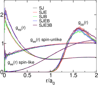
Figure 6: $r_{s}=1,T=5000\,K,N_{e}=N_{p}=16$ spin unpolarized. Pair correlations functions with various trial wave functions. The entries in the legend corresponds to the entries in table 4. The $g_{ep}(r)$ have been shifted downward by 0.5 for sake of clarity.

In principle, the optimization study could be repeated at each temperature needed for the CEIMC simulation. It is therefore of practical interest to investigate the transferability at finite temperature of wavefunctions optimized for the lattice configurations of protons.

An additional ingredient discussed above and crucial for a metallic system are finite size effects. It has been shown recently lzc01 that the very irregular behavior of the energy versus N observed in the presence of a Fermi surface can be reduced to the classical $1/N$ behaviour by averaging over the twist of the wavefunction. We have implemented the twist averaged boundary conditions in the calculation of the energy differences needed to make the protonic moves in the CEIMC. We average over 1000 different twist angles in the three dimensional interval $(-\pi,\pi)$ found to be sufficient in the electron gaslzc01 . The additional issue of whether optimization of the variational parameters need to be done with or without twist averaging was investigated. We compare in table 5 the results of single phase optimization and phase averaging optimizations for protons in the bcc lattice and at T=5000 K. The fourth row is the result of an optimization with twist averaging at T=0 K, while the fifth row is a run with the values of the variational parameters optimal for the $\Gamma$ point, always at T=0 K. We observe an excellent agreement of the energies and we conclude that we can safely optimize the wave function using the $\Gamma$ point and use the obtained variational parameters for all twist angles.

The sixth row in the table is the result of a simulation at T=5000 K using the values of the variational parameters optimal for T=0 K (bcc lattice). The energy should be compared with the result of the entry SJE3B in table 4. The difference in energy is within error bars and indicates that we can safely optimize the wave function on lattice configurations for use at finite temperature to avoid repeating the optimization at each temperature. In the last two rows of table 5 we report results of two runs at T=5000 K with twist averaging. In the first run the variational parameters optimized in the bcc configuration and with the $\Gamma$ point have been used. In the second one new values of the parameters, obtained by optimization over a set of configurations stored in the previous twist-averaged run, have been used. The excellent agreement on the energy (and on the variance of the local energy, not shown in the table) confirms that optimization of the variational parameters can be safely performed in the lattice configuration and with a single phase.

Table 5: $r_{s}=1,N_{p}=N_{e}=16$ spin unpolarized. Optimized values of the variational parameters for the VMC trial function. The values are obtained minimizing local energy and variance for 1000 different equilibrium configurations.

T(K)	#phases	$\lambda_{b}$	$r_{b}$	$w_{b}$	$\lambda_{3}$	$r_{3}$	$w_{3}$	$\lambda_{e}$	$w_{e}$	E(a.u.)
0	1	–	–	–	—	–	–	–	–	-0.1306(2)
0	1	-0.2574	-0.2172	0.7623	-2.3742	-1.8150	1.9694	-0.0496	1.7937	-0.1353(1)
0	1000	–	–	–	–	–	–	–	–	-0.1779(1)
0	1000	-0.2386	-0.1757	0.6613	-2.2609	-1.8326	3.3130	-0.0475	2.0337	-0.18254(3)
0	1000	-0.2574	-0.2172	0.7623	-2.3742	-1.8150	1.9694	-0.0496	1.7937	-0.18253(3)
5000	1	-0.2574	-0.2172	0.7623	-2.3742	-1.8150	1.9694	-0.0496	1.7937	-0.1237(2)
5000	1000	-0.2574	-0.2172	0.7623	-2.3742	-1.8150	1.9694	-0.0496	1.7937	-0.1708(3)
5000	1000	-0.4611	-0.7339	1.1287	-2.0402	-2.2098	3.0213	-0.0949	1.2389	-0.1709(3)

8.2 Comparison with PIMC

In order to establish the accuracy of the CEIMC method, we compare CEIMC and PIMC results at high temperatures and pressures. To eliminate the “fermion sign problem”, the R-PIMC technique for fermions assumes the nodal surfaces of a trial density matrix. In most of the applications, free particle nodal surfaces, either temperature dependent or in the ground state, have been usedhelium3-92 ; pcbm94 ; como95 . More recently, variational nodes which account for bound states have been implemented in the study of the plasma phase transition militzer00a ; militzer00b . However, the use of temperature dependent nodes, which break the imaginary time translational symmetry, is limited to quite high temperature, $T\geq 0.1T_{F}$ where $T_{F}(a.u.)=1.84158/r_{s}^{2}$ is the electronic Fermi temperature. Below this threshold, the Monte Carlo sampling becomes extremely inefficient and the method impractical. This pathology is not encountered when using ground state nodes, which preserve the original imaginary-time symmetry and are expected to become as accurate as the temperature dependent nodes at low enough temperature. At $r_{s}=1$ ($0.1T_{F}=0.18158a.u.\approx$ 57300 K), we perform calculation at T=10000 K and T=5000 K and we exploit the PIMC with free particle ground state nodes. In table 6 we compare energies and pressure from PIMC and CEIMC simulations. At T=10000 K, two different PIMC studies are reported, with $M=500$ and $M=1000$ time slices respectively, which correspond to $\tau=0.063(a.u.)^{-1}$ and $\tau=0.0315(a.u.)^{-1}$. The smaller value satisfy the empirical criteria for good convergence $\tau\leq 0.05/r_{s}^{2}(a.u.)^{-1}$ we have established in the plasma phase at higher temperature pcbm94 . At T=5000 K only $M=1000$ has been used and therefore the convergence with the number of time slices is limited.

We see small differences between PIMC and CEIMC. In particular, the electronic kinetic energy in PIMC is always slightly higher than in CEIMC. At the same time, CEIMC determined potential energy is lower than the PIMC value and this results in a significantly lower total energy of CEIMC compared to PIMC. The difference between PIMC and CEIMC seems to decrease with temperature. To judge the quality of these results, we should keep in mind advantages and limitations of each method. PIMC uses the “exact” bosonic action, the electrons are at finite temperature and excited states are taken into account, although in a approximate way because of the simplified nodal restriction: its approximation for the nodal surface is a Slater determinant of plane waves. CEIMC instead assumes a trial functions which, at the correlation (bosonic) level is certainly an approximation to the true bosonic action used in PIMC. Moreover, the electrons are in their ground state by construction. However, the trial wavefunction in CEIMC is better (for the ground state) than the one used in PIMC. Because of these differences we think that the comparison between the two methods shows agreement although a more detailed investigation is in order.

Table 6: $r_{s}=1,N_{p}=N_{e}=18$. Comparison between PIMC and CEIMC methods at T=10000 K and T=5000 K.

method	$T/10^{3}(K)$	M	$K_{e}/N_{e}$	$K_{t}/N$	$V_{N}/N$	$E/N$	$P$
PIMC	10	500	1.477(9)	0.763(5)	-0.7771(6)	-0.0141(6)	0.119(2)
PIMC	10	1000	1.48(1)	0.764(6)	-0.7820(8)	-0.0180(7)	0.119(2)
CEIMC	10	–	1.3767(4)	0.7121(2)	-0.7995(2)	-0.0874(4)	0.0994(1)
PIMC	5	1000	1.39(1)	0.707(5)	-0.791(1)	-0.084(6)	0.099(2)
CEIMC	5	–	1.317(1)	0.6703(3)	-0.7939(2)	-0.1236(2)	0.0870(8)

Comparison between PIMC and CEIMC for the pair correlation functions at T=10000 K and T=5000 K is given in Figures 7 and 8 respectively. In Figure 7 we first note a good agreement between the two PIMC calculations which show that pair correlation functions are much less sensible to finite imaginary time step errors. In general for all correlation functions except the electron-proton ones, the agreement between PIMC and CEIMC is excellent.

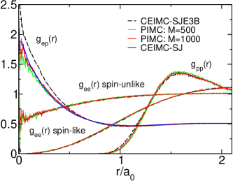
Figure 7: Pair correlation functions at T=10000 K. Comparison between PIMC and CEIMC. $g_{ep}(r)$ have been shifted by $-0.5$ for sake of clarity.

At T=10000 K the electron–proton pair correlation function from PIMC is in very good agreement with the result of the CEIMC method where a simple Slater–Jastrow trial wave function is used. Improving the trial wave function as discussed in the previous subsection worsen the agreement. The opposite behavior is observed at T=5000 K where the better agreement between PIMC and CEIMC is observed with the improved wave function (SJE3B in the Figure). We interpret this behaviour as follows: at lower temperature the improved trial wave function (21) provides the “correct” electron–proton correlation (through the combined effect of the optimized Jastrow and the electron–proton backflow, see the discussion relative to Figure 6 in the previous subsection). At this temperature the electronic thermal effects on the electron–proton correlation are quite small and the electronic ground state as provided by CEIMC is quite accurate. Instead at higher temperatures electron–proton scattering is influenced by excited electronic states which are not considered in the CEIMC method. As a result the electron–proton pair correlation function shows a weaker correlation near the origin and it is in better agreement with the CEIMC result with the Slater–Jastrow trial function rather than with the CEIMC result for the improved trial function.

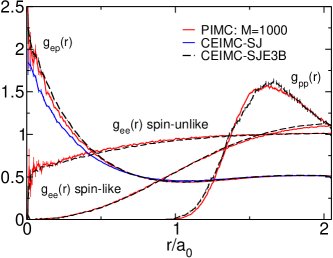
Figure 8: Pair correlation functions at T=5000 K. Comparison between PIMC and CEIMC. $g_{ep}(r)$ have been shifted by $-0.5$ for sake of clarity.

8.3 Hydrogen equation of state and solid–liquid phase transition of the protons

We present in this subsection, results for the equation of state (EOS) of hydrogen in the metallic phase including the solid–liquid transition of protons. These results are preliminary in various respects. Firstly, the electrons are treated at the variational level and no use of Projection/Diffusion Monte Carlo was attempted. Secondly, the protons are considered as classical point particles although it is well known that zero point motion at such high pressure can be significant (at least around the phase transition). Finally, we have data at a single density ($r_{s}=1$) and for a single system size, namely $N_{e}=N_{p}=32$ (compatible with the fcc lattice) and we cannot address, at this stage, the issue of the relative stability of different crystal structures. Nonetheless, we believe these results are interesting because they show the applicability and provide a benchmark of the method.

In table 7, we report various details of the simulations such as the maximum amplitude of the protonic step in units of the Bohr radius $\Delta_{p}$, the total number of electronic steps per protonic step $M_{el}$, the relative noise level for the penalty method $(\beta\sigma)^{2}$, the acceptance for the protonic move and the noise rejection ratio $\eta$ dewing . A measure of the computational efficiency can be defined as the proton diffusion in configurational space with respect to the CPU time $D_{p}=(\sum_{p}[\Delta R_{p}]^{2})/T_{CPU}$. In the table we report the values obtained in our simulations in units of $a_{0}^{2}/sec$. In addition, the CPU time per protonic step, the number of processors and the machine used are reported.

Note that $M_{el}=15000$ is the minimum number of electronic steps needed to average over 1000 different twist angles. Except at the lowest temperatures ($T\leq$500 K) such large number of electronic steps would not be necessary in order to reduce the noise level. Further improvements in efficiency could be gained by reducing the number of electronic steps or the number of angles averaged over for $T>500\,K$.

Table 7: Simulation details: $r_{s}=1,N_{p}=N_{e}=32$. $\Delta_{p}$ is the maximum amplitude of the protonic step in units of the Bohr radius, $M_{el}$ is the total number of electronic steps per protonic step, $(\beta\sigma)^{2}$ is the relative noise level entering in the penalty method, $P_{acc}$ is the average acceptance of the protonic moves, $\eta$ is the noise rejection ratio defined earlier, $D_{p}$ is the diffusion constant in protonic configurational space with respect to CPU time.

$T(K)$	$\Delta_{p}$	$M_{el}$	$(\beta\sigma)^{2}$	$P_{acc}$	$\eta$	$D_{p}\times 10^{4}$	time/step(sec)	#proc	machine
5000	0.03	15000	0.037(4)	0.80	0.0084	1.9(2)	5.96	32	beowulf
4000	0.03	15000	0.092(8)	0.77	0.013	3.8(3)	5.93	32	beowulf
3000	0.025	15000	0.10(2)	0.76	0.012	3.2(3)	10.3	16	origin3800
2000	0.03	15000	0.29(5)	0.68	0.033	2.6(3)	10.3	16	origin3800
1000	0.02	15000	0.30(3)	0.64	0.06	3.6(3)	10.3	16	origin3800
700	0.02	15000	0.418(4)	0.55	0.10	3.6(3)	9.90	16	origin3800
500	0.02	15000	0.747(5)	0.43	0.16	0.47(8)	8.93	32	platinum
300	0.015	18000	0.855(9)	0.39	0.21	0.18(1)	7.02	32	platinum

In table 8 we report thermodynamic quantities for the system at various temperatures in the range $T\in$[300 K,5000 K]. The corresponding electron–protons and protons–protons pair correlation functions are given in Figures 9 and 10 respectively. At each temperature, equilibrium runs of at least 20000 protonic steps have been performed. Statistics are collected every 20–50 steps. Besides energies and pressure we compute the Lindemann ratio $\gamma$ for the fcc structure. In the upper part of the table, i.e. at higher temperature, we report in the last column the status of the system. At T=1500 K the system initially in the fcc configuration is found to melt after few thousands steps. Conversely at T=500 K we started the simulation in a disordered state and the system spontaneously ordered into the fcc structure. At T=1000 K instead, a system starting in a lattice configuration remains solid and a system starting from a liquid configuration remains liquid within the length of the runs. The Lindemann criterion for classical melting locates the transition at the temperature at which $\gamma\simeq 0.15$. From the result in the table the fcc–liquid transition temperature should be located between 1000 K and 1500 K. Previous investigation of such a transition has been performed by Car–Parrinello Molecular Dynamics kh96 . This study suggests that at $r_{s}=1$ the structure of the system at $T=0K$ is hcp but for $T>$100 K the bcc structure is more favorable (as in this work, protons were considered as classical particles). The melting temperature of the bcc lattice has been estimated by the Lindemann criterion around 350 K, significantly lower than the present estimate. We are presently investigating the system of 54 protons in order to study the stability of the bcc structure and the melting transition temperature.

Table 8: $r_{s}=1,N_{p}=N_{e}=32$, spin unpolarized

$T(K)$	$K_{tot}$	$V_{c}$	$E_{tot}$	$\sigma_{E}^{2}$	$P(Mbars)$	$\gamma$
5000	0.6241(2)	-0.7820(1)	-0.1579(2)	0.056(2)	21.72(2)	liquid
4000	0.0620(2)	-0.7821(2)	-0.1619(1)	0.055(3)	21.35(1)	liquid
3000	0.0616(1)	-0.7817(1)	-0.1662(2)	0.051(7)	20.93(1)	liquid
2000	0.06122(6)	-0.7842(1)	-0.1702(1)	0.050(2)	20.588(6)	liquid
1500	0.61113(7)	-0.7848(1)	-0.1737(1)	0.046(1)	20.374(6)	melted
1000	0.60847(6)	-0.78372(8)	-0.17525(4)	0.0446(5)	20.181(3)	liquid
1000	0.60894(5)	-0.78549(9)	-0.17655(7)	0.0416(5)	20.143(3)	0.137(4)
700	0.60787(3)	-0.78614(5)	-0.17817(8)	0.0402(6)	20.017(6)	0.109(2)
500	0.60811(3)	-0.78718(3)	-0.17913(5)	0.048(4)	19.985(3)	0.085(3)
300	0.60680(4)	-0.78686(2)	-0.18017(2)	0.042(3)	19.874(3)	0.083(1)

Figure 9: $r_{s}=1,N_{e}=N_{p}=32$ spin unpolarized. Temperature dependence of the electron–proton pair correlation functions. The y scale is logarithmic.

Figure 10: $r_{s}=1,N_{e}=N_{p}=32$ spin unpolarized. Temperature dependence of the proton–proton pair correlation functions. The difference between the crystal and the liquid is clearly seen.

9 Conclusions and Outlook

In this article we have discussed the CEIMC method, along with a number of supporting developments to make it computationally efficient. Using the penalty method, we have shown how it is possible to formulate a classical Monte Carlo, with the energy difference having statistical noise, without affecting the asymptotic distribution of the protons. We have made significant progress on several related issues: the computation of energy differences, the development of wavefunctions that do not require optimization of variational parameters and use of twist averaged boundary conditions. We have applied the method to an important many-body system, molecular and metallic hydrogen at high pressure. We have shown that the method is feasible on current multi-processor computers.

One of the advantages of QMC over DFT, in addition to higher accuracy, is the different way basis sets enter. Single particle methods usually work in a “wave basis”, where the wave function is expanded in plane waves or Gaussian orbitals. In contrast QMC uses a particle basis. A smooth basis (the trial wave function) is indeed used within VMC, however, cusps and other features are easily added without slowing down the computation. For this reason, the bare Coulomb interaction can be easily treated, while in LDA, typically a smooth pseudopotential is needed, even for hydrogen, to avoid an excessive number of basis functions.

As shown in the example of twist-averaged boundary conditions, the CEIMC method has further advantages when additional averages are to be performed. In the present calculation, we assumed classical protons for simplicity. Of course, quantum effects of the protons are important and have been included in previous QMC and LDA calculations. But it is not hard to see that it is possible to do path integrals of the nuclei within the penalty method for very little increased cost over classical nuclei. A path integral simulation creates a path of $M$ slices, with each slice at an effective temperature of $MT$. We then need to perform $M$ separate electronic simulations, one for each slice. However, the penalty method requires the error level to be approximately $k_{B}T$. Then the required error level at each slice is $Mk_{B}T$, so each of the $M$ separate QMC simulations need not be as accurate. In contrast, for PI-LDA calculations, $M$ time slices will take $M$ times as long.

Our impression is that the CEIMC method on this application of high pressure hydrogen has the same order of computational demands as Car-Parrinello plane-wave methods: our results suggest that the CEIMC method may turn out to be both more accurate and faster. The processing power of current multi-processors is enough that significant applications are being pursued, giving much more accurate results for systems of hydrogen and helium including all effects of electron correlation and quantum zero point motion. In general, we expect the CEIMC method to be most useful when there are additional averages to be performed perhaps due to disorder or quantum effects. On the other hand DFT methods are more efficient for optimizing molecular geometries where the existing functional are known to be locally accurate or for dynamical studies outside the scope of CEIMC.

Tests for non-hydrogenic systems are needed to find the performance of the algorithms on a broader spectrum of applications. The use of pseudopotentials within QMC to treat atoms with inner core is well tested. What is not clear is how much time will be needed to generate trial functions, and to reduce the noise level to acceptable limits. Also interesting is to develop a dynamical version of CEIMC, i.e. CEIMD. Many of the techniques discussed here such as twist averaging, advanced trial functions and energy difference methods are immediately applicable. However, while it is possible within MC to allow quantum noise, it is clear that the noise level on the forces must be much smaller, since otherwise the generated trajectories will be quite different. The effect of the quantum noise, in adding a fictitious heat bath to the classical system, may negate important aspects of the rigorous approach we have followed. One possible approach is to locally fit the potential surface generated within QMC to a smooth function, thereby reducing the noise level. Clearly, further work is needed to allow this next step in the development of microscopic simulation algorithms.

References

- (1) N. Metropolis, A. W. Rosenbluth, M. N. Rosenbluth, A. H. Teller, and E. Teller: J. Chem. Phys. 21, 1087 (1953)
- (2) R. G. Parr and W. Yang. Density Functional Theory of Atoms and Molecules, Oxford, 1989.
- (3) R. Car and M. Parrinello: Phys. Rev. Lett. 55, 2471 (1985)
- (4) M. C. Payne, M. P. Teter, D. C. Allan, T. A. Arias, and J. D. Joannopoulos: Rev. Mod. Phys 64, 1045 (1992)
- (5) D. Marx and M. Parrinello: J. Chem. Phys. 104, 4077 (1996)
- (6) M. Sprik: J. Phys.: Condens. Matter 12, A161 (2000)
- (7) M. E. Tuckerman and G. J. Martyna: J. Phys. Chem. B 104, 159 (2000)
- (8) W. M. C. Foulkes et al.: Rev. Mod. Phys. 73, 33 (2001)
- (9) B. L. Hammond, Jr. W. A. Lester, and P. J. Reynolds. Monte Carlo Methods in Ab Initio Quantum Chemistry, World scientific lecture and course notes in chemistry, (World Scientific, Singapore, 1994)
- (10) J. B. Anderson:‘Exact quantum chemistry by Monte Carlo methods’ In Quantum Mechanical Electronic Structure Calculations with Chemical Accuracy, ed. S. R. Langhoff, (Kluwer Academic, 1995)
- (11) D. M. Ceperley and L. Mitas:‘Quantum Monte Carlo methods in chemistry’. In Advances in Chemical Physics ed. by I. Prigogine and S. A. Rice, (Wiley and Sons, 1996)
- (12) J. C. Grossman, L. Mitas, and K. Raghavachari: Phys. Rev. Lett. 75, 3870 (1995)
- (13) M. Dewing: Monte Carlo Methods: Application to hydrogen gas and hard spheres. PhD thesis, University of Illinois at Urbana-Champaign (2000). Available as arXiv:physics/0012030.
- (14) W. B. Hubbard and D. J. Stevenson: ‘Interior structure’. In Saturn, ed. by T. Gehrels and M. S. Matthews (University of Arizona Press, 1984)
- (15) D. J. Stevenson:‘The role of high pressure experiment and theory in our understanding of gaseous and icy planets’. In Shock waves in condensed matter, ed. by S. C. Schmidt and N. C. Holmes (Elsevier, 1988)
- (16) B. Militzer and E. L. Pollock: Phys. Rev. E 61, 3470 (2000)
- (17) D. M. Ceperley and B. J. Alder: Phys. Rev. B 36, 2092 (1987)
- (18) V. Natoli, R. M. Martin, and D. M. Ceperley: Phys. Rev. Lett. 70, 1952 (1993)
- (19) V. Natoli, R. M. Martin, and D. M. Ceperley: Phys. Rev. Lett. 74, 1601 (1995)
- (20) M. Dewing and D. M. Ceperley: ‘Methods for Coupled Electronic-Ionic Monte Carlo’. In: Recent Advances in Quantum Monte Carlo Methods, II, ed. by S. Rothstein (World Scientific, Singapore), submitted Jan 2001.
- (21) P. J. Reynolds, D. M. Ceperley, B. J. Alder, and W. A. Lester: J. Chem. Phys. 77, 5593 (1982)
- (22) D. M. Ceperley and M. Dewing: J. Chem. Phys. 110, 9812 (1999)
- (23) D. M. Ceperley: Rev. Mod. Phys. 67, 279 (1995)
- (24) D. M. Ceperley, M. Holzmann, K. Esler and C. Pierleoni: Backflow Correlations for Liquid Metallic Hydrogen, to appear.
- (25) Y. Kwon, D.M. Ceperley and R. M. Martin: Phys. Rev. B 48, 12037 (1993)
- (26) Y. Kwon, D.M. Ceperley and R. M. Martin: Phys. Rev. B 58, 6800 (1998)
- (27) D. M. Ceperley and B. J. Alder: J. Chem. Phys. 81, 5833 (1984)
- (28) T. Ogitsu: ‘MP-DFT (multiple parallel density funtional theory) code, (2000) http://www.ncsa.uiuc.edu/Apps/CMP/togitsu/MPdft.html.
- (29) I. F. Silvera and V. V. Goldman: J. Chem. Phys. 69, 4209 (1978)
- (30) P. Diep and J. K. Johnson: J. Chem. Phys. 112, 4465 (2000)
- (31) P. Diep and J. K. Johnson: J. Chem. Phys. 113, 3480 (2000)
- (32) W. Kolos and L. Wolniewicz: J. Chem. Phys. 41, 1964.
- (33) B. Militzer and D. M. Ceperley: Phys. Rev. Lett. 85, 1890 (2000)
- (34) B. Militzer. Path Integral Monte Carlo Simulations of Hot Dense Hydrogen. PhD thesis, University of Illinois at Urbana-Champaign, 2000.
- (35) N. C. Holmes, M. Ross, and W. J. Nellis: Phys. Rev. B 52, 15835 (1995)
- (36) D. Saumon and G. Chabrier: Phys. Rev. A 44, 5122 (1991)
- (37) D. Saumon and G. Chabrier: Phys. Rev. A 46, 2084 (1992)
- (38) D. Saumon, G. Chabrier, and H. M. Van Horn: Astrophys. J. Sup. 99, 713 (1995)
- (39) W. J. Nellis, A. C. Mitchell, M. van Theil, G. J. Devine, R. J Trainor, and N. Brown: J. Chem. Phys. 79, 1480 (1983)
- (40) D. Hohl, V. Natoli, D. M. Ceperley, and R. M. Martin: Phys. Rev. Lett. 71, 541 (1993)
- (41) J. Kohanoff, S. Scandolo, G. L. Chiarotti, and E. Tosatti: Phys. Rev. Lett. 78, 2783 (1997)
- (42) C. Lin, F. H. Zong and D. M. Ceperley: Phys. Rev. E 64, 016702 (2001)
- (43) D. M. Ceperley; Phys. Rev. Lett. 69, 331 (1992)
- (44) C. Pierleoni, B. Bernu, D. M. Ceperley and W. R. Magro: Phys. Rev. Lett. 73, 2145 (1994); W. R. Magro, D. M. Ceperley, C. Pierleoni, and B. Bernu: Phys. Rev. Lett. 76, 1240 (1996)
- (45) D. M. Ceperley: ‘Path integral Monte Carlo methods for fermions’. In Monte Carlo and Molecular Dynamics of Condensed Matter Systems, ed. by K. Binder and G. Ciccotti (Editrice Compositori, Bologna, Italy, 1996)
- (46) J. Kohanoff and J. P. Hansen: Phys. Rev. E 54, 768 (1996)