Reaction Pathways Based on the Gradient of the Mean First-Passage Time

Abstract

Finding representative reaction pathways is necessary for understanding mechanisms of molecular processes, but is considered to be extremely challenging. We propose a new method to construct reaction paths based on mean first-passage times. This approach incorporates information of all possible reaction events as well as the effect of temperature. The method is applied to exemplary reactions in a continuous and in a discrete setting. The suggested approach holds great promise for large reaction networks that are completely characterized by the method through a pathway graph.

Introduction.

In many physical, chemical, or biological reactions, initial (reactant) and final (product) states are known but reaction pathways are not. Examples range in complexity from single-particle Brownian motion to conformational changes of proteins, such as protein folding Pande et al. (1998); Eastman et al. (2001). Finding reaction pathways is one of the most fundamental challenges in chemistry and molecular biologyElber (1996); Straub (2001). It is important for understanding reaction mechanisms and for the calculation of reaction rates Hänggi et al. (1990).

In most cases of interest, reactions take place at finite temperature and therefore are stochastic: every reaction event follows a different path and takes a different amount of time. Among all possible paths from reactant to product, one seeks the path that best characterizes the reaction not (a). The selection criteria are twofold. First, one seeks minimal paths, free of unnecessary fluctuations. Second, and more important, one seeks paths that are representative of all reaction events so that individual reaction events can be considered to be following noisy paths around them. It is, however, challenging to formulate these criteria rigorously.

The most widely used formulation of reaction path is probably the steepest-descent path, which is constructed by identifying saddle points of the potential energy surface and then following the steepest descent from the saddle points such that energy barriers along the path are minimized Elber (1996). The steepest-descent path, however, does not involve temperature. Since reactions are driven by thermal fluctuations, reaction paths should depend on temperature. For example, if there is a direct path with high energy barriers and a roundabout path with low energy barriers, at a temperature higher than the barriers reaction will occur most likely along the direct path rather than the roundabout path while the steepest-descent path will be the roundabout path regardless of temperature.

Understanding this drawback of the steepest-descent path has led to alternative formulations of reaction path. One approach is to select the path of maximum flux Berkowitz et al. (1983); Huo and Straub (1997). Another formulation focuses on most probable paths Pratt (1986); Elber and Shalloway (2000). In this approach, an ensemble of reaction events of a fixed time interval is considered. A probability is then assigned to each event, and the path followed by the most probable event is taken as the reaction path not (b).

The above methods succeeded to a certain extent in elucidating reaction mechanisms, but they do not fully satisfy the criterion of representativity. The method of most probable path comes closest to satisfying the criterion, but it is not clear how to choose the time interval beforehand and whether an ensemble of reaction events of a single time interval suffices to represent the reaction.

In this paper we present a new formulation of reaction path. While previous approaches attempted to quantify paths, we use the concept of reaction coordinate which quantifies states. Reaction coordinate is a function that describes where in the progress of reaction a state is located. The most natural measure of the progress of reaction is provided by the mean first-passage time (MFPT), namely the average amount of time that the system starting from the state takes to reach the given product. The MFPT depends on the energy landscape, the temperature, as well as the boundary conditions, and most important, it is an average over all reaction events. Surprisingly, to our knowledge, the MFPT has never been used as a reaction coordinate before. Once the MFPT is determined, one can choose as reaction paths the paths along which the MFPT decreases most rapidly, which complies with the criterion of minimal path.

Theory.

A practical scheme of determining reaction coordinates and reaction paths based on MFPTs can indeed be stated, as described below and illustrated in Fig. 1.

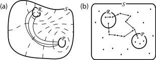
Figure 1: Schematic pictures of reaction paths. $\mathcal{S}$ is the set of all accessible states, $\mathcal{R}$ the reactant, and $\mathcal{P}$ the product. (a) A continuous system. Dashed lines are contours of the reaction coordinate (the MFPT to the product $\mathcal{P}$). In a Cartesian coordinate system, they are orthogonal to the reaction paths. (b) A discrete system. Dots are the accessible states.

Consider a system undergoing a stochastic reaction and let $\mathcal{S}$ be the set of all states that the system can access. If $\mathcal{S}$ is continuous the reaction can be described by a Fokker-Planck-type equation, and if $\mathcal{S}$ is discrete it can be described by a master equation Gardiner (1985). The reactant and the product are specified by disjoint subsets, $\mathcal{R}$ and $\mathcal{P}$ respectively, of $\mathcal{S}$. The reaction can be considered a first-passage process Redner (2001) because a reaction event ends as soon as the system reaches any state in $\mathcal{P}$. The MFPT $\tau(\mathbf{x})$ from state $\mathbf{x}$ to the product $\mathcal{P}$ is then calculated for all states $\mathbf{x}$ in $\mathcal{S}$ (this involves solving an inhomogeneous partial differential equation when $\mathcal{S}$ is continuous and inverting a transition matrix when discrete MFP ; Bauer et al. (1988), as demonstrated later) and is used as a reaction coordinate. The location of the reactant set $\mathcal{R}$ does not affect the calculation of the reaction coordinate $\tau(\mathbf{x})$; it is involved only in determining reaction paths.

The scheme of constructing reaction paths from MFPTs depends on the character of the set $\mathcal{S}$. When $\mathcal{S}$ is continuous and described by a Cartesian coordinate system, reaction paths are constructed following the direction of $-\nabla\tau$, along which $\tau$ decreases most rapidly. Thus, a reaction path $\mathbf{x}(l)$, parameterized through an arc length $l$, satisfies

$${dx_{i}\over dl}=v_{i}\Big{(}\sum\nolimits_{j}v_{j}v_{j}\Big{)}^{-1/2}\;,\quad v_{i}=-{\partial\tau\over\partial x_{i}}\;.$$ (1)

Often, reactions are better described with non-Cartesian coordinates such as angles. In such cases reaction paths can be determined via a transformation to a Cartesian coordinate system, and the resulting equation of reaction path is

$${dx_{i}\over dl}=v_{i}\Big{(}\sum\nolimits_{j}v_{j}v_{j}\Big{)}^{-1/2}\;,\quad v_{i}=-\sum\nolimits_{j}g^{-1}_{ij}{\partial\tau\over\partial x_{j}}\;.$$ (2)

Here $g^{-1}_{ij}$ is the inverse matrix of the metric tensor $g_{ij}$ and $l$ is now the arc length with respect to the non-Cartesian coordinate system ($dl^{2}\!=\!\sum_{i}dx_{i}dx_{i}$).

When $\mathcal{S}$ is discrete and the reaction is governed by a master equation with transition rates $k_{yx}$ (from state $x$ to state $y$), the MFPT $\tau_{x}$ from state $x$ to the product $\mathcal{P}$ is again employed as a reaction coordinate. But in order to determine reaction paths an analogue of metric is required, as reaction paths for continuous systems are determined via gradients which involve metric. The most obvious choice for an analogue of metric is the transition rates $k_{yx}$ themselves, and we suggest the scheme that a reaction path going through state $x$ chooses the next state $y$ such that $k_{yx}(\tau_{x}\!-\!\tau_{y})$ is maximized. For the transition step from $x$ to $y$, the transition time $1/k_{yx}$ may be interpreted as a cost, and the decrease $\tau_{x}\!-\!\tau_{y}$ in the MFPT as a gain. The scheme then amounts to maximizing the ratio between these two times, namely the gain-cost ratio, for each step.

According to the above scheme, a reaction path is constructed starting from each state in the reactant set $\mathcal{R}$. In general, multiple reaction paths are obtained unless the reactant set is narrowed down to a single state. Some reaction paths may overlap if they go through a common state.

Examples.

To demonstrate the above scheme and its outcomes, we consider first a single-particle Brownian motion on a two-dimensional potential surface described with a Cartesian coordinate system ($x_{1},x_{2}$). We take the three-hole potential

$$U(x_{1},x_{2}) = -3e^{-x_{1}^{2}-(x_{2}-5/3)^{2}}+3e^{-x_{1}^{2}-(x_{2}-1/3)^{2}}$$ (3)

$$-5e^{-(x_{1}-1)^{2}-x_{2}^{2}}-5e^{-(x_{1}+1)^{2}-x_{2}^{2}}$$

which was also studied by others regarding the temperature dependence of reaction paths Huo and Straub (1997); Elber and Shalloway (2000).

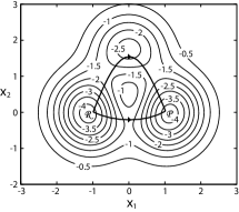
Figure 2: A contour plot of the three-hole potential, with two candidates for reaction path.

The potential features two deep holes and one shallow hole (Fig. 2). The two deep holes are considered as the reactant and the product. Roughly two possible pathways can be seen; the upper path is longer than the lower one but has lower energy barriers. It is therefore expected that the upper path will be taken at low temperature and that the lower path will be taken at high temperature.

The Brownian motion can be described in terms of the probability distribution $p(\mathbf{x},t)$ and the probability current $\mathbf{J}(\mathbf{x},t)$. In the strong friction regime, they satisfy the Smoluchowski equation Gardiner (1985)

$${\partial\over\partial t}p(\mathbf{x},t)=-\nabla\cdot\mathbf{J}(\mathbf{x},t)$$

$$\mathbf{J}(\mathbf{x},t)=-(\beta\gamma)^{-1}e^{-\beta U(\mathbf{x})}\nabla[e^{\beta U(\mathbf{x})}p(\mathbf{x},t)]\;,$$ (4)

where $\gamma$ is the friction coefficient. The MFPT $\tau(\mathbf{x})$ is then obtained by solving the inhomogeneous partial differential equation

$$\nabla\cdot[e^{-\beta U(\mathbf{x})}\nabla\tau(\mathbf{x})]=-\beta\gamma e^{-\beta U(\mathbf{x})}\;$$ (5)

with appropriate boundary conditions MFP . We take the region $(-4\!\leq\!x_{1}\!\leq\!4,-3\!\leq\!x_{2}\!\leq\!4)$ as the whole set $\mathcal{S}$, and assume that its boundary is reflecting, namely the probability current $\mathbf{J}$ is tangential to the boundary. For the reactant $\mathcal{R}$ we take the single point $(-1,0)$, and for the product $\mathcal{P}$ we take the circular region of radius 0.1 centered at $(1,0)$. Because a reaction event ends when the particle reaches the product region $\mathcal{P}$, the boundary of $\mathcal{P}$ is absorbing, with the probability distribution $p$ vanishing at the boundary. Boundary conditions for $p$ and $\mathbf{J}$ lead to corresponding boundary conditions for $\tau$: $\tau$ vanishes at absorbing boundaries and $\nabla\tau$ is tangential to reflecting boundaries MFP .

The solutions of Eq. (5), numerically obtained with MATLAB Mat , for two different temperatures are shown in Fig. 3.

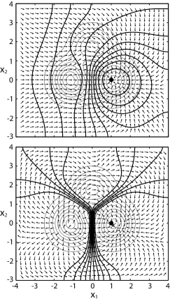
Figure 3: Reaction paths of the Brownian motion on the three-hole potential. Top, $\beta\!=\!1$; bottom, $\beta\!=\!8$. The directions of $-\nabla\tau$ at selected grid points are plotted as arrows. Contours of the reaction coordinate $\tau$ (thick lines) and the potential (thin lines) are shown. The product region is indicated by the filled circle.

The differences between the two temperatures are dramatic. At the high temperature ($\beta\!=\!1$) the arrows denoting the directions of $-\nabla\tau$ flow more or less directly towards the product. At the low temperature ($\beta\!=\!8$), on the other hand, the flow is significantly distorted so that energy barriers are avoided, with a singular point produced around $(-1.5,-0.5)$. Also, the reaction coordinate $\tau$ drops rapidly when barriers are crossed, as indicated by the contours of $\tau$ packed around saddle points.

Fig. 4 shows the reaction paths found at various temperatures.

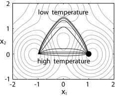
Figure 4: Temperature dependence of reaction paths of the Brownian motion on the three-hole potential. Shown are eight reaction paths for eight different temperatures, from bottom to top, $\beta\!=\!1,2,3,4,5,6,7,8$. The reactant is the point $(-1,0)$, and the product is the region indicated by the filled circle.

As was expected, lower paths are taken at high temperature and upper paths are taken at low temperature. At intermediate temperature, such as $\beta\!=\!4$, reaction paths lie in between, indicating that the upper and lower paths are equally favorable.

In order to demonstrate the scheme for reaction paths of discrete systems, we consider light-harvesting complexes Blankenship (2002); LH ; Damjanović et al. (2002), choosing photosystem I of cyanobacterium Synechococcus elongatus as an example. Photosystem I is a protein-pigment complex, embedded in the cell membrane, that contains 96 chlorophylls. The aggregate of these chlorophylls is responsible for the first step in photosynthesis, namely absorption of light and subsequent migration of the resulting electronic excitation towards the special pair of chlorophylls, called P700 and located at the geometrical center of the aggregate, where the next step in photosynthesis, the charge separation, occurs. This excitation migration can be considered a reaction. Assuming that no more than a single chlorophyll is simultaneously excited in the system, the states are specified by the excited chlorophylls. The reactant is specified by the chlorophyll that initially absorbed a photon; the product is specified the P700 pair of chlorophylls. Reaction paths of this system provide representative and minimal pathways of the excitation migration from the initially excited chlorophyll to the P700 pair.

Since we are interested in first passage of excitation to P700, it is convenient to consider a subsystem of 94 chlorophylls, excluding the P700 pair of chlorophylls. The migration of excitation in this subsystem can be described by the master equation

$${d\over dt}p_{x}(t)=\sum\nolimits_{y}K_{xy}\,p_{y}(t)\;,$$ (6)

where $p_{x}(t)$ is the probability that the excitation resides at chlorophyll $x$ at time $t$ and $K_{xy}$ is a $94\!\times\!94$ transition matrix Ritz et al. (2001); Park et al. . We build the transition matrix $K_{xy}$ by using the inter-chlorophyll excitation transfer rates that were calculated in Ref. Şener et al. (2002) based on the theory developed in Damjanović et al. (1999) and the recently obtained structure of photosystem I Jordan et al. (2001). The MFPT $\tau_{x}$ from chlorophyll $x$ to the P700 pair is then Park et al.

$$\tau_{x}=-\sum\nolimits_{y}\phi_{y}K^{-1}_{yx}\Big{/}\phi_{x}\;,\quad\phi_{x}=-\sum\nolimits_{y}\xi_{y}K^{-1}_{yx}\;.$$ (7)

Here $K^{-1}_{xy}$ is the inverse matrix of $K_{xy}$ and $\xi_{x}$ is the excitation transfer rate from chlorophyll $x$ to P700. The reaction paths constructed from the MFPT are shown in Fig. 5.

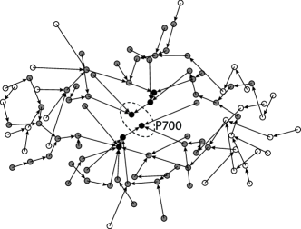
Figure 5: Reaction paths of the excitation migration in photosystem I. The positions of the chlorophylls, projected onto the membrane plane, are denoted by circles colored according to the MFPT: black, short MFPT; gray, intermediate MFPT; white, long MFPT.

A detailed discussion of this system is reported in Park et al. .

Conclusion.

We have presented a new method to construct reaction paths based on the MFPT gradient that incorporates all reaction events, and illustrated how it captures important aspects of reactions, most notably temperature effects. Unlike previous attempts, the present method provides paths starting from all states of the system. We believe that the MFPT is the most natural choice for reaction coordinate, and expect that our approach will be used in many future studies of reactions. The generality of MFPT permits applications of the present method to a wide range of phenomena. The present method is particularly suitable for large reaction networks that are completely characterized by the method through a pathway graph that connect each state to the product.