Theory of High-Force DNA Stretching and Overstretching

Abstract

Single molecule experiments on single- and double stranded DNA have sparked a renewed interest in the force-extension of polymers. The extensible Freely Jointed Chain (FJC) model is frequently invoked to explain the observed behavior of single-stranded DNA. We demonstrate that this model does not satisfactorily describe recent high-force stretching data. We instead propose a model (the Discrete Persistent Chain, or “DPC”) that borrows features from both the FJC and the Wormlike Chain, and show that it resembles the data more closely. We find that most of the high-force behavior previously attributed to stretch elasticity is really a feature of the corrected entropic elasticity; the true stretch compliance of single-stranded DNA is several times smaller than that found by previous authors. Next we elaborate our model to allow coexistence of two conformational states of DNA, each with its own stretch and bend elastic constants. Our model is computationally simple, and gives an excellent fit through the entire overstretching transition of nicked, double-stranded DNA. The fit gives the first values for the elastic constants of the stretched state. In particular we find the effective bend stiffness for DNA in this state to be about $10\,\mathrm{nm}\cdot{k_{\rm B}T}$, a value quite different from either B-form or single-stranded DNA.

I Introduction and Summary

New single-molecule manipulation techniques have opened the mechanical properties of individual macromolecules to much more direct study than ever before. For example, optical-trap measurements give the force-extension relation of a single molecule of lambda DNA, from which we can deduce the molecule’s average elastic properties by fitting to a model. Part of the beauty of this procedure is that we pass from an optical-scale measurement (the total end-to-end length of the DNA is typically over 10$\,\mu\mathrm{m}$) to a microscopic conclusion (the elastic constants of the $2\,\mathrm{nm}$ diameter DNA molecule). But by the same token, we must be careful with the interpretation of our results. Fitting a physically inappropriate model to data can give reasonable-looking fits, but yield values of the fit parameters that are not microscopically meaningful.

We will illustrate the above remarks by studying high-force measurements of the force-extension relation for single-stranded DNA. Previous authors have fit this relation at low to moderate forces to the Extensible Freely Jointed Chain (EFJC) model, obtaining as fit parameters a link length and an extension modulus for increasing the contour length of the chain. We argue that to capture the microscopic physics, at least one additional element must be added to the model, namely a link stiffness. The resulting model fits the data better than either the EFJC or the Extensible Worm-Like Chain (EWLC) models. The fit also yields a much large value of the extension modulus than previously reported. The reason for this discrepancy is that high-force effects previously attributed to intrinsic stretching of the chain are, in our model, simply a part of the correct entropic elasticity.

The mathematical formalism we introduce to solve our model is of some independent interest, being simpler than some earlier approaches. In particular, it is quite easy to extend our model to study a linear chain consisting of two different, coexisting conformations of the polymer, each with its own elastic constants. We formulate and solve this model as well. The model makes no assumptions about the elastic properties of the two states, but rather deduces them by fitting to recent data on the overstretching transition in nicked, double-stranded DNA. Besides giving a very good fit to the data, our model yields insight into the character of the stretched conformation of DNA. The model is flexible and can readily be adapted to the study of the stretching of polypeptides with a helix-coil transition.

II The Worm-Like Chain and the Freely Jointed Chain

II.1 The Freely Jointed Chain

A polymer is a long, linear, single molecule. The chemical bonds defining the molecule can be more or less flexible in different cases. The simplest model of polymer conformation treats the molecule as a chain of rigid subunits, joined by perfectly flexible hinges—a “freely jointed chain,” or FJC Flory (1969). The FJC model is not very appropriate to double-stranded DNA, consisting of a stack of flat basepairs joined by both covalent bonds and physical interactions (hydrogen bonds and the hydrophobic base-stacking energy), but for single-stranded DNA (ssDNA) it forms an attractive starting point.

Deviations from the FJC picture can come from a variety of interactions among the individual monomers: Individual covalent bonds may have bending energies that are not small relative to ${k_{\rm B}T}$, successive monomers may have steric interactions, and so on. To some extent we can compensate for the model’s omission of such interactions by choosing an effective link length $b$ that is longer than the actual monomer size. Since the FJC views the polymer as a chain of perfectly stiff links, choosing a larger $b$ gives us a chain of longer links and thus effectively stiffens the chain. Accordingly, one views $b$ as a fit parameter when deriving the force-extension relation of the model. The fit value of $b$ can then depend both on the molecule under study, and on its external conditions like salt concentration, as those conditions affect the intramolecular interactions.

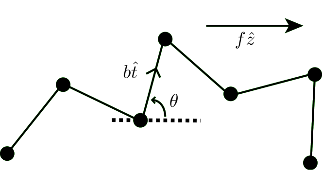
Figure 1: The Freely Jointed Chain consists of identical segments of length $b$, joined together by free hinges. The configuration is fully described by the collection of orientation vectors $\{\hat{t}_{i}\}$. $\{\theta_{i}\}$ denotes the angle between $\hat{t}_{i}$ and the fixed direction $\hat{z}$ of the applied stretching force.

To formulate the FJC we describe a molecular conformation by associating with each segment a unit orientation vector $\hat{t}_{i}$, pointing in the direction of the $i$th segment, as sketched in Fig. 1. In the presence of an external force $\vec{f}$ along the $\hat{z}$ direction, we can define an energy functional for the chain

$$\frac{{\cal E}^{{\mathrm{FJC}}}[\hat{t}_{i}]}{{k_{\rm B}}T}=-\sum_{i=1}^{N}\frac{fb}{{k_{\rm B}}T}\,\hat{t}_{i}\cdot\hat{z}\,.$$ (1)

In the absence of an external force, all configurations have equal energy and (neglecting self-avoidance) the chain displays the characteristics of a random walk. To pull the ends of such a chain away from each other a force has to be applied, as extending the chain reduces its conformational entropy. The resulting entropic elastic behavior can be summarized in the force-extension relation Grosberg and Khlokhlov (1994)

$$\langle\frac{z}{L_{\text{tot}}}\rangle=\coth(\frac{fb}{{k_{\rm B}}T})-\frac{{k_{\rm B}}T}{fb}\,,$$ (2)

the well-known Langevin function. In the limit of low stretching force, all polymer models reduce to Hooke-law behavior $f=k_{\rm sp}\langle z\rangle$; we define the effective spring constant by $\kappa=k_{\rm sp}\cdot L_{\mathrm{tot}}$, or

$$\langle\frac{z}{L_{\mathrm{tot}}}\rangle\to\frac{f}{\kappa}+{\cal O}(f^{2})\,.$$ (3)

Expanding Eq. 2 gives the effective spring constant for the FJC as $\kappa^{\text{FJC}}=\tfrac{3{k_{\rm B}T}}{b}$. The fact that the effective spring constant is proportional to the absolute temperature illustrates that the elasticity in this model is purely entropic in nature.

At high stretching force, Eq. 2 gives $\langle\frac{z}{L_{\mathrm{tot}}}\rangle\to 1$; the extension saturates when all the links of the chain are aligned by the external force. In reality, individual links are slightly extensible; we will modify the model to introduce this effect in Sect. II.3.

II.2 The Wormlike Chain

As mentioned above, double-stranded DNA (dsDNA) is far from being a freely jointed chain. Thus it is unsurprising that while the FJC model can reproduce the observed linear force-extension relation of dsDNA at low stretching force, and the observed saturation at high force, still it fails at intermediate values of $f$. Another indication that the model is physically inappropriate is that the best-fit value of the link length is $b\approx 100\,$nm, completely different from the physical contour length per basepair of $0.34\,$nm.

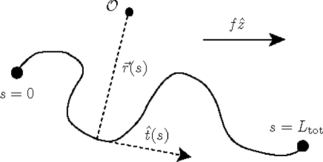
Figure 2: A Worm Like Chain is a continuum elastic medium, whose configuration is described in terms of the position vector $\vec{r}$ as a function of the contour length $s$.

To improve upon the FJC, we must account for the fact that the monomers do resist bending. In fact, the very great stiffness of double-stranded DNA can be turned to our advantage, as it implies that successive monomers are constrained to point in nearly the same direction. Thus we can treat the polymer as a continuum elastic body, its configuration described by the position $\vec{r}(s)$ as a function of the relaxed-state contour length $s$ (see Fig. 2). Continuing to treat the chain as inextensible gives the Worm Like Chain Kratky and Porod (1949); Saito et al. (1967). The local tangent and curvature vectors ($\vec{t}$ and $\vec{w}$, respectively) are given by

$$\vec{t}(s)=\frac{{\rm d}\vec{r}(s)}{{\rm d}s}\,,\quad\vec{w}(s)=\frac{{\rm d}\vec{t}(s)}{{\rm d}s}\,.$$ (4)

We temporarily assume that the chain is inextensible, expressed locally by the condition that $|\vec{t}(s)|=1$ everywhere.

To get an energy functional generalizing Eq. 1, we note that for a thin, homogeneous rod the energy density of elastic strain is proportional to the square of the local curvature. Adding the external-force term from Eq. 1 yields

$$\frac{{\cal E}^{{\mathrm{WLC}}}[\hat{t}(s)]}{{k_{\rm B}}T}=\int_{0}^{L_{\text{tot}}}{\rm d}s\left\{\frac{A}{2}\left|\frac{{\rm d}\hat{t}(s)}{{\rm d}s}\right|^{2}-\frac{f}{{k_{\rm B}}T}\hat{t}(s)\cdot\hat{z}\right\}\,.$$ (5)

Eq. 5 makes it clear that the parameter $A$ is a measure of the bend stiffness of the chain. $A$ is also the persistence length of the chain, the characteristic length scale associated with the decay of tangent-tangent correlations at zero stretching force:

$$\langle\hat{t}(0)\cdot\hat{t}(s)\rangle_{\text{WLC}}\sim e^{-|s|/A}\,.$$ (6)

The force-extension relation for the WLC was obtained numerically in Marko and Siggia (1995); subsequently a high-precision interpolation formula was given in Bouchiat et al. (1999). At low force, the WLC also behaves like an ideal spring, with effective spring constant Yamakawa (1971)

$$\kappa^{\text{WLC}}=\frac{3{k_{\rm B}}T}{2A}\,.$$ (7)

Thus a WLC with stiffness parameter $A$ yields a force-extension relation that at low force matches the FJC with $b=2A$.

The remarks at the start of this subsection make it clear that the WLC is just an approximation, valid in the limit where the persistence length $A$ is much longer than the physical monomer length (and width). When these conditions are not met, the picture of the molecule as a thin, continuous, elastic body will not be accurate; short-length cutoff effects will then enter in an essential way.

II.3 Experiments

Early single-molecule stretching experiments showed that double-stranded DNA closely follows the predicted force-extension of the WLC at forces under $10\,$pN Bustamante et al. (1994). Later experiments probing the region $10\,\mathrm{pN}<f<60\,\mathrm{pN}$ found a linear deviation from the WLC prediction, attributable to a Hooke-law stretching elasticity Cluzel et al. (1996); Smith et al. (1996); Wang et al. (1997). Adding this effect into the model introduces a second fit parameter $E$ in addition to $A$. To lowest order in $f/E$ this modification just amounts to multiplying the model’s $\langle\frac{z}{L_{\mathrm{tot}}}\rangle$ by the factor $(1+\tfrac{f}{E})$; for dsDNA the resulting fit is very good out to $60\,\mathrm{pN}$.

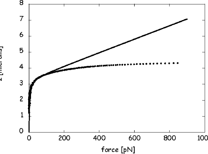
Figure 5: Least-squares fit (solid line) of the single-stranded DNA stretching data (closed circles) from Rief et al. (1999) to the extensible FJC model. Included in the fit are the data up to a force of 100 pN. Fitting only those data points yields a link length $b=1.75\,$nm and a stretch modulus $E=8\cdot 10^{2}\,\mathrm{pN}$, reproducing the typical values as cited for instance in Rief et al. (1999); Clausen-Schaumann et al. (2000); Hegner et al. (1999). In this graph, we have extrapolated this fit to the high-force range, to demonstrate that the parameters as extracted from the low-force data do not represent the full range of data faithfully.

The situation for single-stranded DNA has been less clear. Adding an extensibility factor to Eq. 2 again yields a model with two parameters ($b$ and $E$). Though this “extensible FJC” (EFJC) model yielded impressive fits to the early experimental data, recent advances in single-molecule manipulation Rief et al. (1999); Clausen-Schaumann et al. (2000) have again probed higher forces, and here the agreement is not so good. As shown in Fig. 5, the previously cited values for $b$ and $E$ do not give a successful extrapolation to the regime of higher forces. In the following section, we will propose a new model that borrows features from both the FJC and the WLC to describe these data more accurately.

III The Discrete Persistent Chain

The previous sections have made it clear that a real polymer will display both discreteness and bend stiffness. While we have seen that the corresponding effects on the force-extension relation are interchangeable at very low forces, higher forces will distinguish them. Accordingly we now formulate a model with both $b$ and $A$; later we will add a stretch stiffness as well.

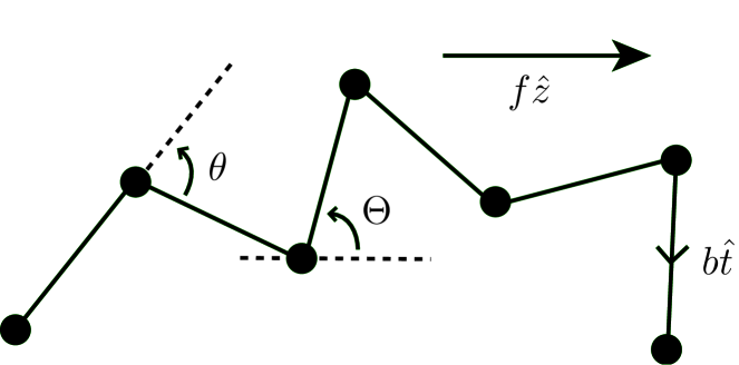
Figure 3: The Discrete Persistent Chain, viewed as a FJC with an additional term in the energy proportional to the square of the polar angle $\Theta$ between successive segments.

Our “Discrete Persistent Chain” (or DPC) models the polymer as a chain composed of $N$ segments of length $b$, whose conformation is once again fully described by the collection of orientation vectors $\{\hat{t}_{i}\}$ (see Fig. 3). Bend resistance is taken into account by including an energy penalty at each link proportional to the square of the angle ($\Theta_{i,i+1}=\arccos\hat{t}_{i}\cdot\hat{t}_{i+1}$) between two subsequent links. The energy functional describing this model is thus given by

$$\frac{{\cal E}^{{\mathrm{DPC}}}[\{\hat{t}_{i}\}]}{{k_{\rm B}}T}=-\sum_{i=1}^{N}\frac{fb}{{k_{\rm B}}T}\,\hat{t}_{i}\cdot\hat{z}\,+\sum_{i=1}^{N-1}\frac{A}{2b}(\Theta_{i,i+1})^{2}\,.$$ (8)

The partition function for this energy functional is then given by

$${\cal Z}=\left[\prod_{i=1}^{N}\int_{{\mathbb{S}}^{2}}\!{\rm d}^{2}\hat{t}_{i}\!\right]e^{-\frac{fb}{2{k_{\rm B}}T}\hat{t}_{1}\cdot\hat{z}}\left\{\prod_{i=1}^{N-1}e^{-{\cal E}_{i}(\hat{t}_{i},\hat{t}_{i+1})/{k_{\rm B}}T}\right\}e^{-\frac{fb}{2{k_{\rm B}}T}\hat{t}_{N}\cdot\hat{z}}\,,$$ (9)

where

$$\frac{{\cal E}_{i}(\hat{t}_{i},\hat{t}_{i+1})}{{k_{\rm B}}T}=-\frac{fb}{2{k_{\rm B}}T}\,(\hat{t}_{i}+\hat{t}_{i+1})\cdot\hat{z}\,+\frac{A}{2b}(\Theta_{i,i+1})^{2}$$ (10)

and ${\mathbb{S}}^{2}$ is the two-dimensional unit sphere.

To compute ${\cal Z}$ we interpret each integral in Eq. 9 as a generalized matrix product (among matrices with continuous indices), writing Kramers and Wannier (1941)

$${\cal Z}=\vec{v}\cdot{\sf T}^{N-1}\cdot\vec{w}\,.$$ (11)

In this formula $\vec{v}$ and $\vec{w}$ are vectors indexed by $\hat{t}$, or in other words functions $v(\hat{t}\,),w(\hat{t}\,)$. The matrix product ${\sf T}\cdot\vec{v}$ is a new vector, defined by the convolution:

$$({\sf T}\cdot\vec{v}\,)(\hat{t}_{i})=\int_{{\mathbb{S}}^{2}}\!{\rm d}^{2}\hat{t}_{j}\,{\mathbb{T}}(\hat{t}_{i},\hat{t}_{j})v(\hat{t}_{j})\,.$$ (12)

The matrix elements of ${\sf T}$ are given by

$${\mathbb{T}}(\hat{t}_{i},\hat{t}_{j})=e^{-{\cal E}_{i}(\hat{t}_{i},\hat{t}_{j})/{k_{\rm B}}T}\,;$$ (13)

we will not need the explicit forms of $\vec{v}$ and $\vec{w}$ below.

The force-extension relation can be obtained from ${\cal Z}$ by differentiating with respect to the force (see Eqs. 9–10):

$$\langle\frac{z}{L_{\text{tot}}}\rangle=\left(\frac{{k_{\rm B}}T}{L_{\text{tot}}}\right)\frac{\rm d}{{\rm d}f}\ln{\cal Z}\,.$$ (14)

It is here that the transfer matrix formulation can be used to greatly simplify the calculation of the force-extension relation, since all that is needed to compute the logarithmic derivative of ${\cal Z}$ in the limit of long chains is the largest eigenvalue of ${\sf T}$, which we will call $\lambda_{\text{max}}$:

$$\langle\frac{z}{L_{\text{tot}}}\rangle\stackrel{{\scriptstyle\mathrm{large}N}}{{\longrightarrow}}\left(\frac{{k_{\rm B}}T}{L_{\text{tot}}}\right)\frac{\rm d}{{\rm d}f}\ln(\lambda_{\max})^{N}=\left(\frac{{k_{\rm B}}T}{b}\right)\frac{\rm d}{{\rm d}f}\ln{\lambda_{\max}}\,.$$ (15)

We will approximate $\lambda_{\text{max}}$ using a variational scheme. Following the line of argument of Marko and Siggia (1995), we note that the leading eigenfunction of ${\sf T}$ will reflect the physics of the problem in the sense that it must be azimuthally symmetric and peaked in the direction of the applied force. A suitable 1-parameter family of trial eigenfunctions $\vec{v}_{\omega}$ can therefore be defined by

$$v_{\omega}(\hat{t}\,)=e^{\omega\hat{t}\cdot\hat{z}}\,.$$ (16)

Under (12), the $\vec{v}_{\omega}$ have squared norms

$$\|\vec{v}_{\omega}\|^{2}=\tfrac{2\pi}{\omega}\sinh(2\omega)\,,$$ (17)

which allows us to approximate $\lambda_{\text{max}}$ variationally by

$$\lambda_{\text{max}}^{*}\equiv\max_{\omega}y(\omega)\equiv\max_{\omega}\,\frac{\vec{v}_{\omega}\cdot{\sf T}\cdot\vec{v}_{\omega}}{\|\vec{v}_{\omega}\|^{2}}\,.$$ (18)

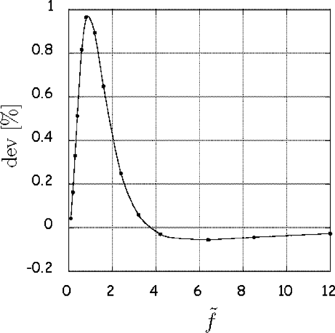
Figure 4: Comparison between the exact WLC force-extension solution and the Ritz variational approximation. The deviation ${\rm dev}(\tilde{f})$ is defined as $100\%\times(z(\tilde{f})_{\rm exact}\!-\!z(\tilde{f})_{\rm var})/z(\tilde{f})_{\rm exact}$, with $\tilde{f}$ the dimensionless force $\tilde{f}=\frac{fA}{{k_{\rm B}}T}$. The maximal error induced by the variational approximation is about $1\%$. Data for the exact solution were taken from Bouchiat et al. (1999).

To get some idea of the quality of this variational approach, we can compare its results in the limit $b\to 0$ (the WLC) to the exact solution of that model. Fig. 4 plots the difference of these force-extension curves, and shows that the results from the variational approximation are nowhere off by more than $1\%$.

Returning to the full DPC model, Appendix A shows that it is possible to express $y(\omega)$ in terms of the dimensionless variables

$$\tilde{f}=\frac{fb}{{k_{\rm B}}T}\,,\qquad\tilde{\ell}=\frac{A}{b}$$ (19)

as a combination of error functions as follows

$$y(\omega) = \frac{2\sqrt{2}\pi^{3/2}\omega e^{-2\tilde{\ell}-\frac{(2\omega+\tilde{f})^{2}}{8\tilde{\ell}}}\text{csch}(2\omega)}{\sqrt{-\tilde{\ell}}(2\omega+\tilde{f})}\times$$ (20)

$$\times\left[\text{Erf}\left(\frac{i}{2\sqrt{2\tilde{\ell}}}(\tilde{f}+4\tilde{\ell}+2\omega)\right)-\text{Erf}\left(\frac{i}{2\sqrt{2\tilde{\ell}}}(\tilde{f}-4\tilde{\ell}+2\omega)\right)\right]\,.$$

This formula is only valid in the parameter regime where $\omega^{*}$ (the locus of the maximum of Eq. 20) obeys

$$\omega^{*}>\tilde{\ell}-\frac{1}{2}\tilde{f}\,.$$ (21)

For practical purposes this is the region where the magnitude of the bend stiffness $A$ is larger than, or at most comparable to, the link length $b$, which is the physically relevant regime. We maximize Eq. 20 numerically to obtain $\lambda_{\text{max}}^{*}$, from which we can then compute the force-extension relation by numerical differentiation with respect to the force. In the small force limit, we can do a little better based on the observation that for small $\tilde{f}$, $\omega^{*}$ is also small. Expanding Eq. 20 to second order in $\omega$ and $\tilde{f}$ we can analytically solve the stationarity condition $\frac{{\rm d}y}{{\rm d}\omega}=0$ (which is now simply a quadratic equation) and determine the small force entropic elastic behavior of our DPC model to be

$$\langle\frac{z}{L_{\text{tot}}}\rangle\to\frac{f}{\kappa^{{\mathrm{DPC}}}}+{\cal O}(f^{2})\,,$$ (22)

where the effective spring constant for the DPC model is given by

$$\kappa^{{\mathrm{DPC}}}=\frac{3}{2}\frac{{k_{\rm B}T}}{A}\left(1-\frac{b}{2A}\right)^{\raise 0.45206pt\hbox{${\scriptscriptstyle-}$}\kern-0.35002pt1}\,.$$ (23)

It is sometimes convenient to reexpress the parameters $A$ and $b$ of the DPC model in terms of $\kappa^{{\mathrm{DPC}}}$ and $b$. We do this using Eq. 23:

$$A=\frac{b}{2}+\frac{3{k_{\rm B}}T}{2\kappa^{{\mathrm{DPC}}}}\,.$$ (24)

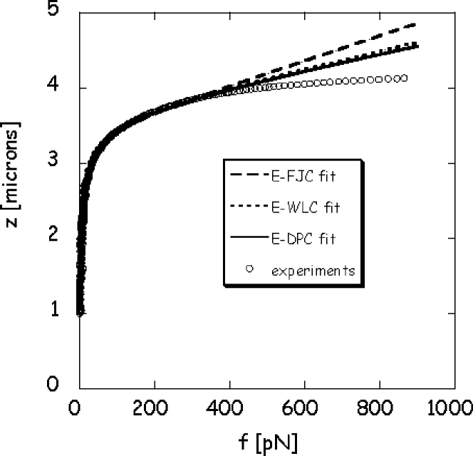
Figure 6: Fit of the extensible DPC model (solid line) to the single-strand DNA stretching data (circles) kindly supplied by M. Rief; see Rief et al. (1999). The fit shown was obtained for $b=0.17\,,E=4.5\cdot 10^{3}\,\mathrm{pN}\,,L_{\rm tot}=3.9\,\mu$m, and $\kappa^{{\mathrm{DPC}}}=\frac{3}{2}\frac{{k_{\rm B}T}}{0.85\,\mathrm{nm}}$. In addition, the dashed and dotted lines show the corresponding best fits to the extensible FJC and WLC, respectively. All fits include the data points only for forces between 20 pN and 400 pN. Values for $\chi^{2}$ were EFJC : $\chi^{2}=1.269$; EWLC : $\chi^{2}=0.600$ and EDPC : $\chi^{2}=0.490$ at $N=1523$. We ignore the lowest-force points because of complications induced by hairpins and other secondary structures in the DNA.

It is straightforward to add an intrinsic stretch modulus to the calculation outlined above, obtaining the “Extensible DPC” (or EDPC) model. We have computed the resulting force-extension curves, and fitted to recent data for ssDNA. The results of these fits are collected in Fig. 6. Fitting to the data points with $f<400\,$pN yields a value of the stretch modulus of around $E\approx 4500\,\mathrm{pN}$, more than four times larger than even the largest of the previous estimates Rief et al. (1999); Clausen-Schaumann et al. (2000); Hegner et al. (1999). We interpret this discrepancy by noting that if we hold $\kappa$ constant while varying $b$, the difference between the EFJC and EDPC models shows up in the high-force regime, which is also sensitive to the choice of $E$. Thus neglecting cutoff effects causes curve fitting to make a compensating change in $E$.

The best fit (in terms of $\chi^{2}$) is obtained for a value of $b\approx 0.17\,$nm, away from both the EWLC ($b=0$) and EFJC ($b=\tfrac{3{k_{\rm B}}T}{\kappa}=1.7\,$nm) limits of the model. Even though to the eye the difference between the three models in the fit region might appear marginal, the improvement in $\chi^{2}$ achieved by the DPC at just over $18\%$ is statistically relevant. Interestingly, the fit value of $b$ is indeed comparable to the physical segment length of ssDNA ($0.6\,$nm), a result not put in by hand. Fig. 6 also shows that our EDPC model extrapolates better to the high-force regime than either the EFJC or the EWLC.

Previous authors have already noted that the extensible FJC model does not accurately model the high-force data Rief et al. (1999); Clausen-Schaumann et al. (2000), but have attributed its failure to the onset of nonlinear elasticity effects. We may expect such effects to become significant when the ratio $f/E$ exceeds, say, 10%. Our large fit value of $E$ means that we ought to be able to trust our linear-elasticity model out to around $f=400\,\mathrm{pN}$, which is why we used only the data up to this point in our fit. Indeed Fig. 6 shows that the extensible DPC model works well out to $f=400\,\mathrm{pN}$. Carrying the fit out to still larger values of $f$ would raise the fit value of $E$ still further.

IV The Overstretching Transition

IV.1 Background

As first observed by Cluzel et el. Cluzel et al. (1996) and Smith et al Smith et al. (1996), stretching double stranded DNA is quite different from single-strand DNA. Their experiments showed that at a force of around 65–70 pN the DNA sample suddenly snaps open (an “overstretching transition”), extending to almost twice its original contour length before entering a second entropic stretching regime. This second regime clearly represents a “stretched” DNA configuration quite different from ordinary double stranded or B-DNA, and has been dubbed S-DNA. The transition from B-DNA into S-DNA is very sharp, indicating a high level of cooperativity.

S-DNA appears to have a definite helical pitch Léger et al. (1999); Léger (1999), consistent with its being a new, double-stranded conformation. An alternative view interprets the overstretching transition as force-induced melting (denaturation) of the B-DNA duplex Rouzina and Bloomfield (2001a, b). One implication of the latter view is that S-DNA should have elastic properties similar to those of two single strands, a point to which we will return later.

Whatever view we take of its structural character, the sharpness of the overstretching transition is reminiscent of another well-studied structural transition in biopolymers, the helix-coil transition Zimm and Bragg (1959). Inspired by the classic analysis of Zimm and Bragg, this section will model the B$\to$S transition by a two-state (Ising) model living on a DPC (the “Ising–DPC model”). We will make no assumptions about the nature of either B- or S-DNA. Both are allowed to have arbitrary bend and stretch stiffnesses. Our aim is to fit the resulting force-extension curves to the available data and to see whether the values of the elastic constants can help characterize the stretched state. (The other state is just double stranded DNA, whose elastic constants are well known.)

IV.2 General Setup

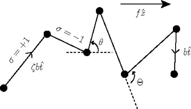
Figure 7: Conventions for the Ising-DPC model. We take $\sigma=+1$ to correspond to B-DNA, and $\sigma=-1$ to S-DNA. Each segment of S-DNA is longer than B-DNA by a factor $\zeta$. Definitions of $\hat{t},\theta$ and $\Theta$ are the same as before.

Fig. 7 illustrates the model that we will be considering in some more detail. We envision a chain consisting of N links, connected by hinges that try to align the segments they join. Each segment carries a discrete variable $\sigma$, which takes the values $\pm 1$. We will take $\sigma=+1$ to mean the segment is in the B-state and $\sigma=-1$ for the S-state. The factor by which a segment elongates when going from B to S will be called $\zeta$, i.e. $b^{S}=\zeta b$ (with $\zeta>1$). We assign a bend stiffness parameter $A$ to B-DNA, and a different $A^{S}\equiv\beta\zeta A$ to S-DNA; $\beta$ is a dimensionless parameter with $\beta\zeta<1$. We also need to assign a bend stiffness to a hinge joining a B and an S segment. This value we will call $\eta A$.

We can now write down the full energy functional for our Ising-DPC model:

$$\frac{{\cal E}[\{\hat{t}_{i},\sigma_{i}\}]}{{k_{\rm B}}T} = -\sum_{i=1}^{N-1}\biggl{\{}\frac{\alpha_{0}}{2}(\sigma_{i}\!+\!\sigma_{i+\!1})+\gamma(\sigma_{i}\sigma_{i+\!1}\!-\!1)+$$ (25)

$$+\frac{fb}{2{k_{\rm B}}T}\left[(\frac{1\!+\!\sigma_{i}}{2}\!+\!\frac{1\!-\!\sigma_{i}}{2}\zeta)\hat{t}_{i}\cdot\hat{z}\!+\!(\frac{1\!+\!\sigma_{i+\!1}}{2}\!+\!\frac{1\!-\!\sigma_{i+\!1}}{2}\zeta)\hat{t}_{i+\!1}\cdot\hat{z}\right]\!-$$

$$-\frac{A}{2b}\left[\frac{(1\!-\!\sigma_{i})(1\!-\!\sigma_{i+\!1})}{4}\beta+|\sigma_{i}\!-\!\sigma_{i+\!1}|\eta+\frac{(1\!+\!\sigma_{i})(1\!+\!\sigma_{i+\!1})}{4}\right](\Theta_{i,i+\!1})^{2}\biggr{\}}\,.$$

The first line is the pure-Ising part, with $2\alpha_{0}{k_{\rm B}}T$ the intrinsic free energy cost of converting a single segment from B to S and $2\gamma{k_{\rm B}}T$ the energy cost of creating a B$\to$S interface. Note that we ignore a contribution to the energy functional from the first and last segments. In the long-chain limit this does not affect the outcome of our calculation.

The partition function for the energy functional (25), ${\cal E}[\{\hat{t}_{i},\sigma_{i}\}]=\sum_{i=1}^{N-1}{\cal E}_{i}(\hat{t}_{i},\sigma_{i},\hat{t}_{i+1},\sigma_{i+1})$, is given by

$${\cal Z}=\left[\prod_{i=1}^{N-1}\sum_{\sigma_{i}=\pm 1}\!\int_{{\mathbb{S}}^{2}}\!{\rm d}^{2}\hat{t}_{i}\right]\!\prod_{i=1}^{N-1}e^{-{\cal E}_{i}(\hat{t}_{i},\sigma_{i},\hat{t}_{i+1},\sigma_{i+1})/{k_{\rm B}}T}\,.$$ (26)

We will again calculate ${\cal Z}$ with the aid of the transfer matrix technique Kramers and Wannier (1941), writing Eq. 26 as

$${\cal Z}=\vec{v}\cdot{\sf T}^{N-1}\cdot\vec{w}\,,$$ (27)

with ${\sf T}$ now the transfer matrix for our Ising-DPC model, which carries an additional 2-by-2 structure due to the Ising variables. The dot products are thus defined as

$$({\sf T}\cdot\vec{v})_{\sigma_{i}}(\hat{t}_{i})=\sum_{\sigma_{j}=\pm 1}\!\int_{{\mathbb{S}}^{2}}\!{\rm d}^{2}\hat{t}_{j}\,{\mathbb{T}}_{\sigma_{i}\sigma_{j}}(\hat{t}_{i},\hat{t}_{j})v_{\sigma_{j}}(\hat{t}_{j})\,.$$ (28)

The individual matrix elements ${\mathbb{T}}_{\sigma_{i}\sigma_{j}}$ are given explicitly by

$${\mathbb{T}}_{1,1}(\hat{t}_{i},\hat{t}_{i+1}) = \exp\left[\frac{1}{2}\tilde{f}(\hat{t}_{i}\!+\!\hat{t}_{i+1})\cdot\hat{z}\!-\!\frac{A}{b}(1\!-\!\hat{t}_{i}\cdot\hat{t}_{i+1})+\alpha_{0}\right]$$

$${\mathbb{T}}_{1,\!-\!1}(\hat{t}_{i},\hat{t}_{i+1}) = \exp\left[\frac{1}{2}\tilde{f}(\hat{t}_{i}\!+\!\zeta\hat{t}_{i+1})\cdot\hat{z}\!-\!\frac{\eta A}{b}(1\!-\!\hat{t}_{i}\cdot\hat{t}_{i+1})\!-\!2\gamma\right]$$

$${\mathbb{T}}_{-1,1}(\hat{t}_{i},\hat{t}_{i+1}) = \exp\left[\frac{1}{2}\tilde{f}(\zeta\hat{t}_{i}\!+\!\hat{t}_{i+1})\cdot\hat{z}\!-\!\frac{\eta A}{b}(1\!-\!\hat{t}_{i}\cdot\hat{t}_{i+1})\!-\!2\gamma\right]$$

$${\mathbb{T}}_{-1,-1}(\hat{t}_{i},\hat{t}_{i+1}) = \exp\left[\frac{1}{2}\zeta\tilde{f}(\hat{t}_{i}\!+\!\hat{t}_{i+1})\cdot\hat{z}\!-\!\frac{\beta A}{b}(1\!-\!\hat{t}_{i}\cdot\hat{t}_{i+1})\!-\!\alpha_{0}\right]\,,$$

where again $\tilde{f}\equiv\frac{fb}{{k_{\rm B}}T}$.

Once again we approximate the largest eigenvalue of the transfer matrix ${\sf T}$ using a variational approach, choosing our trial eigenfunctions to possess azimuthal symmetry and to be peaked in the direction of the force $\hat{z}$. This time, however, we need a three-parameter family of trial functions:

$$v_{\omega_{1},\omega_{-1},\varphi}(\hat{t}\,)=\left(\begin{array}[]{c }\left(\frac{\omega_{1}}{\sinh(2\omega_{1})}\right)^{\frac{1}{2}}e^{\omega_{1}\hat{t}\cdot\hat{z}}\cos\varphi\\ \left(\frac{\omega_{-1}}{\sinh(2\omega_{-1})}\right)^{\frac{1}{2}}e^{\omega_{-1}\hat{t}\cdot\hat{z}}\sin\varphi\end{array}\right)\,,$$ (29)

chosen such that their squared norm is independent of all parameters

$$\|\vec{v}_{\omega_{1},\omega_{-1},\varphi}\|^{2}=2\pi\,.$$ (30)

Eq. 29 shows that once again the $\omega$’s gives the degree of alignment of the monomers (how forward-peaked their probability distribution is), whereas $\varphi$ describes the relative probability of a monomer to be in the two states. The variational estimate for the maximal eigenvalue is now given by

$$\lambda^{*}_{\text{max}}\equiv\max_{\omega_{1},\omega_{-1},\varphi}y(\omega,\varphi)\equiv\max_{\omega_{1},\omega_{-1},\varphi}\,\frac{\vec{v}_{\omega_{1},\omega_{-1},\varphi}\cdot{\sf T}\cdot\vec{v}_{\omega_{1},\omega_{-1},\varphi}}{\|\vec{v}_{\omega_{1},\omega_{-1},\varphi}\|^{2}}\,,$$ (31)

The maximization over $\varphi$ can be done analytically: defining the $2\times 2$ matrix $\tilde{\sf T}(\omega_{1},\omega_{-1})$ by

$$\vec{v}_{\omega_{1},\omega_{-1},\varphi}\cdot{\sf T}\cdot\vec{v}_{\omega_{1},\omega_{-1},\varphi}=(\cos\varphi,\sin\varphi)\cdot\tilde{\sf T}(\omega_{1},\omega_{-1})\cdot\left(\begin{array}[]{c }\cos\varphi\\ \,\sin\varphi\end{array}\right)\,,$$ (32)

or equivalently specifying its entries

$$\tilde{\mathbb{T}}_{\sigma_{i}\sigma_{j}}(\omega_{\sigma_{i}},\omega_{\sigma_{j}})=\int_{{\mathbb{S}}^{2}}\!{\rm d}^{2}\hat{t}_{i}\int_{{\mathbb{S}}^{2}}\!{\rm d}^{2}\hat{t}_{j}\,\left(\frac{\omega_{\sigma_{i}}}{\sinh(2\omega_{\sigma_{i}})}\right)^{\frac{1}{2}}e^{\omega_{\sigma_{i}}\hat{t}_{i}\cdot\hat{z}}\,{\mathbb{T}}_{\sigma_{i}\sigma_{j}}(\hat{t}_{i},\hat{t}_{j})\left(\frac{\omega_{\sigma_{j}}}{\sinh(2\omega_{\sigma_{j}})}\right)^{\frac{1}{2}}e^{\omega_{\sigma_{j}}\hat{t}_{j}\cdot\hat{z}}\,,$$ (33)

it is easy to show that

$$\lambda^{*}_{\text{max}}=\max_{\omega_{1},\omega_{-1}}\,\frac{\tilde{y}(\omega_{1},\omega_{-1})}{\|\vec{v}_{\omega_{1},\omega_{-1},\varphi}\|^{2}}\,,$$ (34)

where $\tilde{y}(\omega_{1},\omega_{-1})$ is the maximal eigenvalue of $\tilde{\sf T}(\omega_{1},\omega_{-1})$. The following subsection will calculate this eigenvalue in a continuum approximation to $\tilde{\sf T}(\omega_{1},\omega_{-1})$, illustrating the procedure by considering in some detail the matrix element $\tilde{\mathbb{T}}_{1,1}(\omega_{1},\omega_{-1})$. The other matrix elements can be obtained analogously. Writing out the integrals explicitly, we have

$$\tilde{\mathbb{T}}_{1,1}(\omega_{1})=\frac{\omega_{1}e^{\alpha_{0}-\frac{A}{b}}}{\sinh(2\omega_{1})}\int_{{\mathbb{S}}^{2}}\!{\rm d}^{2}\hat{t}_{i}e^{\hat{a}\hat{t}_{i}\cdot\hat{z}}\int_{{\mathbb{S}}^{2}}\!{\rm d}^{2}\hat{t}_{i+1}\left[e^{(\hat{a}\hat{z}+\frac{A}{b}\hat{t}_{i})\cdot\hat{t}_{i+1}}\right]\,,$$ (35)

where we have introduced $\hat{a}\equiv\omega_{1}+\frac{\tilde{f}}{2}$. Condensing notation even further we define $\mu^{2}=\hat{a}^{2}+(\tfrac{A}{b})^{2}+2\hat{a}\tfrac{A}{b}\hat{t}_{i}\cdot\hat{z}$, which allows us to write

$$\tilde{\mathbb{T}}_{1,1}(\omega_{1})\!=\!(2\pi)^{2}\frac{\omega_{1}e^{\alpha_{0}-\frac{A}{b}}}{\sinh(2\omega_{1})}\int_{|\tfrac{A}{b}\!-\!\hat{a}|}^{\tfrac{A}{b}\!+\hat{a}}\!\!\ \frac{b\,{\rm d}\mu}{\hat{a}A}e^{\frac{b}{2A}(\mu^{2}\!-\!\hat{a}^{2}\!-\!(\frac{A}{b})^{2})}\left[e^{\mu}\!-\!e^{-\mu}\right]\,.$$ (36)

IV.3 Continuum Limit

We could now proceed to evaluate the force-extension relation of the Ising-DPC model, by generalizing Sect. III. To simplify the calculations, however, we will first pass to a continuum limit. To justify this step, note that Fig. 6 shows that the continuum (WLC) approximation gives an excellent account of single-stranded DNA stretching out to forces beyond those probed in overstretching experiments (about $90\,\mathrm{pN}$). As mentioned earlier, the continuum approximation is also quite good for double-stranded DNA, because the latter’s persistence length is so much longer than its monomer size.

In the continuum limit $b$ is sent to zero holding $L_{\mathrm{tot}}$ fixed; hence $N\to\infty$. The bookkeeping is more manageable after a shift in $\mu$:

$$x\equiv\mu-\frac{A}{b}\,.$$ (37)

Eq. 36 then reduces to

$$\tilde{\mathbb{T}}_{1,1}(\omega_{1})\! = \!\frac{\omega_{1}e^{\alpha_{0}}}{\sinh(2\omega_{1})}\frac{(2\pi)^{2}b}{\hat{a}A}\int_{-\hat{a}}^{+\hat{a}}\!\!\,{\rm d}x\,\exp\left[\frac{b}{2A}x^{2}+2x-\frac{\hat{a}^{2}b}{2A}\right]$$ (38)

$$\approx \!\frac{\omega_{1}e^{\alpha_{0}}}{\sinh(2\omega_{1})}\frac{(2\pi)^{2}b}{\hat{a}A}\int_{-\hat{a}}^{+\hat{a}}\!\!\,{\rm d}x\,e^{2x}(1+\frac{x^{2}b}{2A})e^{-\frac{\hat{a}^{2}b}{2A}}\,.$$

The last integral can be worked out exactly, and expanding the result to second order in $b$ we end up with

$$\frac{A}{2\pi b}\frac{1}{\|\vec{v}_{\omega_{1},\omega_{-1},\varphi}\|^{2}}\tilde{\mathbb{T}}_{1,1}(\omega_{1})\!=\!e^{\alpha_{0}}\left[1+{b}\left(\frac{f}{{k_{\rm B}}T}-\frac{\omega_{1}}{2A}\right)\left(\coth(2\omega_{1})-\frac{1}{2\omega_{1}}\right)\right]\,.$$ (39)

In similar fashion, we can obtain the following expressions for the other matrix elements.

$$\frac{A}{2\pi b}\frac{1}{\|\vec{v}_{\omega_{1},\omega_{-1},\varphi}\|^{2}}\tilde{\mathbb{T}}_{-1,-1}(\omega_{-1})\! = \!\beta^{\raise 0.45206pt\hbox{${\scriptscriptstyle-}$}\kern-0.35002pt1}e^{-\alpha_{0}}\left[1+{b}\left(\frac{\zeta f}{{k_{\rm B}}T}-\frac{\omega_{-1}}{2\beta A}\right)\left(\coth(2\omega_{-1})-\frac{1}{2\omega_{-1}}\right)\right]$$

$$\frac{A}{2\pi b}\frac{1}{\|\vec{v}_{\omega_{1},\omega_{-1},\varphi}\|^{2}}\tilde{\mathbb{T}}_{1,-1}(\omega_{1},\omega_{-1})\! = \!\frac{e^{-2\gamma}}{\eta}\left(\frac{\omega_{1}\omega_{-1}}{\sinh(2\omega_{1})\sinh(2\omega_{-1})}\right)^{\frac{1}{2}}\left(\frac{2\sinh(\omega_{1}+\omega_{-1})}{\omega_{1}+\omega_{-1}}\right)\,.$$ (40)

To obtain a nontrivial continuum limit we must now specify how the parameters $A$, $\alpha_{0}$, and $\gamma$ depend on $b$ as $b\to 0$. It is straightforward to show that the choices

$$\alpha_{0}=-\frac{1}{2}\ln\beta+b\bar{\alpha}\,,\qquad\gamma=-\frac{1}{2}\ln(\bar{g}b)$$ (41)

work, where we hold $A$, $\bar{\alpha}$, $\beta$ and $\bar{g}$ fixed as $b\to 0$. With these choices, the matrix $\frac{1}{\|\vec{v}_{\omega_{1},\omega_{-1},\varphi}\|^{2}}\tilde{\sf T}(\omega_{1},\omega_{-1})$ takes the form

$$\frac{1}{\|\vec{v}_{\omega_{1},\omega_{-1},\varphi}\|^{2}}\tilde{\sf T}(\omega_{1},\omega_{-1})=\frac{2\pi b}{A\sqrt{\beta}}\left(\openone+b\begin{pmatrix}{\cal P}&{\cal Q}\\ {\cal Q}&{\cal R}\end{pmatrix}\right)\,,$$ (42)

with

$${\cal P} = \bar{\alpha}+\left(\frac{f}{{k_{\rm B}}T}-\frac{\omega_{1}}{2A}\right)\left(\coth(2\omega_{1})-\frac{1}{2\omega_{1}}\right)\,,$$

$${\cal R} = -\bar{\alpha}+\left(\frac{\zeta f}{{k_{\rm B}}T}-\frac{\omega_{-1}}{2A\beta}\right)\left(\coth(2\omega_{-1})-\frac{1}{2\omega_{-1}}\right)\,,$$

$${\cal Q} = \frac{\bar{g}\sqrt{\beta}}{\eta}\left(\frac{\omega_{1}\omega_{-1}}{\sinh(2\omega_{1})\sinh(2\omega_{-1})}\right)^{\frac{1}{2}}\left(\frac{2\sinh(\omega_{1}+\omega_{-1})}{\omega_{1}+\omega_{-1}}\right)\,.$$ (43)

Note that the prefactor $\frac{2\pi b}{A\sqrt{\beta}}$ in Eq. 42 does not contribute to the force-extension result Eq. 15, since it does not depend on the force. In terms of the individual matrix entries, the quantity to be maximized now reads (see Eq. 31):

$$\ln\tilde{y}(\omega_{1},\omega_{-1})=\frac{b}{2}\left({\cal P}+{\cal R}+\sqrt{({\cal P}-{\cal R})^{2}+4{\cal Q}^{2}}\right)\,.$$ (44)

Writing $\Omega\equiv b^{\raise 0.45206pt\hbox{${\scriptscriptstyle-}$}\kern-0.35002pt1}\ln\lambda^{*}_{\text{max}}=b^{\raise 0.45206pt\hbox{${\scriptscriptstyle-}$}\kern-0.35002pt1}\times\max_{\omega}\ln\tilde{y}(\omega_{1},\omega_{-1})$, the force-extension in the continuum limit is finally given by

$$\langle\frac{z}{L_{\rm tot,b}}\rangle={k_{\rm B}}T\frac{{\rm d}\Omega}{{\rm d}f}\,.$$ (45)

We evaluate $\Omega$ by numerically maximizing Eq. 44.

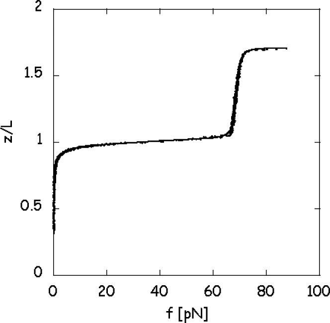
Figure 8: Least-squares fit of the Ising-DPC model to an overstretching dataset (48.5 kbp $\lambda$ DNA construct; buffer 500 mM NaCl, 20 mM Tris, pH 8). Data kindly supplied by C. Bustamante and S. Smith. Fit parameters: $\kappa^{{\mathrm{DPC}}}=\frac{3{k_{\rm B}}T}{2}\frac{1}{43.75\thinspace{\rm nm}},\bar{\alpha}=5.45\,,\beta=0.16\,,{\cal Q}=0.13\,,\zeta=1.76\,,E^{B}=1.2\cdot 10^{3}\,\mathrm{pN}$ and $E^{S}=1.0\cdot 10^{4}\,\mathrm{pN}$. $\chi^{2}=9.22$ at $N=825$, points with $1.11<\langle\frac{z}{L}\rangle<1.55$ were excluded from the fit. For further discussion see Sect. IV.4.

So far, we have not included stretch moduli for the B- and S-DNA. This is easily implemented to first order in $f/E$ by replacing $f$ with $f(1+\frac{f}{2E^{S,B}})$ in the matrix elements for the two states respectively (Eq. IV.2). This procedure yields theoretical force-extension curves like the ones plotted in Figs. (8) and (9).

In summary, our model contains the following seven parameters. $2\bar{\alpha}{k_{\rm B}}T$ is the free energy per unit length required to flip B-DNA into the $S$-state, and is measured in [J/nm]. ${\cal Q}$ measures the cooperativity of the transition and has units [1/nm]. $A$ is the bend stiffness parameter of B-DNA, with units [nm]. The dimensionless parameter $\beta$ is the ratio of the B- and S-DNA bend stiffnesses. $E^{B}$ and $E^{S}$ are the stretch stiffnesses of B and S-DNA, and are measured in pN. Finally, $\zeta$ is the dimensionless elongation factor associated with the B$\to$S transition.

IV.4 Discussion of fits

Our strategy is now as follows: first, we fit the part of the stretching curve well below 65 pN to a one-state, continuum model (i.e. to the EWLC), determining its effective spring constant and stretch modulus. The values thus obtained are used as initial guesses in a fit of the full curve to the Ising-DPC model. To improve convergence, we eliminate two of the parameters, as follows. First, we can get an accurate value for $E^{B}$ from the low force data, so we hold it fixed to this value during the full fit. Second, as described in Sect. III we can work out the low-force limit analytically, and from this obtain the effective spring constant $\kappa$ as a function of the model’s parameters. We invert this relation to get $A$ as a function of $\kappa$ and the other parameters. We substitute this $A$, holding $\kappa$ fixed to the value obtained by fitting the low-force data to an EWLC. We then fit the remaining five parameters ($\beta$, $\cal Q$, $\bar{\alpha}$, $E^{S}$ and $\zeta$) to the dataset.

The results of the fits obtained in this manner are collected in Figs. (8) and (9). Our Ising-DPC hybrid model fits the experimental data rather well, but with so many fit parameters one may ask whether the model actually makes any falsifiable predictions. To answer this question we note that the data below the transition suffice to fix $A$ and $E^{B}$ as usual, roughly speaking from the curvature and slope of the curve below the transition. Similarly, the data above the transition fix $A^{S}=\zeta\beta A$ and $E^{S}$. The vertical jump in the curve at the transition fixes $\zeta$. The horizontal location of the jump fixes $\bar{\alpha}$, and the steepness of the jump fixes the cooperativity ${\cal Q}$. Thus all of the model’s parameters are fixed by specific features of the data. Two additional, independent features of the data now remain, namely the rounding of the curve at the start and end of the transition. Our model predicts these features fairly succesfully.

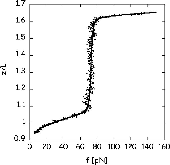
Figure 9: Least-squares fit of the Ising-DPC model to an overstretching dataset obtained from a 15.1 $\mu$m sample of EMBL3 $\lambda$ DNA in phosphate-buffered solution (100mM; 80mM Na⁺ and 0.01% Tween) from Cluzel et al. (1996). Data kindly supplied by J. Marko. Fit parameters: $\kappa^{{\mathrm{DPC}}}=\frac{3{k_{\rm B}}T}{2}\frac{1}{52.63\thinspace{\rm nm}},\bar{\alpha}_{0}=4.82\,\mathrm{nm}^{\raise 0.45206pt\hbox{${\scriptscriptstyle-}$}\kern-0.35002pt1}\,,\beta=0.08\,,{\cal Q}=0.23\,,\zeta=1.71\,,E^{B}=7.3\cdot 10^{2}\,\mathrm{pN}$ and $E^{S}=3\cdot 10^{4}\,\mathrm{pN}$. $\chi^{2}=2.15$ at $N=339$, points with $1.15<\langle\frac{z}{L}\rangle<1.5$ were excluded from the fit. For further discussion see Sect. IV.4.

Some common features emerging from the two fits deserve comment. First, both fits reproduce the known values for the effective persistence length of B-DNA of around $50\,$nm and its stretch modulus of about $1000\,$pN. Second, we can read off the bend stiffness of S-DNA from our fit as $A^{S}=\beta\zeta A=12.32\,$nm (data from Fig. 8) or 7.2 nm (data from Fig. 9). If S-DNA consisted of two unbound, single strands, we might have expected $A^{S}$ to be twice as large as the value $A^{\rm ss}\approx 0.85\,$nm obtained by fitting the single-strand stretching data with the continuum EDPC model (see Fig. 6). On the contrary, we find that the bend stiffness of S-DNA is intermediate between that of B-DNA and that of two single strands. This conclusion fits qualitatively with some of the structural models of S-DNA, in which the bases remain paired but are not stacked as in B-DNA.

Our third conclusion is that the stretch modulus of S-DNA is substantially higher than that of B-DNA. This conclusion is again consistent with the view of S-DNA as stabilized mainly by its backbones, which are much straighter than in B-DNA; the contour length of B-DNA is instead determined by weaker, base-stacking interactions.

IV.5 Relation to prior work

Polymer models with both finite cutoff and steric hindrances to motion are not new. Classical examples include the rotation-isomer models, in which succeeding monomers are joined by bonds of fixed polar angle but variable azimuthal angle Grosberg and Khlokhlov (1994). Models of this sort have had some success in making a priori predictions of the persistence length of a polymer from its structural information, but obtaining the force-extension relation is mathematically very difficult. Thus for example Miyake and Sakakibara (1962) obtain only the first subleading term in the low-force expansion. We are not aware of a prior formulation of a model incorporating the microscopic physics of discreteness and stiffness, with a detailed experimental test.

Several authors have also studied the entropic elasticity of two-state chains. As soon as the overstretching transition was discovered, Cluzel proposed a pure Ising model by analogy to the helix-coil transition Cluzel (1996). Others then introduced entropic elasticity, but required that both states have the same bending stiffness as B-DNA Marko (1998); Ahsan et al. (1998) or took one of the two states to be infinitely stiff Tamashiro and Pincus (2001), or to be a FJC Rouzina and Bloomfield (2001a, b). We believe our Ising-DPC model to be the first consistent formulation incorporating the coexistence of two different states with arbitrary elastic constants. Our approach also is calculationally more straightforward than some, and minimal in the sense that no unknown potential function needs to be chosen.

V Statistical analysis of the B$\to$S transition

Using standard techniques from statistical physics, we now look at the B$\to$S transition in some more detail. From the expressions for the Ising-DPC hybrid energy functional (25) and the partition function (26) we read off that the average “spin” $\sigma$ can be obtained as

$$\langle\sigma\rangle=\frac{1}{N}\frac{\partial}{\partial\alpha_{0}}\ln{\cal Z}=\frac{\partial}{\partial\bar{\alpha}}\Omega\,,$$ (46)

so that for instance the relative population of the S-state (or equivalently the probability to find an arbitrary segment in the S-state), $P(S)$, is given by

$$P(S)=\frac{1}{2}(1-\langle\sigma\rangle)\,.$$ (47)

Similarly, we can take the derivative of Eq. 26 with respect to $\gamma$ to determine the average nearest neighbor spin correlator

$$\langle\sigma_{i}\sigma_{i+1}\rangle=\frac{1}{N}\frac{\partial}{\partial\gamma}\ln{\cal Z}+1=1-2b{\cal Q}\frac{\partial}{\partial{\cal Q}}\Omega\,.$$ (48)

The quantity $\langle\sigma_{i}\sigma_{i+1}\rangle$ can be interpreted as the fraction of nearest neighbor pairs in the same state minus the fraction of pairs in opposite states. Consequently, the probability of having a spin flip at a given site is $P(\text{flip})=\tfrac{1}{2}(1-\langle\sigma_{i}\sigma_{i+1}\rangle)$ and the average number of S+B domain pairs is $N_{\mathrm{pairs}}=\tfrac{N}{2}P(\text{flip})$. A heuristic measure of the typical S-domain size is then Cantor and Schimmel (1980)

$$L_{\mathrm{dom}}=\frac{L}{N_{\rm pairs}}P(S)=\frac{2b(1-\langle\sigma\rangle)}{1-\langle\sigma_{i}\sigma_{i+1}\rangle}=\left(1-\frac{\partial\Omega}{\partial\bar{\alpha}}\right)/\left({\cal Q}\frac{\partial\Omega}{\partial{\cal Q}}\right)\,.$$ (49)

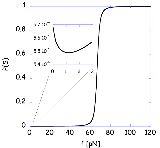
Figure 10: $P(S)$, the relative population of the S-state, versus the applied stretching force, as calculated from Eq. 47. The inset shows that the S-state has a nonzero population even at zero force. Parameter values are those from Fig. 9.

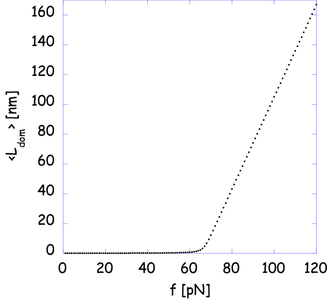
Figure 11: The typical length of an S-domain $L_{\mathrm{dom}}$ vs. the stretching force, calculated using Eq. 49. Parameter values are those of Fig. 9. The asymptotic slope of the linear increase has been determined to be $3.15$nm pN^-1. Note, that even at $120$pN, the typical size of an S-domain is only 160nm, or about 480 basepairs.

We wish to highlight two points from this discussion. First, Fig. 10 shows the fraction in the S-state, $P(S)$, as a function of the applied force, and we can see the characteristic sigmoidal behavior as the system is led through the transition. As the inset demonstrates, a small fraction is in the S-state even at zero force. This fraction initially decreases upon increasing the stretching force. Fig. 11 plots the typical S-domain length $L_{\rm dom}$ versus applied stretching force. It demonstrates how even well above the transition the S-state on average does not persist for very long; at the high end of the physically accessible range of forces S-domains measure about 160nm. This figure has some significance as it illustrates an important point about the role of nicks in the experiments. Empirically, when working with $\lambda$-phage DNA only around 5% of all samples are completely unnicked Léger (1999). Since the $\lambda$-phage genome is about 48Kbp in length, we can roughly estimate the probability for an arbitrary base pair to be unnicked is $P(\text{not})=(0.05)^{1/48000}$, and consequently the probability that a given pair is nicked is $P(\text{nick})=1-P(\text{not})\approx 6.2\cdot 10^{-5}$. Given the total length of $\lambda$-phage DNA, this implies we expect there to be an average of $6.2\cdot 10^{-5}\times 48\cdot 10^{3}\approx 3$ nicks per sample, corresponding to an average distance between nicks of the order of 5$\,\mu$m, considerably larger than the typical S-domain size. This observation bears on the question of the character of the S state of DNA Rouzina and Bloomfield (2001a): even if S-DNA were a denatured state, the existence of nicks would not necessarily cause it to suffer irreversible changes in its elasticity as tracts spanning two nicks fall off during overstretching.

Secondly, different groups have not agreed on whether the stretching curves of double-stranded and single-stranded DNA coincide at forces above the former’s overstretching transition Bustamante et al. (2000); Léger (1999). We wish to point out that even if S-DNA were a denatured state, we still would not necessarily expect these two curves to coincide. Fig. 10 shows that the conversion from B- to S-form continues well beyond the apparent end of the force plateau, continuing to affect the force-extension curve. To determine whether S-DNA is elastically similar to B-DNA one must disentangle the two states’ contributions to the stretching curve by globally fitting to a 2-state model, as we have done.

VI Conclusion

Sect. I summarizes our conclusions. Here we list a number of interesting modifications to the model, as possible extensions to this work.

While the variational approximation used here has proved to be adequate, still it is straightforward to replace it by the eigenfunction-expansion technique, which can be carried to arbitrary accuracy Marko and Siggia (1995). Similarly, the methods of Sect. III can be used to work in the full, discrete DPC model instead of the continuum approximation used in Sect. IV.3. It is also straightforward to retain finite-length effects, by keeping the subleading eigenvalue of the transfer matrix.

Real DNA is not a homogeneous rod. The methods of quenched disorder can be used to introduce sequence-dependent contributions to the transition free energy $\alpha$ and the bend stiffness $A$. Finally, we believe that the methods of this paper can be adapted to the study of the stretching of individual polypeptide and polysaccharide molecules Rief et al. (1998).

Appendix A Derivation of $y(\omega)$, the variational approximation to $\lambda_{\text{max}}$.

In this appendix we will derive an expression for $y(\omega)$ as defined in Eq. 18, which we recall reads

$$\|\vec{v}_{\omega}\|^{2}y(\omega)\equiv\vec{v}_{\omega}\cdot{\sf T}\cdot\vec{v}_{\omega}\,.$$ (50)

We will assume that the angles $\Theta_{i,i+1}$ between successive links are small, which allows us to replace $(\Theta_{i,i+1})^{2}=\arccos^{2}(\hat{t}_{i}\cdot\hat{t}_{i+1})$ by its small-angle approximation $2(1-\hat{t}_{i}\cdot\hat{t}_{i+1})$. The family of trial functions we use is parameterized by the single parameter $\omega$; $v_{\omega}(\hat{t}\,)\equiv e^{\omega\hat{t}\cdot\hat{z}}$. Furthermore, we will ignore the two contributions from the beginning and end of the chain (appearing for instance in Eq. 9), as they do not contribute to our result in the long chain limit anyway. Thus the energy functional is

$$\frac{{\cal E}[\{\hat{t}_{i}\}]}{{k_{\rm B}}T}=-\sum_{i=1}^{N-1}\left\{\frac{fb}{2{k_{\rm B}}T}\,(\hat{t}_{i}\cdot\hat{z}+\hat{t}_{i+1}\cdot\hat{z})\,-\frac{A}{b}(1-\hat{t}_{i}\cdot\hat{t}_{i+1})\right\}\,.$$ (51)

According to Eq. 13, the matrix elements of ${\sf T}$ are given by

$${\mathbb{T}}(\hat{t}_{i},\hat{t}_{i+1})=\exp\left[-\tilde{\ell}+\frac{\tilde{f}}{2}(\hat{t}_{i}+\hat{t}_{i+1})\cdot\hat{z}+\tilde{\ell}\,\hat{t}_{i}\cdot\hat{t}_{i+1}\right]\,,$$ (52)

where we use the dimensionless force $\tilde{f}\equiv\frac{fb}{{k_{\rm B}}T}$ and ratio of characteristic lengths $\tilde{\ell}=\frac{A}{b}$. Working out the scalar products in Eq. 50 yields

$$\|\vec{v}_{\omega}\|^{2}y(\omega)=e^{-\tilde{\ell}}\int_{{\mathbb{S}}^{2}}\!{\rm d}^{2}\hat{t}_{i}\int_{{\mathbb{S}}^{2}}\!{\rm d}^{2}\hat{t}_{i+1}\exp\left[(\frac{\tilde{f}}{2}+\omega)(\hat{t}_{i}+\hat{t}_{i+1})\cdot\hat{z}+\tilde{\ell}\,\hat{t}_{i}\cdot\hat{t}_{i+1}\right]\,.$$ (53)

Defining an auxiliary vector

$$\vec{G}\equiv(\frac{\tilde{f}}{2}+\omega)\hat{z}+\tilde{\ell}\,\hat{t}_{i}\equiv G\,\hat{g}\,,$$ (54)

with

$$G\equiv\|\vec{G}\|=\left((\frac{\tilde{f}}{2}+\omega)^{2}+\tilde{\ell}^{2}+\tilde{\ell}(\tilde{f}+2\omega)\,\hat{t}_{i}\cdot\hat{z}\right)^{\frac{1}{2}}\,,$$ (55)

simplifies Eq. 53, which now reads

$$\|\vec{v}_{\omega}\|^{2}y(\omega)=e^{-\tilde{\ell}}\int_{{\mathbb{S}}^{2}}\!{\rm d}^{2}\hat{t}_{i}\exp\left[(\frac{\tilde{f}}{2}+\omega)\hat{t}_{i}\cdot\hat{z}\right]\int_{{\mathbb{S}}^{2}}\!{\rm d}^{2}\hat{t}_{i+1}\exp\left[G\,\hat{g}\cdot\hat{t}_{i+1}\right]\,.$$ (56)

Transforming to spherical polar coordinates with $\hat{g}$ as the polar axis, the second integral can be worked out to give $\frac{4\pi}{G}\sinh(G)$. Since the integral over $\hat{t}_{i}$ involves only terms containing $\hat{t}_{i}\cdot\hat{z}$, the integration over the azimuthal angle simply yields $2\pi$. For the polar angle, we change the integration variable to $G$ (which is a monotonic function of $\hat{t}_{i}\cdot\hat{z}$), bringing it to the following form

$$\|\vec{v}_{\omega}\|^{2}y(\omega)=\frac{16\pi^{2}}{\tilde{\ell}(\tilde{f}+2\omega)}\exp\left[-\frac{3}{2}\tilde{\ell}-\frac{1}{2\tilde{\ell}}\left(\frac{\tilde{f}}{2}+\omega\right)^{2}\right]\int_{|\tilde{\ell}-(\frac{\tilde{f}}{2}+\omega)|}^{\tilde{\ell}+(\frac{\tilde{f}}{2}+\omega)}\!{\rm d}G\,\exp\left[G^{2}/2\tilde{\ell}\right]\sinh(G)\,.$$ (57)

The integral over $G$ can be performed analytically, and is most conveniently expressed in terms of error functions as

$$\int_{|\tilde{\ell}-(\frac{\tilde{f}}{2}+\omega)|}^{\tilde{\ell}+(\frac{\tilde{f}}{2}+\omega)}\!{\rm d}G\,\exp\left[G^{2}/2\tilde{\ell}\right]\sinh(G) =$$ (58)

$$\frac{e^{-\tilde{\ell}/2}\sqrt{-\pi\tilde{\ell}}}{2\sqrt{2}}\left[\text{Erf}\left(\frac{i}{2\sqrt{2\tilde{\ell}}}(\tilde{f}+4\tilde{\ell}+2\omega)\right)-\text{Erf}\left(\frac{i}{2\sqrt{2\tilde{\ell}}}(\tilde{f}-4\tilde{\ell}+2\omega)\right)\right]\,.$$

This expression is valid only in the regime where $\tilde{\ell}>\frac{\tilde{f}}{2}+\omega$, which is satisfied as long as one chooses $A>b$. Note that the error functions have imaginary arguments. Using the normalization quoted in Eq. 17 we can now express $y(\omega)$ in a form that is well suited for further (numerical) manipulations:

$$y(\omega) = \frac{2\sqrt{2}\pi^{3/2}\omega e^{-2\tilde{\ell}-\frac{(2\omega+\tilde{f})^{2}}{8\tilde{\ell}}}\text{csch}(2\omega)}{\sqrt{-\tilde{\ell}}(2\omega+\tilde{f})}\times$$ (59)

$$\times\left[\text{Erf}\left(\frac{i}{2\sqrt{2\tilde{\ell}}}(\tilde{f}+4\tilde{\ell}+2\omega)\right)-\text{Erf}\left(\frac{i}{2\sqrt{2\tilde{\ell}}}(\tilde{f}-4\tilde{\ell}+2\omega)\right)\right]\,.$$

References

- Ahsan et al. (1998) Ahsan, A., J. Rudnick, and R. Bruinsma, 1998. Elasticity theory of the B-DNA to S-DNA transition. Biophysical Journal 74, 132.
- Bouchiat et al. (1999) Bouchiat, C., M. D. Wang, J.-F. Allemand, T. Strick, S. M. Block, and V. Croquette, 1999. Estimating the persistence length of a worm-like chain molecule from force-extension measurements. Biophysical Journal 76, 409.
- Bustamante et al. (1994) Bustamante, C., J. Marko, E. D. Siggia, and S. Smith, 1994. Entropic elasticity of lambda-phage DNA. Science 265, 1599.
- Bustamante et al. (2000) Bustamante, C., S. B. Smith, J. Liphardt, and D. Smith, 2000. Single-molecule studies of DNA mechanics. Curr. Op. Str. Biol. 10, 279.
- Cantor and Schimmel (1980) Cantor, C. R., and P. R. Schimmel, 1980, Biophysical chemistry (W. H. Freeman, New York, NY), chapter 20.
- Clausen-Schaumann et al. (2000) Clausen-Schaumann, H., M. Rief, C. Tolksdorf, and H. E. Gaub, 2000. Mechanical stability of single DNA molecules. Biophysical Journal 78, 1997.
- Cluzel (1996) Cluzel, P., 1996, L’ADN, une molécule extensible, Ph.D. thesis, Université Paris VI, Paris.
- Cluzel et al. (1996) Cluzel, P., A. Lebrun, C. Heller, R. Lavery, J.-L. Viovy, D. Chatenay, and F. Caron, 1996. DNA: An extensible molecule. Science 271, 792.
- Flory (1969) Flory, P. J., 1969, Statistical Mechanics of Chain Molecules (Interscience, New York).
- Grosberg and Khlokhlov (1994) Grosberg, A. Y., and A. R. Khlokhlov, 1994, Statistical Physics of Macromolecules (American Institute of Physics Press, New York).
- Hegner et al. (1999) Hegner, M., S. B. Smith, and C. Bustamante, 1999. Polymerization and mechanical properties of single RecA-DNA filaments. Proc. Natl. Acad. Sci. USA 96, 10109.
- Kramers and Wannier (1941) Kramers, H. A., and G. H. Wannier, 1941. Statistics of the two-dimensional ferromagnet. Parts I&II. Phys. Rev. 60, 252.
- Kratky and Porod (1949) Kratky, O., and G. Porod, 1949. Röntgenuntersuchung gelöster Fadenmoleküle. Rec. Trav. Chim. Pays-Bas 68, 1106.
- Léger (1999) Léger, J.-F., 1999, L’ADN : une flexibilité structurale adaptée aux interactions avec les autres macromolécules de son environnement, Ph.D. thesis, Université Louis Pasteur, Strasbourg.
- Léger et al. (1999) Léger, J.-F., G. Romano, A. Sarkar, J. Robert, L. Bourdieu, D. Chatenay, and J. F. Marko, 1999. Structural transitions of a twisted and stretched DNA molecule. Phys. Rev. Lett. 83, 1066.
- Marko (1998) Marko, J., 1998. DNA under high tension: overstretching, undertwisting, and relaxation dynamics. Phys. Rev. E. 57, 2134.
- Marko and Siggia (1995) Marko, J. F., and E. D. Siggia, 1995. Stretching DNA. Macromolecules 28, 8759.
- Miyake and Sakakibara (1962) Miyake, A., and M. Sakakibara, 1962. Effect of hindering potential on the stretched chain configuration. J. Phys. Soc. Japan 17, 164.
- Rief et al. (1999) Rief, M., H. Clausen-Schaumann, and H. E. Gaub, 1999. Sequence-dependent mechanics of single DNA molecules. Nature Struct. Biol. 6, 346.
- Rief et al. (1998) Rief, M., P. Schulz-Vanheyden, and H. E. Gaub, 1998, in Nanoscale science and technology, edited by N. Garcia, M. Nieto-Vesperinas, and H. Rohrer (Kluwer, Dordrecht, NL), pp. 41–47.
- Rouzina and Bloomfield (2001a) Rouzina, I., and V. A. Bloomfield, 2001a. Force-induced melting of the DNA double helix 1. thermodynamic analysis. Biophysical Journal 80, 882.
- Rouzina and Bloomfield (2001b) Rouzina, I., and V. A. Bloomfield, 2001b. Force-induced melting of the DNA double helix 2. effect of solution contributions. Biophysical Journal 80, 894.
- Saito et al. (1967) Saito, N., K. Takahashi, and Y. Yunoki, 1967. The statistical mechanical theory of stiff chains. J. Phys. Soc. Japan 22, 219.
- Smith et al. (1996) Smith, S. B., Y. Cui, and C. Bustamante, 1996. Overstretching B-DNA: The elastic response of individual double-stranded DNA molecules. Science 271, 795.
- Tamashiro and Pincus (2001) Tamashiro, M. N., and P. Pincus, 2001. Helix–coil transition in homopolypeptides under stretching. Phys. Rev. E 63, 021909 (8 pages).
- Wang et al. (1997) Wang, M., H. Yin, R. Landick, J. Gelles, and S. Block, 1997. Stretching DNA with optical tweezers. Biophysical Journal 72, 1335.
- Yamakawa (1971) Yamakawa, H., 1971, Modern theory of polymer solutions (Harper and Row, New York).
- Zimm and Bragg (1959) Zimm, B. H., and J. K. Bragg, 1959. Theory of the phase transition between helix and random coil in polypeptide chains. J. Chem. Phys. 31, 526.