Metamorphosis of plasma turbulence–shear flow dynamics through a transcritical bifurcation

Abstract

The structural properties of an economical model for a confined plasma turbulence governor are investigated through bifurcation and stability analyses. A close relationship is demonstrated between the underlying bifurcation framework of the model and typical behavior associated with low- to high-confinement transitions such as shear flow stabilization of turbulence and oscillatory collective action. In particular, the analysis evinces two types of discontinuous transition that are qualitatively distinct. One involves classical hysteresis, governed by viscous dissipation. The other is intrinsically oscillatory and non-hysteretic, and thus provides a model for the so-called dithering transitions that are frequently observed. This metamorphosis, or transformation, of the system dynamics is an important late side-effect of symmetry-breaking, which manifests as an unusual non-symmetric transcritical bifurcation induced by a significant shear flow drive.

I

Fusion plasmas, and possibly other quasi two-dimensional fluid systems, may undergo a more-or-less dramatic transition from a low to a high confinement state (the L–H transition) as the power input is increased, with the desirable outcome that particle and energy confinement is greatly improved due to localized transport reduction Terry (2000). In this work we report on a bifurcation and stability probe of an economical model for L–H transition dynamics that uncovers a mechanism by which a radical change, or metamorphosis, may occur in the qualitative nature of the dynamics. We apply the results of this analysis to clarify the relationship between the structure of the model and the physics of the process that it describes, and draw comparisons with characteristics of L–H transitions observed in various experiments.

Since 1988 there has been much progress in developing low-dimensional (low-order or reduced) descriptions of L–H transition dynamics and associated oscillatory phenomena (see, for example, Refs Itoh and Itoh, 1988; Hinton, 1991; Diamond et al., 1994; Pogutse et al., 1994; Vojtsekhovich et al., 1995; Sugama and Horton, 1995; Lebedev et al., 1995; Drake et al., 1996; Hu and Horton, 1997; Takayama et al., 1998; Itoh et al., 1998; Staebler, 1999; Thyagaraja et al., 1999; Ball and Dewar, 2001), the driving force being the potential power of a unified, low-dimensional model as a predictive tool for the design and control of confinement states. For example, a model that speaks of the shape and extent of hysteresis in the L–H transition would help engineers who are interested in controlling access to H-mode. Given the many variables and parameters that could be varied around a hysteretic régime, it would be cheaper—i.e., save hundreds of cpu hours and/ or many expensive diagnostics—to know in advance which ones actually do affect the hysteresis, and which do not.

To help construe the context in which low-dimensional descriptions of plasma dynamics are sought, it is appropriate at this stage to make some general remarks. It makes sense to try to find the simplest description of an evolving system that is consistent with the time and space scales on which one is interested in making experimental observations of that system. One would like the description to incorporate the qualitative nature of the system structure and dynamics, so that it can be used for design and control purposes and make useful predictions. A truly useful description usually turns out to be a low-dimensional system of coupled ordinary differential equations. Such descriptions are powerful because they are supported by well-developed theories that give qualitative and global insight, such as bifurcation, stability, and symmetry theory Golubitsky and Schaeffer (1985); Holmes et al. (1996). In principle we can map analytically the bifurcation structure of the entire state and parameter space of a low-dimensional dynamical system, but this is not yet possible for an infinite-dimensional system.

However, the quest for a low-dimensional state space that captures the qualitative dynamics of L–H transitions has been problematic. It has been shown Ball and Dewar (2000, 2001) that some of the models cited above do not reflect salient features of L–H transitions such as shear flow suppression of turbulence, or are incomplete, or show profound structural discrepancies, although it is intuitively reasonable to expect that manifestly different models should be equivalent at some deeper level if they describe the same phenomena.

By economical, or minimal, model we mean the smallest, functionally simplest, and mathematically consistent model that captures qualitatively the dynamical traits that are typically observed over many experiments in different machines. The strength and potency of a minimal model is just this universality; its apparent disregard for details, numbers and unit dimensions is sometimes perceived—wrongly—as a weakness. In keeping with this ideology we introduce here a consensus dynamical model that is economical in terms of variables and parameters, and incorporates the smallest number of rate processes of simplest functional form needed to reflect the universally observed dynamics. If the model is successful we expect additional terms to have only quantitative, not qualitative or structural, effects. We should also be able to identify easily its limits of validity, or where it breaks down and why.

In section II we introduce the plasma turbulence governor as a useful schema to conceptualize and represent the major contributing rate and feedback processes, relating these to the corresponding dynamical system. Bifurcation and stability analyses and interpretive discussions, with reference to reported experiments, are given in the remaining sections. In section III we begin by determining the two highest order (most degenerate) singularities in the system, or organizing centers. Section IV describes the generic bifurcation diagram and discusses the hysteresis and limit cycles in the system. In section V we illustrate and discuss the useful properties of the two-parameter bifurcation diagram. This discussion leads in to section VI, in which we determine explicitly the transcritical metamorphosis to an oscillatory, non-hysteretic régime. A short summary is given in section VII. The Appendix contains a derivation of the dynamical equations.

II

The schematic in Fig. 1 is a primitive of a plasma turbulence governor. (The name is intended to refer to archetypical mechanical exemplars of feedback controllers such as James Watt’s 1788 steam-engine governor. In James (1987) a comparable scheme was called the “barotropic governor”, in the context of quasi two-dimensional atmospheric flows.)

Figure 1: Coupled rates and feedback processes that contribute to the dynamics of L–H transitions. Solid arrows indicate generation rates, wavy arrows dissipation, dashed arrows feedback on rate coefficients; black diamond indicates negative feedback.

A power input $q$ creates a pressure gradient $P$ from which the turbulent density fluctuation intensity $N$ grows at a rate with coefficient $\gamma$. The turbulence feeds energy into the poloidal shear flow $v$ via the Reynolds stress $\alpha$. The shear flow is generated externally at rate $\varphi$ and damped by the ion viscosity $\mu$. The turbulence is damped quadratically with coefficient $\beta$. Also indicated is a competitive distribution of energy from the pressure gradient, whereby different fractions may partition into turbulence generation and shear flow damping. It is not difficult to appreciate how the various rate and competitive processes in Fig. 1 could balance out—or rather, un-balance out—so as to give rise to the oscillatory and hysteretic dynamics that are characteristic of L–H transitions.

The reduced dynamical system that models this scheme is based on the Sugama-Horton model Sugama and Horton (1995), which itself was derived from approximate resistive MHD vorticity and pressure convection equations Strauss (1977, 1980):

$$\varepsilon\frac{dP}{dt}= q-\gamma PN$$ (1)

$$\frac{dN}{dt}= \gamma PN-\alpha v^{2}N-\beta N^{2}$$ (2)

$$2\frac{dv}{dt}= \alpha vN-\mu(P,N)v+\varphi$$ (3)

$$\mu(P,N)=bP^{m}+aP^{r}N.$$ (4)

In terms of the shear flow kinetic energy $F=v^{2}$ Eqs 2 and 3 may be written as

$$\frac{dN}{dt}= \gamma PN-\alpha FN-\beta N^{2}$$ (2^′)

$$\frac{dF}{dt}= \alpha FN-\mu(P,N)F+\varphi F^{1/2}.$$ (3^′)

The derivation of this system is given in the Appendix. The most important modification to the original Sugama-Horton model is the symmetry-breaking term $\varphi$ in Eq. 3. It will be seen that this term, which may be interpreted as an external shear flow driving rate, has dramatic effects on the bifurcation structure of the system.

The first and second terms in the bipartite viscosity function, Eq. 4, model the neoclassical and anomalous viscosity damping respectively. In a plasma of low collisionality the exponent $m$ is negative so a high pressure gradient has the effect of blocking the neoclassical contribution. (Refer to Fig. 1.) Under these circumstances energy can accumulate in the shear flow then feed back into turbulence decorrelation. On the other hand, a high pressure gradient and high turbulence levels both enhance the anomalous viscosity damping, because the exponent $r$ is positive. The net effect will depend on the relativity of the three competitive rates involved in the distribution of energy from the pressure gradient.

III

Generally in bifurcation analysis we are interested in the multiplicity, stability, singularity, and parameter dependence of zero solutions of a bifurcation equation $g=G(x,\lambda_{1},\lambda_{2},\ldots,\lambda_{n})$, where $x$ is a state variable and the $\lambda_{i}$ are parameters, that is derivable (in principle if not always in practice) from the equilibria of a dynamical system.

In Eqs 1–4 we may select $x\equiv P$ and the principal bifurcation parameter $\lambda_{1}\equiv q$ and set the right hand sides to zero to obtain the bifurcation equation,

$$g=\frac{1}{2P^{2}\alpha\gamma^{2}}\left(aP^{r}q-q\alpha+bP^{1+m}\gamma\right)\left(q\beta-P^{2}\gamma^{2}\right)+\frac{\varphi\left(P^{2}\gamma^{2}-q\beta\right)^{1/2}}{2\left(P\alpha\gamma\right)^{1/2}}$$ (5)

(where Eq. 3^′ has been used). Singular points occur where $g=g_{P}=0$. (Subscripts on $g$ denote partial derivatives with respect to the subscripted variable.) On the $v=0$ branch they are given by

$$(P,q,\varphi)=\left(P_{i},P_{i}^{2}\gamma^{2}/\beta,0\right),$$

with the $P_{i}$ given by the real, positive roots of $\beta b+P^{1-m}(aP^{r}-\alpha)\gamma=0$. At these points $g_{q}=0$ and $g_{PP}=-8\left(aP_{i}^{r}\left(-1-m+r\right)+\left(1+m\right)\alpha\right)\gamma^{2}/\left(\alpha\beta\right).$ Thus for some values of the exponents $m$ and $r$ one or more of the singularities may comply with the pitchfork conditions

$$g=g_{P}=g_{q}=0=g_{PP}=0,\,g_{PPP}\neq 0,\,g_{Pq}\neq 0.$$ (6)

Obviously (since $g_{PP}$ must equal 0), compliance with these conditions also implies the existence of hysteresis.

To specify the dependence of the viscosity damping on the pressure gradient in Eq. 4 we set $m=-3/2$ and $r=1$, as in Sugama and Horton (1995). This value of $m$ applies for the temperature dependence of the ion viscosity in a low collisional régime Braginskii (1965). The value of $r=1$ is the simplest that is consistent with the suggested dependence of the anomalous viscosity on the ion temperature in Sugama and Horton (1994a).

With this specification the conditions in Eq. 6 applied to Eq. 5 find the unique pitchfork P* as

$$\left(v,q,b,\varphi\right)=\left(0,\frac{\alpha^{2}\gamma^{2}}{9a^{2}\beta},\frac{2\alpha^{3}\gamma\sqrt{\alpha/a}}{27\sqrt{3}\>a^{2}\beta},0\right).$$ (P*)

At P* the two non-degeneracy conditions in Eq. 6 evaluate as $g_{Pq}=8a/\alpha$, $g_{PPP}=-18a\gamma^{2}/(\alpha\beta)$. A pitchfork is described as a codimension 2 singularity, because its universal unfolding requires 2 parameters additional to the principal bifurcation parameter. Note that the second unfolding parameter, chosen here as $b$, can be any of the dissipative parameters $a$, $b$, or $\beta$. For reference the bifurcation diagram in Fig. 2 has been computed and plotted for the critical set (P*). The singular point on the $v=0$ branch at high $q$ complies with the conditions

$$g=g_{P}=g_{q}=0,\,g_{PP}\neq 0,\,\det d^{2}g<0,$$ (7)

where $d^{2}g$ is the Hessian matrix of second partial derivatives $\left(\begin{array}[]{cc}\!g_{PP}&\!g_{qP}\\ g_{qP}&g_{qq}\end{array}\!\right).$ A singular point that satisfies these conditions is usually termed a transcritical bifurcation, or sometimes a “simple bifurcation”.

Figure 2: Bifurcation diagram for the critical set (P*), $\varphi=0$, $b=18.58$, $\alpha=2.4$, $\beta=1$, $\gamma=1$, $a=0.3$, $\varepsilon=1.5$.

For non-critical values of $b$ (i.e., $b\neq b_{\left({\text{P}}^{*}\right)}=18.58\ldots$), P* collapses to a second transcritical bifurcation on the $v=0$ branch. These two transcriticals coalesce and annihilate each other at a second codimension 2 singularity D* on the $v=0$ branch, defined by the conditions

$$g=g_{P}=g_{q}=\det d^{2}g=0,\,g_{PP}\neq 0,\,g_{Pq}\neq 0,$$ (8)

and found using Eq. 5 as

$$(v,q,b,\varphi)=\left(0,\frac{\left(5\alpha\gamma\right)^{2}}{\left(7a\right)^{2}\beta},\frac{50\sqrt{5\alpha/\left(7a\right)}\,\alpha^{3}\gamma}{7^{3}a^{2}\beta},0\right),$$ (D*)

with $g_{PP}=-32\gamma^{2}/\left(7\beta\right)$, $g_{Pq}=16a/(5\alpha)$. The bifurcation diagram showing this point (at $(v,q,b,\varphi)=(0,0.61\ldots,53.52\ldots,0)$ for values of the other parameters as in Fig. 2) would be extremely dull and flat—it consists only of the line $v=0$. Such a highly dissipative system has no interesting behaviour at all.

IV

A bifurcation diagram for non-critical values of the unfolding parameters $b$ and $\varphi$ is shown in Fig. 3. (In the bifurcation diagrams stable solution branches are indicated by solid lines, unstable branches by dashed lines, and the dotted lines trace out the maximum and minimum amplitude of limit cycle branches.) The symmetry evident in Fig. 2 is broken by selection of a small positive value of $\varphi$, which determines a preferred direction of the poloidal shear flow.

Figure 3: Bifurcation diagram with $b=1$, $\varphi=0.02$, other parameters as for Fig. 2.

Branches of stable limit cycles emanate from Hopf bifurcations on the $+v$ and $-v$ H-mode branches. They reflect reports from experiments that a transition to a quiescent H-mode can be achieved followed by the onset of oscillatory behaviour, or edge-localised modes (ELMs), as the power input continues to be increased Ida et al. (1990); Thomas et al. (1998); Igitkhanov et al. (1998); Shats (1999). The original Sugama-Horton model was found to exhibit a chaotic time series for a particular set of parameter values in this régime Bak et al. (2001). In our model we have found that this branch of limit cycles can undergo several successive period doublings followed by period halvings back to a period-one limit cycle.

The limit cycles are also extinguished at Hopf bifurcations. In Ball and Dewar (2001) it was shown that oscillatory behaviour is regulated by the contribution of the pressure gradient evolution. At moderately high power input the pressure gradient and turbulence are high, neoclassical viscous damping is inhibited, and large amplitude oscillations would be expected as energy alternately accumulates in the shear flow and is exchanged with the turbulence. The relative phases of $v$, $N$, and $P$ are shown in the time series of Fig. 4.

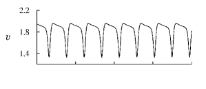
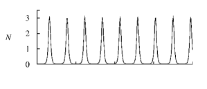
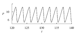
Figure 4: A time series for $q=4$ on the $+v$ branch. Other parameters are the same as in Fig. 3.

However, this is balanced by the enhancement of anomalous viscosity damping by the larger amounts of turbulence and pressure gradient energy at higher power inputs. (Refer to the governor schematized in Fig. 1.) As this anomalous viscosity effect begins to take over the amplitude of the limit cycles decreases rapidly until they are extinguished at the Hopf bifurcations at higher $q$.

Although definitive experiments have not yet been performed that measure the growth and extent of the H-mode oscillations over the power input, it is physically reasonable that they would be limited by some damping factor. The passage through an oscillatory régime with increasing power is a characteristic of type III ELMs Connor (1998); Suttrop (2000). However, the quantitative features of type III ELMs, such as the frequency spectrum, are not reproduced by this simple model.

On the $v<0$ branch the limit cycles are smaller in amplitude and occur over a smaller range of the power input. At $q\approx 2.5$, for example, the $+v$ H-mode is oscillatory but the $-v$ H-mode is quiescent. Again, to our knowledge the appropriate experiments have not yet been carried out, but this is reminiscent of the prescription given in ref. Burrell et al. (2001): “The key factors in creating the quiescent H-mode operation are neutral beam injection in the direction opposite to the plasma current (counterinjection) plus cryopumping to reduce the density.”

Reports of reversals in the direction of main or impurity ion poloidal shear flow Bell et al. (1998); Solomon (2001) can also be rationalized on the basis of Fig. 3. In a system that is evolved initially onto the $v<0$ branch, the poloidal shear flow must reverse if a perturbation decreases the power input slightly below that at the lower limit point. Shear flow reversal may also occur anywhere along the $v<0$ branch, if the system is given a sufficiently strong transient kick.

Note that in Fig. 3 the shear flow $v$ reaches a broad maximum with increasing power input, then decreases to the the pre-transition level given by the shear flow source. This would be reasonable behaviour on physical grounds—one would not expect the shear flow to increase indefinitely with power input, because the turbulent viscosity damping (the second term in Eq. 4 with $r=1$) begins to take over as the power input increases the pressure gradient.

Clearly there is scope for tuning other parameters in the model so as to obtain a complete picture of the steady states and limit cycles over parameter space, and more quantitative agreements with experiments. One may wish, for example, to maximize the range of $q$ over which turbulence stabilization occurs, or minimize the range of $q$ over which limit cycles occur, or both.

Figure 3 also shows the hysteresis that is predicted by compliance with the conditions in Eq. 6. Transitions with hysteresis have been observed in several machines: DIII-D Thomas et al. (1998), Asdex Upgrade Zohm et al. (1995); Ryter et al. (1998), JET, and in simulations of ITER Igitkhanov et al. (1998), and Alcator C-Mod Hubbard et al. (1998). Hysteresis is typically modified by dissipation, characterised in this model by the parameters $\beta$, $b$, and $a$. However, hysteresis does not seem to be a necessary or universal feature of discontinuous transitions.

One of the typical features of L–H transitions that a minimal model should reflect is suppression of the turbulence by the shear flow. Figure 5 shows the bifurcation diagram with the mean square turbulence level $N$ as the state variable, where for clarity only the curve that matches the positive $v$ branch is given. The turbulence is clearly suppressed over the hysteretic region, then begins to grow again as the higher pressure gradient from higher power input creates more turbulence.

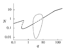
Figure 5: Bifurcation diagram with $N$ as chosen state variable, showing the curve that corresponds to the positive $v$ branch in Fig. 3.

V

The width and extent of hysteresis for selected values of $b$ can be judged from the two-parameter bifurcation diagram for the $+v$ branch in Fig. 6, in which computed curves of the singular points in Fig. 3 are shown. The solid lines mark the loci of limit points (which are also sometimes called fold or saddle-node bifurcations) as $b$ is varied. The dot-dash line is the locus of Hopf bifurcations as $b$ is varied.

Figure 6: Two-parameter curves of the singular points in Fig. 3. Solid lines are the loci of the limit points, dot-dash lines are the Hopf bifurcation loci.

If one can imagine taking slices across this diagram at various important values of $b$, the bifurcation story of the system can be told compactly, by inferring a reconstruction of the single-parameter $(q,v)$ bifurcation diagram corresponding to each selected value of $b$.

A slice taken above the critical value of $b$ at the cusp would yield a $(q,v)$ bifurcation diagram that shows no multiplicity of states. Thus, in a highly dissipative system any transition is expected to be smooth and gradual rather than discontinuous, and a number of experiments suggest this conjecture. In ASDEX Upgrade the power hysteresis disappears at higher density (which implies more collisional damping) where gradual rather than discontinuous confinement improvement occurs Ryter et al. (1998). A régime in which density fluctuation amplitudes are reduced continuously was also observed in Moyer et al. (1999). In Dahi et al. (1998) a discontinuous bifurcation of the electric field in a stellarator was reported for conditions of low neutral density, where the charge-exchange damping rate is low. The change in the electric field became gradual for conditions of high neutral density, because the charge-exchange damping rate increases. (The electric field is related to the poloidal shear flow and the pressure gradient through the radial force balance Shats et al. (1997).)

Oscillatory behaviour is also expected to be damped out at high dissipation rates. The maximum in the locus of Hopf bifurcations in Fig. 6 occurs at the value of $b$ where the two Hopf bifurcations on the $+v$ branch in Fig. 3 annihilate each other (or conversely, are created). Above this value of $b$ the $+v$ branch is stable with no associated limit cycles.

As slices are taken at lower $b$ the hysteresis and the range of oscillatory behavior evidently become broader. At low dissipation rates the feedback is strong and nonlinear behavior is expected to be more pronounced.

The crossing of the Hopf and limit point loci in Fig. 6 is non-local, i.e., the value of $P$ (and of $v$ and $N$) at the crossing on the Hopf curve is different from that on the limit point curve. Within the overlapping region a direct transition to an oscillatory H-mode may occur.

VI

The minimum in the limit point curve of Fig. 6 implies the existence of another transcritical bifurcation (defined by Eq. 7) in the system, that occurs at non-zero $v$. This non-symmetric transcritical bifurcation may have important issues concerning access to and control of confinement states. Consider the series of stills in Fig. 7, which snapshot $+v$ bifurcation diagram sections for increasing values of $\varphi$.

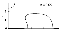
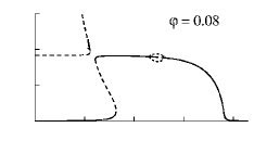
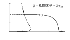
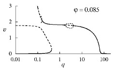
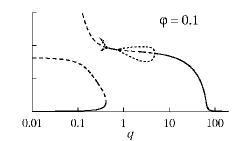
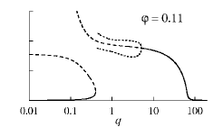
Figure 7: A series of bifurcation diagram snapshots taken at increasing values of $\varphi$ illustrates the exchange at $\varphi_{T_{m}}$ and its aftermath. Here $\varepsilon=1.0$ and other parameters are the same as in Fig. 3.

As $\varphi$ is incremented a separate branch of solutions to Eq. 5, which is trapped at $(q,v)=(0,\infty)$ for $\varphi=0$, begins to intrude more prominently into the physical region ($\varphi=0.05$). Although it is unstable at first, and therefore physically irrelevant for very small values of $\varphi$, it does not remain so. The singular occurrence of a zero real eigenvalue and a pair of complex conjugate eigenvalues with zero real part signals the appearance of a degenerate Hopf bifurcation. (Eigenvalues were computed numerically.)

Further increments in $\varphi$ separate the limit point and the Hopf bifurcation, between which the solutions are stable ($\varphi=0.08$). The branch of limit cycles that emanates from the Hopf bifurcation undergoes one or more period doubling bifurcations before ending, presumably at a homoclinic (infinite period) terminus. This branch of limit cycles is quite short, and thus not very well resolved in Fig. 7 for the lower values of $\varphi$. Note also that the branch of limit cycles emanating from the hysteretic solution branch has also appeared by $\varphi=0.08$.

At a metamorphic value of $\varphi$ that we designate $\varphi_{T}{{}_{m}}$ the arms of the two separate steady-state branches are exchanged at a transcritical bifurcation. We know this point is present because the defining conditions Eq. 7 are satisfied with $\varphi\neq 0$. (In numbers $(v,q,\varphi)_{T}{{}_{m}}=(1.8247..,0.1468..,0.08059..)$, with $\det d^{2}g=-0.004687..$, $g_{PP}=-0.001250..$, for values of the other parameters as given in Fig 3. Note that the value of $\varepsilon$ is irrelevant for calculating steady-state bifurcations such as the pitchfork and transcritical but not for Hopf bifurcations.)

After the exchange, e.g. at $\varphi=0.085$ and $\varphi=0.1$, we see the unusual occurrence of three Hopf bifurcations on the same branch, although this situation could be inferred from the shallow but distinct minimum and the maximum in the locus of Hopf bifurcations in Fig. 6.

The last frame of Fig. 7, for $\varphi=0.11$, is taken after the “new” and the lower-$q$ “old” Hopf bifurcations have collided and annihilated each other at a singular point associated with two zero eigenvalues. This is what the minimum in the curve of Hopf bifurcations means. The branch of limit cycles emanating from the upper-$q$ “old” Hopf bifurcation now continues to the (presumed) homoclinic terminus. There are a couple of period-doublings on it (not shown). We also see that the limit cycles are extinguished and a quiescent H-mode is achieved at the single remaining Hopf bifurcation.

Turning our attention to the stable part of the lower branch in the last frame of Fig. 7, we see that as $q$ is tuned past the lower limit point the system must jump to another stable attractor. This transition is very different from the intrinsically hysteretic transition depicted in Fig 3. Here the stable attractor on the upper branch is a limit cycle rather than a fixed point. Furthermore, this transition is not hysteretic. In fact, hysteresis is (locally) forbidden by the condition $g_{PP}\neq 0$ of Eq. 7. Therefore it is not modulated by dissipation in the same way as the transition in Fig.3, although the feedback itself is still due to nonlinear dissipation rates.

As the value of $\varphi$ is increased even further, bifurcation diagrams that one could plot gradually become less meaningful. This is because $\varphi=$ constant is a first approximation, valid for small $\varphi$, to to a nonlinear function $\varphi(\zeta)$, where $\zeta$ may include dynamical variables and parameters.

This type of transition could serve as a model for the dithering or L–H–L transitions, followed by a quiescent H-mode, that have been reported in many machines. Although there may be other mechanisms for dithering transitions—another possible scenario is given at the end of section V and indicated in Fig. 6, where an oscillatory transition may occur in a very poorly dissipative system—we have at least a preliminary semiological and classification guide: if your transition is oscillatory and non-hysteretic then perhaps you should look for a strong shear flow source, if it is strongly hysteretic perhaps you should look at dissipation mechanisms. Some experimental evidence supports the idea that dithering transitions result from a strong shear flow source. In Hugill et al. (1998), an analysis of time series data around the L–H transition in COMPASS-D suggested that a homoclinic orbit is involved in the change of stability at the transition. In stellarator W7-AS typically the quiescent ELM-free H-mode is obtained after a phase characterized by quasi-periodic ELMs Hirsch et al. (1998, 2000). In H1 stellarator a transition to fluctuating H-mode occurs at lower gas filling pressures and lower magnetic fields than the transition to quiescent H-mode Shats and Rudakov (1997).

In terms of the governor in Fig. 1 a shear flow that is generated internally and driven externally at comparable rates is likely to give rise to interesting non-linear dynamics, because more kinetic energy in the shear flow leads to more turbulence suppression through decorrelation, but also a larger damping effect, which then alters the competitive distribution of energy from the pressure gradient.

VII

In summary, this reduced dynamical model, comprised simply of energy input, exchange, and loss rates, reflects generic characteristics of confined plasma bulk dynamics that have not been reflected in previous models. The bifurcation and stability analysis also reveals two qualitatively different transitions. The hysteretic transition is controlled by the damping rate coefficients. The non-hysteretic transition occurs when there is a relatively strong shear flow drive.

Symmetry-breaking in this system has two major effects. Firstly, a non-zero shear flow drive is physically inevitable, even in the best-controlled experiments, and it determines a preferred direction for the shear flow. Secondly, it interacts with the internal generation and loss dynamics to cause the metamorphosis shown in Fig. 7.

More generally, the information obtained from this analysis strengthens the thesis developed in Holmes et al. (1996): that remarkably low-dimensional models can capture and help explain essential aspects of turbulent flows that elude understanding from numerical simulations that include resolved spatial scales, and that physical deductions can be made from observations of bifurcations.

Appendix

Reduced MHD fluid equations in tokamak and stellarator geometries were originally derived by Strauss Strauss (1977, 1980). In the electrostatic approximation, a damped MHD fluid may be described by the following momentum and pressure convection equations:

$$\rho\frac{d{\rm\mathbf{v}}}{dt} =-\nabla p+{\rm\mathbf{J}}\times{\rm\mathbf{B}}+\mu\nabla_{\perp}^{2}{\rm\mathbf{v}}+\Omega^{\prime}\tilde{p}\hat{x}-\rho\nu\left({\rm\mathbf{v}}-V\left(x\right)\hat{y}\right)$$ (9)

$$\frac{dp}{dt} =\chi\nabla_{\perp}^{2}p,$$ (10)

where $d/dt=\partial/\partial t+{\rm\mathbf{v}}\cdot\nabla$, together with the incompressibility condition $\nabla\cdot{\rm\mathbf{v}}=0$ and the resistive Ohm’s law ${\rm\mathbf{E}}+{\rm\mathbf{v}}\times{\rm\mathbf{B}}=\eta{\rm\mathbf{J}}$. The symbols and notation are explained in table 1. The curl of Eq. 9 yields a vorticity equation, which is sometimes preferred in two-dimensional fluid dynamics, but we have used the momentum form because it is more transparent physically and has a simpler correspondence to the kinetic energy. An infinite slab configuration is used for simplicity and generality, as was also assumed in Stix (1973) for a drift-kinetic treatment of plasma relaxation. It is sketched in Fig. 8, where the region $-\delta<x<\delta$ can be taken to represent a region at the edge or within a confined plasma where a transport barrier evolves.

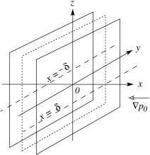
Figure 8: Simple slab geometry is assumed. The plasma edge region is $-\delta<x<\delta$, with $x=\delta$ at the plasma surface. $\nabla p_{0}<0$ is the $y,z$-averaged pressure gradient.

The last term on the right hand side of Eq. 9 removes the nonlinear shear-flow reversal symmetry of the system under $v_{x}(x,y,t)\rightarrow v_{x}(x,-y,t)$, $v_{y}(x,y,t)\rightarrow-v_{y}(x,-y,t)$, $\tilde{p}(x,y,t)\rightarrow\tilde{p}(x,-y,t)$, $V(x)\rightarrow V(x)$. Similar equations, without the symmetry-breaking term in the momentum balance, have been used by several authors Carreras et al. (1987); Sugama and Wakatani (1988); Sugama and Horton (1994a, b, 1995) as a basis for studying resistive turbulence–flow interactions. The symmetry-breaking term was introduced in Sugama and Horton (1994a), but only a posteriori as an adjunct in an equation for the background poloidal flow. Here we introduce it at the outset. It models the friction force acting between the single-fluid plasma velocity $\mathbf{v}$ and an assumed external poloidal flow $V\hat{y}$. Although $V\hat{y}$ may be described for convenience as an external velocity, the term represents any asymmetric shear-inducing mechanism, such as friction with neutrals, non-ambipolar ion orbit losses, or neoclassical effects not included in the slab model.

The symmetry operation on $v_{0}(x)\equiv\langle v_{y}\rangle(x)$ and $V(x)$ is sketched in Fig. 9. We are working in the frame in which there is no electrostatic potential difference across the slab. That is, it is assumed that we have made a Galilean transformation to the frame in which the spatial average of $v_{0}$ across the slab is zero. For simplicity we also assume that the spatial average of $V$ is zero.

Figure 9: Without the friction force the system is invariant under the transformation $v_{0}(x,t)\rightarrow-v_{0}(x,t)$ (solid line), $V(x)\rightarrow V(x)$ (dashed line). When the friction coefficient $\nu\neq 0$ the symmetry is broken.

Equations 9 and 10 are not intended to express a detailed fluid description of a plasma, but are intended instead to represent a qualitatively authentic, semi-empirical model for the essential generation and loss processes that give rise to the turbulence–shear flow interactions that we have schematized in Fig. 1 as the plasma turbulence governor. The dynamical system Eqs 1–3 can be derived from Eqs 9 and 10, following the spatial averaging procedure implicit in Sugama and Horton (1995).

First of all, the dynamics of the mean flow $v_{0}=\langle v_{y}\rangle$ are extracted from the first moment ($v_{y}\hat{y}$) of $\langle$ Eq. 9 $\rangle$ as

$$\partial_{t}v_{0}-\mu\partial^{2}_{x}v_{0}+\partial_{x}\langle\tilde{v}_{x}\tilde{v}_{y}\rangle=-\nu(v_{0}-V),$$ (11)

the energy moment of which gives the spatially averaged evolution of shear flow kinetic energy $F$:

$$\begin{split}\frac{d}{dt}\left[\frac{1}{\delta}\int_{-\delta}^{\delta}\frac{dx}{2}\>v_{0}^{2}\right]&=-\frac{1}{\delta}\int_{-\delta}^{\delta}dx\>\left[\mu\left(\frac{dv_{0}}{dx}\right)^{2}+\nu\>v_{0}^{2}\right]\\ &\quad\quad+\frac{1}{\delta}\int_{-\delta}^{\delta}dx\>\langle\tilde{v}_{x}\tilde{v}_{y}\rangle\frac{dv_{0}}{dx}\\ &\quad\quad\quad\quad+\frac{1}{\delta}\int_{-\delta}^{\delta}dx\>\nu Vv_{0}.\end{split}$$ (12)

This may be written as

$$\frac{dF}{dt}=-\epsilon_{F}+E_{F}+E_{\varphi},$$ (13)

where the definitions of $\epsilon_{F}$, $E_{F}$, and $E_{\varphi}$ correspond respectively to each term on the right hand side of Eq. 12 and $F\equiv\frac{1}{\delta}\int_{-\delta}^{\delta}\frac{dx}{2}\>v_{0}^{2}$.

Next, the second moment of Eq. 9 gives the total rate of evolution of $F$ and turbulent kinetic energy $N$:

$$\begin{split}\frac{d}{dt}\left[\frac{1}{\delta}\int_{-\delta}^{\delta}\frac{dx}{2}\left(v_{0}^{2}+\tilde{v}^{2}\right)\right]&=\frac{1}{\delta}\int_{-\delta}^{\delta}dx\>\Omega^{\prime}\frac{\left<\tilde{p}\,\tilde{v}_{x}\right>}{\rho}\\ &\quad-\frac{1}{\delta}\int_{-\delta}^{\delta}dx\,\left[\frac{\eta}{\rho_{m}}\left<\tilde{J}_{\parallel}^{2}\right>+\mu\left<\left(\frac{\partial\tilde{v}_{i}}{\partial x_{j}}\right)^{2}\right>\right]\\ &\quad\quad-\frac{1}{\delta}\int_{-\delta}^{\delta}dx\>\left[\mu\left(\frac{dv_{0}}{dx}\right)^{2}+\nu\>v_{0}^{2}\right]\\ &\quad\quad\quad+\frac{1}{\delta}\int_{-\delta}^{\delta}dx\>\nu Vv_{0},\end{split}$$ (14)

which may be expressed succinctly as

$$\frac{d}{dt}\left[F+N\right]=E_{N}-\epsilon_{N}-\epsilon_{F}+E_{\varphi}$$ (15)

where $E_{N}$ and $\epsilon_{N}$ are defined by the first two terms on the right hand side of Eq. 14 and $N\equiv\frac{1}{\delta}\int_{-\delta}^{\delta}\frac{dx}{2}\>\tilde{v}^{2}$ .

Finally, the evolution of potential energy in the pressure gradient is defined from the $x$-moment of Eq. 10, assuming the cross-field thermal transport $\chi\nabla_{\perp}^{2}$ can be neglected:

$$\frac{d}{dt}\left[\frac{1}{\delta}\int_{-\delta}^{\delta}dx\>\left(-x\right)\Omega^{\prime}\frac{p_{0}}{\rho}\right]=\frac{\langle\tilde{p}\tilde{v}_{x}\rangle|_{-\delta}^{\delta}}{\rho}\Omega^{\prime}-\frac{1}{\delta}\int_{-\delta}^{\delta}dx\>\frac{\langle\tilde{p}\tilde{v}_{x}\rangle}{\rho}\Omega^{\prime},$$ (16)

or

$$\frac{dP}{dt}=E_{P}-E_{N},$$ (17)

with the input rate $E_{P}$ defined as the first term on the right hand side and $P\equiv\frac{1}{\delta}\int_{-\delta}^{\delta}dx\>\left(-x\right)\Omega^{\prime}p_{0}/\rho$.

The spatially averaged dynamical system thus consists of Eqs 15, 13, and 17. For closure we follow Sugama and Horton (1995), using the approximations $p_{0}(x)\simeq p_{0}(x=\delta)+xdp_{0}/dx$ and $v_{0}(x)\simeq v_{0}(x=\delta)+xdv_{0}/dx$ for the background pressure and flow profiles and re-defining $P$ and $F$ as the gradient terms alone. Approximations or expressions based on empirical arguments were given in Sugama and Horton (1995) for the rates in Eqs 13, 15, and 17. The rates given in Eqs 1–3 are economized versions of those expressions, in the sense that simpler power laws were chosen if this did not result in any qualitative changes to the singularity and stability structure of the system. The rationale is that for most of the rates we shall only learn from experiments whether different powers apply, meanwhile simple power laws give more transparent algebra. We approximate the energy transfer rate from the pressure gradient simply as $E_{N}\simeq(\gamma/\varepsilon)PN$, and the energy transfer rate between the turbulence and the shear flow, due to the Reynolds stress, as $E_{F}\simeq\alpha FN$. The power input through the boundary is defined as $E_{p}\equiv q/\varepsilon$. The two-timing coefficient $\varepsilon$ is related to the thermal capacitance, and regulates the contribution of the pressure gradient to the dynamics. For the dissipative terms we take the turbulent energy dissipation rate as $\epsilon_{N}\simeq\beta N^{2}$ and the shear flow energy damping rate as $\epsilon_{F}\simeq\mu(P,N)F$, assuming the viscous damping to be dominant in $\epsilon_{F}$. The external shear flow driving rate is then $E_{\varphi}\simeq\varphi F^{1/2}$, with $\varphi\simeq\delta\nu V$. To obtain the evolution of the shear flow in terms of a velocity gradient variable we re-define $v\equiv\pm F^{1/2}$. Eqs 1–3 ensue.

$\mathbf{v}=\frac{1}{B_{0}}\mathbf{\hat{z}}\times\nabla\phi=\mathbf{v}_{0}+\tilde{\mathbf{v}}$	$\mathbf{E}\times\mathbf{B}$ flow velocity
$\mathbf{v}_{0}=\langle\mathbf{v}\rangle$	average background component
$\tilde{\rm\mathbf{v}}$	fluctuating or turbulent component
$p=p_{0}+\tilde{p}$	plasma pressure
$p_{0}=\langle p\rangle$	average background component
$\tilde{p}$	fluctuating or turbulent component
$\rho$	average mass density of ions, assumed constant
$\mu$	ion viscosity coefficient
$B_{0}$	magnetic field along the $z$ axis
$\eta$	resistivity
$\nu$	frictional damping coefficient
$\Omega^{\prime}\equiv d\Omega/dx>0$	average field line curvature, assumed constant
$\nabla_{\perp}^{2}$	$\partial^{2}_{x}+\partial^{2}_{y}$
$\nabla_{\parallel}$	$\partial_{z}+\frac{x}{L_{s}}\partial_{y}$
$\chi$	cross-field thermal transport coefficient
$V$	external flow
$\langle\cdots\rangle$	average on $(y,z)$ plane

Table 1: Glossary of symbols, terms, and notation.