Faddeev-Merkuriev equations for resonances in three-body Coulombic systems

Abstract

We reconsider the homogeneous Faddeev-Merkuriev integral equations for three-body Coulombic systems with attractive Coulomb interactions and point out that the resonant solutions are contaminated with spurious resonances. The spurious solutions are related to the splitting of the attractive Coulomb potential into short- and long-range parts, which is inherent in the approach, but arbitrary to some extent. By varying the parameters of the splitting the spurious solutions can easily be ruled out. We solve the integral equations by using the Coulomb-Sturmian separable expansion approach. This solution method provides an exact description of the threshold phenomena. We have found several new $S$-wave resonances in the $e^{-}e^{+}e^{-}$ system in the vicinity of thresholds.

1 Introduction

Certainly, to calculate resonances in three body atomic systems the methods based on complex coordinates are the most popular. The complex rotation of the coordinates turns the resonant behavior of the wave function into a bound-state-like asymptotic behavior. Then, standard bound-state methods become applicable also for calculating resonances. The complex rotation of the coordinates does not change the discrete spectrum, the branch cut, corresponding to scattering states, however, is rotated down onto the complex energy plane, and as a consequence, resonant states from the unphysical sheet become accessible.

In practice bound state variational approaches are used, that results in a discretization of the rotated continuum. By changing the rotation angle the points corresponding to the continuum move, while those corresponding to discrete states, like bound and resonant states, stay. This way one can determine resonance parameters.

However, in practical calculations the points of the discretized continuum scatter around the rotated-down straight line. So, especially around thresholds it is not easy to decide whether a point is a resonance point or it belongs to the rotated continuum.

Recently, we have developed a method for calculating resonances in three-body Coulombic systems by solving homogeneous Faddeev-Merkuriev integral equations [1] using the Coulomb-Sturmian separable expansion approach [2]. As a test case, we calculated the resonances of the negative positronium ion. We found all the $12$ resonances presented in Ref. [3] and observed good agreements in all cases.

With our method we succeeded in locating $10$ more resonances in the same energy region, all of them are very close to the thresholds. This is certainly due to the fact that in Ref. [2] the threshold behaviors are exactly taken into account. Unexpectedly we also observed that in the case of attractive Coulomb interactions the Faddeev-Merkuriev integral equations produce numerous resonant solutions of dubious origin. We tend to regard them as spurious resonances which come about from the somewhat arbitrary splitting of the potential in the three-body configuration space into short-range and long-range terms, that is an inherent attribute of the theory.

Since the possible appearance of spurious states in the formalism is new and surprising, for the sake of the better understanding of its mechanism, in Section 2 we outline briefly the Faddeev-Merkuriev integral equation formalism. In our particular case of the $e^{-}e^{+}e^{-}$ system two particles are identical and the set of Faddeev-Merkuriev integral equations can be reduced to an one-component equation. In Section 3 we discuss the spurious solutions. In Section 4 the Coulomb-Sturmian separable expansion method is applied to the one-component integral equation. In Section 5 we present our new calculations for the $L=0$ resonances of the $e^{-}e^{+}e^{-}$ system and compare them with the results of the complex scaling calculations of Ref. [3].

2 Faddeev-Merkuriev integral equations

The Hamiltonian of a three-body Coulombic system is given by

$$H=H^{0}+v_{1}^{C}+v_{2}^{C}+v_{3}^{C},$$ (1)

where $H^{0}$ is the three-body kinetic energy operator and $v_{\alpha}^{C}$ denotes the Coulomb potential in the subsystem $\alpha$, with $\alpha=1,2,3$. We use throughout the usual configuration-space Jacobi coordinates $x_{\alpha}$ and $y_{\alpha}$. Thus $v_{\alpha}^{C}$, the potential between particles $\beta$ and $\gamma$, depends on $x_{\alpha}$.

The Hamiltonian (1) is defined in the three-body Hilbert space. The three-body kinetic energy, when the center-of-mass motion is separated, is given by

$$H^{0}=h^{0}_{x_{\alpha}}+h^{0}_{y_{\alpha}}=h^{0}_{x_{\beta}}+h^{0}_{y_{\beta}}=h^{0}_{x_{\gamma}}+h^{0}_{y_{\gamma}},$$ (2)

where $h^{0}$ is the two-body kinetic energy. The two-body potential operators are formally embedded in the three-body Hilbert space $v^{C}=v^{C}(x){\bf 1}_{y}$, where ${\bf 1}_{y}$ is a unit operator in the two-body Hilbert space associated with the $y$ coordinate.

Merkuriev proposed [1] to split the Coulomb interaction in the three-body configuration space into short- and long-range terms

$$v_{\alpha}^{C}=v_{\alpha}^{(s)}+v_{\alpha}^{(l)},$$ (3)

where the short- and long-range parts are defined via a splitting function:

$$v_{\alpha}^{(s)} = v_{\alpha}^{C}\zeta(x_{\alpha},y_{\alpha})$$ (4)

$$v_{\alpha}^{(l)} = v_{\alpha}^{C}\left[1-\zeta(x_{\alpha},y_{\alpha})\right].$$ (5)

The splitting function $\zeta$ is defined in such a way that

$$\lim_{x,y\to\infty}\zeta(x,y)=\left\{\begin{array}[]{ll}1,&\mbox{if}\ |x|<x^{0}(1+|y|/y^{0})^{1/\nu},\\ 0,&\mbox{otherwise,}\end{array}\right.$$ (6)

where $x^{0},y^{0}>0$ and $\nu>2$. Usually the functional form

$$\zeta(x,y)=2/\left\{1+\exp\left[{(x/x^{0})^{\nu}}/{(1+y/y^{0})}\right]\right\},$$ (7)

is used. So, the separation into short- and long-range parts is made along a parabola-like curve over the $\{x,y\}$ plane. Typical shapes for $v^{(s)}$ and $v^{(l)}$ are shown in Figures 1 and 2, respectively.

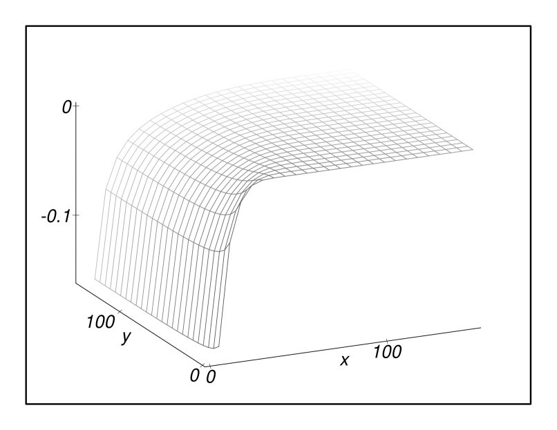
Figure 1: Typical shape of $v^{(s)}$ for attractive Coulomb potentials.

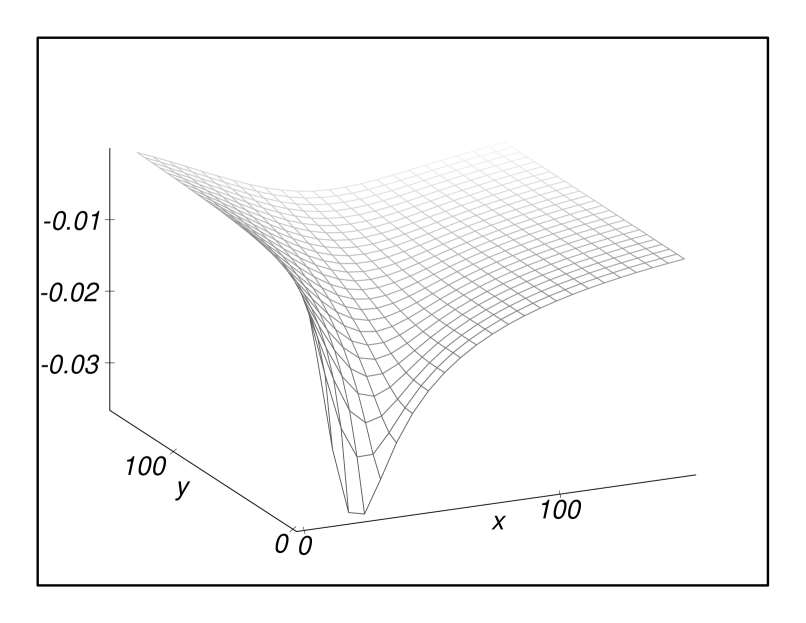
Figure 2: Typical shape of $v^{(l)}$ for attractive Coulomb potentials.

In atomic three-particle systems the sign of the charge of two particles are always identical. Let us denote in our $e^{-}e^{+}e^{-}$ system the two electrons by $1$ and $2$, and the positron by $3$. In this case $v_{3}^{C}$, the interaction between the two electrons, is a repulsive Coulomb potential which does not support two-body bound states. Therefore the entire $v_{3}^{C}$ can be considered as long-range potential. With splitting (3) the Hamiltonian can formally be written in a form which looks like an usual three-body Hamiltonian with two short-range potentials

$$H=H^{(l)}+v_{1}^{(s)}+v_{2}^{(s)},$$ (8)

where the long-range Hamiltonian is defined as

$$H^{(l)}=H^{0}+v_{1}^{(l)}+v_{2}^{(l)}+v_{3}^{C}.$$ (9)

Then, the Faddeev method is applicable and, in this particular case, results in a splitting of the wave function into two components

$$|\Psi\rangle=|\psi_{1}\rangle+|\psi_{2}\rangle,$$ (10)

with components defined by

$$|\psi_{\alpha}\rangle=G^{(l)}(z)v_{\alpha}^{(s)}|\Psi\rangle,$$ (11)

where $\alpha=1,2$ and $G^{(l)}(z)=(z-H^{(l)})^{-1}$, $z$ is a complex number.

In the case of bound and resonant states the wave-function components satisfy the homogeneous two-component Faddeev-Merkuriev integral equations

$$|\psi_{1}\rangle = G_{1}^{(l)}(z)v^{(s)}_{1}|\psi_{2}\rangle$$ (12)

$$|\psi_{2}\rangle = G_{2}^{(l)}(z)v^{(s)}_{2}|\psi_{1}\rangle$$ (13)

at real and complex energies, respectively. Here $G^{(l)}_{\alpha}$ is the resolvent of the channel long-ranged Hamiltonian $H^{(l)}_{\alpha}=H^{(l)}+v_{\alpha}^{(s)}$, $G^{(l)}_{\alpha}(z)=(z-H^{(l)}_{\alpha})^{-1}$. Merkuriev has proved that Eqs. (12-13) possess compact kernels, and this property remains valid also for complex energies $z=E-i\Gamma/2$, $\Gamma>0$.

Further simplification can be achieved if we take into account that the two electrons, particles $1$ and $2$, are identical and indistinguishable. Then, the Faddeev components $|\psi_{1}\rangle$ and $|\psi_{2}\rangle$, in their own natural Jacobi coordinates, have the same functional forms

$$\langle x_{1}y_{1}|\psi_{1}\rangle=\langle x_{2}y_{2}|\psi_{2}\rangle=\langle xy|\psi\rangle.$$ (14)

On the other hand

$$|\psi_{2}\rangle=p{\mathcal{P}}|\psi_{1}\rangle,$$ (15)

where ${\mathcal{P}}$ is the operator for the permutation of indexes $1$ and $2$ and $p=\pm 1$ are eigenvalues of ${\mathcal{P}}$. Therefore we can determine $|\psi\rangle$ from the first equation only

$$|\psi\rangle=G_{1}^{(l)}v_{1}^{(s)}p{\mathcal{P}}|\psi\rangle.$$ (16)

It should be emphasized, that so far we did not make any approximation, and although this integral equation has only one component, yet it gives full account both of asymptotic and symmetry properties of the system.

3 Spurious resonance solutions

Let us suppose for a moment that the $y^{0}$ parameter in $\zeta(x_{1},y_{1})$ is infinite. Then $\zeta$ would not depend on $y_{1}$, the separation of the potential into short and long range parts would go along a straight line, and $v_{1}^{(l)}(x_{1},y_{1})$ would be like a valley in the $y_{1}$ direction. The potential $v_{1}^{(l)}(x_{1},y_{1})$, which is Coulomb-like along $x_{1}$, would support infinitely many bound states and, as free motion along the coordinate $y_{1}$ would be possible, the Hamiltonian $H^{0}+v_{1}^{(l)}$ would have infinitely many two-body channels.

If, however, $y^{0}$ is finite, the straight line along the $y_{1}$ direction becomes a parabola-like curve and the valley, as $y_{1}$ goes to infinity, gets broader and broader and shallower and shallower, and finally disappears (see Fig 2). As the valley gets closed the continuum of $H^{0}+v_{1}^{(l)}$ associated with the $y_{1}$ coordinate becomes discretized. So, if $y^{0}$ is finite, $H^{0}+v_{1}^{(l)}$ have infinitely many bound states. Similar analysis is valid also for $H^{0}+v_{2}^{(l)}$, and consequently, also $H^{(l)}$ has infinitely many bound states.

This, however, due to (11), can lead to spurious solutions. If, at some energy, $H^{(l)}$ has bound state $G^{(l)}$ has pole. Then, $|\psi_{\alpha}\rangle$ in Eq.  (11), irrespective of $v^{(s)}_{\alpha}$, can be finite even if $|\Psi\rangle$ is infinitesimal. These solutions are called spurious solutions: although the Faddeev components are not identically zero, but their sum vanishes.

Let us examine now the spectral properties of the Hamiltonian

$$H_{1}^{(l)}=H^{(l)}+v^{(s)}_{1}=H^{0}+v_{1}^{C}+v_{2}^{(l)}+v_{3}^{C}.$$ (17)

The three-body potential $v_{2}^{(l)}$ is attractive and constructed so that $v_{2}^{(l)}(x_{2},y_{2})$ vanishes as $y_{2}$ tends to infinity. Therefore, there are no two-body channels associated with fragmentation $2$, and of course neither with fragmentation $3$, the Hamiltonian $H_{1}^{(l)}$ has only $1$-type two-body asymptotic channels.

What happens to the bound states associated with $v_{2}^{(l)}$? They are embedded in the the continuum of $H^{0}+v_{1}^{C}$, and become resonant states. So, by solving the Faddeev-Merkuriev integral equations, at some complex energies, we can encounter spurious solutions. These spurious solutions are not related to the Hamiltonian $H$, but rather only to some auxiliary potentials coming from the splitting procedure. Consequently, the spurious resonances should be sensitive to the parameters of $\zeta$, while the physical resonances not. This way we can easily distinguish between physical and spurious resonance solutions.

4 Coulomb-Sturmian potential separable expansion approach

We solve Eq. (16) by using the Coulomb–Sturmian separable expansion approach [4]. The Coulomb-Sturmian (CS) functions are defined by

$$\langle r|nl\rangle=\left[\frac{n!}{(n+2l+1)!}\right]^{1/2}(2br)^{l+1}\exp(-br)L_{n}^{2l+1}(2br),$$ (18)

with $n$ and $l$ being the radial and orbital angular momentum quantum numbers, respectively, and $b$ is the size parameter of the basis. The CS functions $\{|nl\rangle\}$ form a biorthonormal discrete basis in the radial two-body Hilbert space; the biorthogonal partner is defined by $\langle r|\widetilde{nl}\rangle=\langle r|{nl}\rangle/r$. Since the three-body Hilbert space is a direct product of two-body Hilbert spaces an appropriate basis can be defined as the angular momentum coupled direct product of the two-body bases

$$|n\nu l\lambda\rangle_{1}=|nl\rangle_{1}\otimes|\nu\lambda\rangle_{1},\ \ \ \ (n,\nu=0,1,2,\ldots),$$ (19)

where $|nl\rangle_{1}$ and $|\nu\lambda\rangle_{1}$ are associated with the coordinates $x_{1}$ and $y_{1}$, respectively. With this basis the completeness relation takes the form (with angular momentum summation implicitly included)

$${\bf 1}=\lim\limits_{N\to\infty}\sum_{n,\nu=0}^{N}|\widetilde{n\nu l\lambda}\rangle_{1}\;\mbox{}_{1}\langle{n\nu l\lambda}|=\lim\limits_{N\to\infty}{\bf 1}^{N}_{1}.$$ (20)

Note that similar bases can be constructed for fragmentations $2$ and $3$ as well.

We make the following approximation on Eq. (16)

$$|\psi\rangle=G_{1}^{(l)}{\bf 1}^{N}_{1}v_{1}^{(s)}p{\mathcal{P}}{\bf 1}^{N}_{1}|\psi\rangle,$$ (21)

i.e. the operator $v_{1}^{(s)}p{\mathcal{P}}$ in the three-body Hilbert space is approximated by a separable form, viz.

$$v_{1}^{(s)}p{\mathcal{P}} = \lim_{N\to\infty}{\bf 1}^{N}_{1}v_{1}^{(s)}p{\mathcal{P}}{\bf 1}^{N}_{1}$$ (22)

$$\approx {\bf 1}^{N}_{1}v_{1}^{(s)}p{\mathcal{P}}{\bf 1}^{N}_{1}\approx\sum_{n,\nu,n^{\prime},\nu^{\prime}=0}^{N}|\widetilde{n\nu l\lambda}\rangle_{1}\;\underline{v}_{1}^{(s)}\;\mbox{}_{1}\langle\widetilde{n^{\prime}\nu^{\prime}l^{\prime}\lambda^{\prime}}|,$$

where $\underline{v}_{1}^{(s)}=\mbox{}_{1}\langle n\nu l\lambda|v_{1}^{(s)}p{\mathcal{P}}|n^{\prime}\nu^{\prime}l^{\prime}\lambda^{\prime}\rangle_{1}$. The compactness of the equation and the completeness of the basis guarantee the convergence of the method. Utilizing the properties of the exchange operator ${\mathcal{P}}$ these matrix elements can be written in the form $\underline{v}_{1}^{(s)}=p\times(-)^{l^{\prime}}\;\mbox{}_{1}\langle n\nu l\lambda|v_{1}^{(s)}|n^{\prime}\nu^{\prime}l^{\prime}\lambda^{\prime}\rangle_{2}$.

With this approximation, the solution of Eq. (16) turns into solution of matrix equations for the component vector $\underline{\psi}=\mbox{}_{1}\langle\widetilde{n\nu l\lambda}|\psi\rangle$

$$\{[\underline{G}^{(l)}_{1}(z)]^{-1}-\underline{v}^{(s)}_{1}\}\underline{\psi}=0,$$ (23)

where $\underline{G}_{1}^{(l)}=\mbox{}_{1}\langle\widetilde{n\nu l\lambda}|G_{1}^{(l)}|\widetilde{n^{\prime}\nu^{\prime}l^{\prime}\lambda^{\prime}}\rangle_{1}$. A unique solution exists if and only if

$$D(z)\equiv\det\{[\underline{G}^{(l)}_{1}(z)]^{-1}-\underline{v}^{(s)}_{1}\}=0.$$ (24)

The Green’s operator $\underline{G}_{1}^{(l)}$ is related to the Hamiltonian $H_{1}^{(l)}$, which is still a three-body Coulomb Hamiltonian, seems to be as complicated as $H$ itself. However, $H_{1}^{(l)}$ has only $1$-type asymptotic channels, with asymptotic Hamiltonian

$$\widetilde{H}_{1}=H^{0}+v_{1}^{C}.$$ (25)

Therefore, in the spirit of the three-potential formalism [5], $\underline{G}_{1}^{(l)}$ can be linked to the matrix elements of $\widetilde{G}_{1}(z)=(z-\widetilde{H}_{1})^{-1}$ via solution of a Lippmann-Schwinger equation,

$$(\underline{G}^{(l)}_{1})^{-1}=(\underline{\widetilde{G}}_{1})^{-1}-\underline{U}_{1},$$ (26)

where ${\underline{\widetilde{G}}_{1}}=\mbox{}_{1}\langle\widetilde{n\nu l\lambda}|\widetilde{G}_{1}|\widetilde{n^{\prime}\nu^{\prime}l^{\prime}{\lambda}^{\prime}}\rangle_{1}$ and ${\underline{U}_{1}}=\mbox{}_{1}\langle n\nu l\lambda|(v_{2}^{(l)}+v_{3}^{C})|n^{\prime}\nu^{\prime}l^{\prime}{\lambda}^{\prime}\rangle_{1}$.

The most crucial point in this procedure is the calculation of the matrix elements $\underline{\widetilde{G}}_{1}$, since the potential matrix elements $\underline{v}^{(s)}_{1}$ and $\underline{U}_{1}$ can always be evaluated numerically by making use of the transformation of Jacobi coordinates [6]. The Green’s operator $\widetilde{G}_{1}$ is a resolvent of the sum of two commuting Hamiltonians, $\widetilde{H}_{1}=h_{x_{1}}+h_{y_{1}}$, where $h_{x_{1}}=h^{0}_{x_{1}}+v_{1}^{C}(x_{1})$ and $h_{y_{1}}=h^{0}_{y_{1}}$, which act in different two-body Hilbert spaces. Thus, $\widetilde{G}_{1}$ can be given by a convolution integral of two-body Green’s operators, i.e.

$$\widetilde{G}_{1}(z)=\frac{1}{2\pi{i}}\oint_{C}dz^{\prime}\,g_{x_{1}}(z-z^{\prime})\;g_{y_{1}}(z^{\prime}),$$ (27)

where $g_{x_{1}}(z)=(z-h_{x_{1}})^{-1}$ and $g_{y_{1}}(z)=(z-h_{y_{1}})^{-1}$. The contour $C$ should be taken counterclockwise around the continuous spectrum of $h_{y_{1}}$ such a way that $g_{x_{1}}$ is analytic on the domain encircled by $C$.

In time-independent scattering theory the Green’s operator has a branch-cut singularity at scattering energies. In our formalism $\widetilde{G}_{1}(E)$ should be understood as $\widetilde{G}_{1}(E)=\lim_{\varepsilon\to 0}\widetilde{G}_{1}(E+{\mathrm{i}}\varepsilon)$, with $\varepsilon>0$, and $E<0$, since in this work we are considering resonances below the three-body breakup threshold. To calculate resonant states $\widetilde{G}_{1}(E+{\mathrm{i}}\varepsilon)$ has to be continued analytically to negative $\varepsilon$ values. Before doing that let us examine $\widetilde{G}_{1}(E+{\mathrm{i}}\varepsilon)$ with $\varepsilon>0$. Now, the spectra of $g_{y_{1}}(z^{\prime})$ and $g_{x_{1}}(E+{\mathrm{i}}\varepsilon-z^{\prime})$ are well separated and the spectrum of $g_{y_{1}}$ can easily be encircled such that the spectrum of $g_{x_{1}}$ does not penetrate into the encircled area (Fig. 3). Next, the contour $C$ is deformed analytically in such a way that the upper part descends into the unphysical Riemann sheet of $g_{y_{1}}$, while the lower part of $C$ is detoured away from the cut (Fig. 4). The contour still encircles the branch cut singularity of $g_{y_{1}}$, but in the $\varepsilon\to 0$ limit it now avoids the singularities of $g_{x_{1}}$. Moreover, by continuing to negative values of $\varepsilon$, in order that we can calculate resonances, the pole singularities of $g_{x_{1}}$ move onto the second Riemann sheet of $g_{y_{1}}$ (Fig. 5). Thus, the mathematical conditions for the contour integral representation of $\widetilde{G}_{1}(z)$ in Eq. (27) can be fulfilled also for complex energies with negative imaginary parts. In this respect there is only a gradual difference between the bound- and resonant-state calculations. Now, the matrix elements $\underline{\widetilde{G}}_{\alpha}$ can be cast in the form

$$\widetilde{\underline{G}}_{1}(z)=\frac{1}{2\pi{i}}\oint_{C}dz^{\prime}\,\underline{g}_{x_{1}}(z-z^{\prime})\;\underline{g}_{y_{1}}(z^{\prime}),$$ (28)

where the corresponding CS matrix elements of the two-body Green’s operators in the integrand are known analytically for all complex energies (see [5] and references therein). It is also evident that all the thresholds, corresponding to the poles of $\underline{g}_{x_{1}}$, are at the right location and therefore this method is especially suited to study near-threshold resonances.

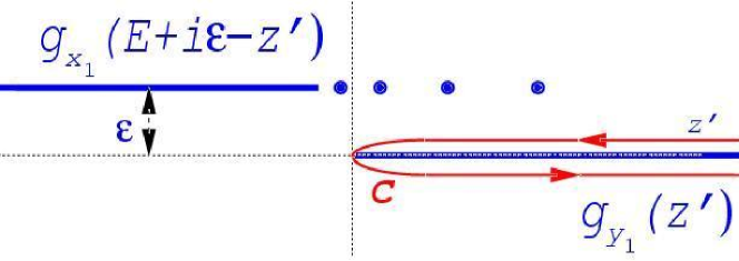
Figure 3: Analytic structure of $g_{x_{1}}(E+{\mathrm{i}}\varepsilon-z^{\prime})\;g_{y_{1}}(z^{\prime})$ as a function of $z^{\prime}$, $\varepsilon>0$. The Green’s operator $g_{y_{1}}(z^{\prime})$ has a branch-cut on the $[0,\infty)$ interval, while $g_{x_{1}}(E+{\mathrm{i}}\varepsilon-z^{\prime})$ has a branch-cut on the $(-\infty,E+{\mathrm{i}}\varepsilon]$ interval and infinitely many poles accumulated at $E+{\mathrm{i}}\varepsilon$ (denoted by dots). The contour $C$ encircles the branch-cut of $g_{y_{1}}$. In the $\varepsilon\to 0$ limit the singularities of $g_{x_{1}}(E+{\mathrm{i}}\varepsilon-z^{\prime})$ would penetrate into the area covered by $C$.

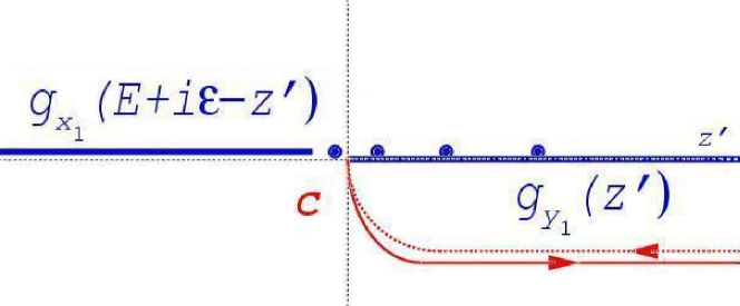
Figure 4: The contour of Fig. 3 is deformed analytically such that a part of it goes on the unphysical Riemann-sheet of $g_{y_{1}}$ (drawn by broken line) and the other part detoured away from the cut. Now, the contour avoids the singularities of $g_{x_{1}}(E+{\mathrm{i}}\varepsilon-z^{\prime})$ even in the $\varepsilon\to 0$ limit.

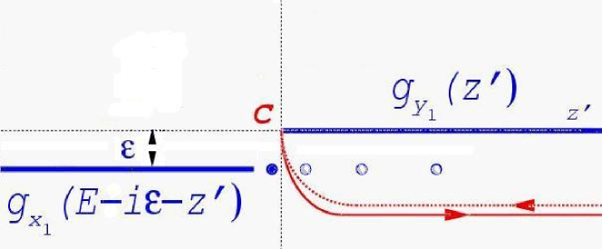
Figure 5: In the $\varepsilon<0$ case, what is needed to calculate resonances, the poles of $g_{x_{1}}$ which lie above the branch point of $g_{y_{1}}$ go to the unphysical sheet of $g_{y_{1}}$ (denoted by shaded points), while the others remain on the physical one.

5 $S$-wave resonances in positronium ion

To calculate resonances we have to find the complex zeros of the Fredholm determinant (24). To locate them we calculate $D(z)$ along the real energy axis with small step size. In the vicinity of zeros the $D(z)$ exhibits violent changes. Then we have a good starting point for the zero search. This way we can easily find resonances, at least the narrow ones. To find broad resonances one should proceed by calculating $D(E-i\varepsilon)$ with finite $\varepsilon>0$.

For the parameters of the splitting function we take $y^{0}=50\mbox{a}_{0}$ and $\nu=2.1$, $a_{0}$ is the Bohr radius. To select out the physical solutions we vary the short- and long-range potentials by taking $x^{0}=18\mbox{a}_{0},25\mbox{a}_{0}$ and $30\mbox{a}_{0}$, respectively. We can also vary the potentials by adding and subtracting a short-range term

$$v_{1}^{(s)} = v_{1}^{C}\zeta(x_{1},y_{1})+v_{0}\zeta(x_{1},y_{1})$$ (29)

$$v_{1}^{(l)} = v_{1}^{C}\left[1-\zeta(x_{1},y_{1})\right]-v_{0}\zeta(x_{1},y_{1}),$$ (30)

respectively, while keeping a fixed $x^{0}=18\mbox{a}_{0}$ value. This new kind of splitting goes beyond the Merkuriev’s original suggestion, but since the character of $v^{(s)}$ and $v^{(l)}$ remained the same all the nice properties of the original Faddeev-Merkuriev equations are retained. In these calculations we used $v_{0}=0,0.01,0.02$ values.

We found that some solutions, especially their widths, are very sensitive to the change of either $x^{0}$ or $v_{0}$ parameters. We regard them spurious solutions. Those solutions, given in Table I, were stable against all changes of parameters and we can consider them as physical resonances. We recovered all the resonances presented in Ref. [3] with very good agreements, but besides that we found $10$ more resonances, all of them are in the vicinity of some thresholds.

State	Ref. [3]		Our work
${}^{1}S^{e}$	$-E_{r}$	$\Gamma$	$-E_{r}$	$\Gamma$
	0.1520608	0.000086	0.15192	0.0000426
	0.12730	0.00002	0.12727	0.0000084
			0.1251	0.000002
	0.070683	0.00015	0.70666	0.000074
	0.05969	0.00011	0.059682	0.0000526
			0.0564	0.00003
	0.04045	0.00024	0.40426	0.0001294
	0.0350	0.0003	0.0350206	0.00013
	0.03463	0.00034	0.0346234	0.0001586
			0.03263	0.0001
			0.03158	0.00007
	0.0258	0.00045	0.02606	0.000104
	0.02343	0.00014	0.023428	0.0000436
${}^{3}S^{e}$	$-E_{r}$	$\Gamma$	$-E_{r}$	$\Gamma$
	0.12706	0.00001	0.127050	0.0000000028
			0.1251	0.000000001
	0.05873	0.00002	0.05872	0.0000001852
			0.0561	0.0000002
			0.0553	0.0001
	0.03415	0.00002	0.0342018	0.00000070
			0.03237	0.0000011
			0.03172	0.0000002
			0.031035	0.0000938

Table 1: $L=0$ resonances of $\mbox{Ps}^{-}$. The energies and widths are expressed in Rydbergs.

6 Conclusions

In this article we pointed out that in the Faddeev-Merkuriev integral equation approach of the three-body Coulomb problem the complex-energy spectrum is contaminated with spurious solutions. The spurious solutions, however, are sensitive to the splitting of the potential into short- and long-range terms. This offers an easy way to select the physical solutions.

We solved the integral equations by using the Coulomb-Sturmian separable expansion approach. This method gives an exact description of the threshold phenomena, thus the method is ideal for studying close-to-threshold resonances. In the $e^{-}e^{+}e^{-}$ system we located $10$ new resonances, all of them are in the close vicinity of some threshold.

This work has been supported by the NSF Grant No.Phy-0088936 and OTKA Grants under Contracts No. T026233 and No. T029003.

References

- [1] S. P. Merkuriev, Ann. Phys. (NY), 130, 395 (1980); L. D. Faddeev and S. P. Merkuriev, Quantum Scattering Theory for Several Particle Systems, (Kluver, Dordrech), (1993).
- [2] Z. Papp, J. Darai, C-.Y. Hu, Z. T. Hlousek, B. Kónya and S. L. Yakovlev, Phys. Rev. A 65, 032725 (2002).
- [3] Y. K. Ho, Phys. Lett., 102A, 348 (1984).
- [4] Z. Papp and W. Plessas, Phys. Rev. C, 54, 50 (1996).
- [5] Z. Papp, C-.Y. Hu, Z. T. Hlousek, B. Kónya and S. L. Yakovlev, Phys. Rev. A, 63, 062721 (2001).
- [6] R. Balian and E. Brézin, Nuovo Cim. B 2, 403 (1969).