TUNING KNOBS FOR THE NLC FINAL FOCUS 

Abstract

Compensation of optics errors at the Interaction Point (IP) is essential for maintaining maximum luminosity at the NLC. Several correction systems (knobs) using the Final Focus sextupoles have been designed to provide orthogonal compensation of linear and the second order optics aberrations at IP. Tuning effects of these knobs on the 250 GeV beam were verified using tracking simulations.

1 INTRODUCTION

The NLC Final Focus (FFS) optics [1] is designed to produce a very small vertical beam size of 3 nm at the Interaction Point (IP) in 500 GeV cms collisions. To attain these small spots, the NLC FFS design includes a number of non-linear elements; the optics for the NLC FFS is shown in Fig. 1, where sextupoles are denoted with first letter “S”, octupoles with “O”, and decapoles with “D”. These correctors are used to compensate the high-order geometric and chromatic effects generated in the nominal FFS optics as well as fold the beam halo in on itself to reduce the number of large amplitude halo particles [2].

Unfortunately, alignment and field errors in the FFS are amplified by the strong focusing and may lead to enlargement of IP beam size and subsequent luminosity loss. To maintain the maximum luminosity, aberrations increasing the beam size at IP have to be corrected. The correction procedure envisioned for the NLC FFS is very similar to that implemented on the Stanford Linear Collider (SLC) FFS or the Final Focus Test Beam (FFTB) [3]:

1. the quadrupoles are aligned using beam-based alignment techniques such as the shunting method,

2. the sextupoles are aligned in a similar manner,

3. trajectories are fit to verify the first-order optics and fix the phase advance between sextupoles,

4. the sextupoles are set to minimize the chromaticity,

5. global tuning correctors (knobs) are used to tune both the first-order and the nonlinear corrections using luminosity measurements.

In the following, we describe a set of simple correction system (knobs) using a minimum number of magnets for independent control of individual IP aberrations. The knob correctors are located at optimum optical positions close to the IP to minimize the extent of optics perturbation. Several knobs based on the FFS sextupoles have beed designed to correct linear and the second order optical aberrations at the IP.

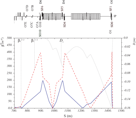
Figure 1: Optics and correctors in the NLC Final Focus.

2 LINEAR KNOBS

Five knobs have been designed to correct the following linear aberrations at the IP: longitudinal position of horizontal ($x$) and vertical ($y$) beta waist, $x$ and $y$ dispersion, and $x$-$y$ coupling. Correction of the first order aberrations requires adjustment of the normal and skew quadrupole field in the FFS. Similar to tuning techniques at the SLC [4] and the FFTB, we used $x$, $y$ offsets of the FFS sextupoles to make these knobs. One can verify that a sextupole displaced by $\Delta x$ and $\Delta y$ generates the following low order field on the reference orbit:

$$\Delta B_{y}=(-B^{\prime\prime}\Delta x)x+(B^{\prime\prime}\Delta y)y+B^{\prime\prime}\frac{\Delta x^{2}-\Delta y^{2}}{2},$$ (1)

$$\Delta B_{x}=(-B^{\prime\prime}\Delta x)y-(B^{\prime\prime}\Delta y)x+B^{\prime\prime}\Delta x\Delta y,\;\;\;\;\;\;\;\;\;\vspace{-3mm}$$ (2)

where $B^{\prime\prime}\!=\!\frac{\partial^{2}B_{y}}{\partial x^{2}}$ is the sextupole gradient. Therefore, the feed-down normal and skew quadrupole strengths are

$$\Delta K_{1n}=-K_{2}\Delta x,\;\;\;\;\;\Delta K_{1s}=K_{2}\Delta y,\vspace{-1mm}$$ (3)

respectively, where $K_{m}\!=\!\frac{1}{B\rho}\frac{\partial^{m}B_{y}}{\partial x^{m}}$ and $B\rho$ is the magnetic rigidity. The last terms in Eqn. 1, 2 lead to additional orbit, quadratic in $\Delta x$, $\Delta y$, which may be not negligible for large offsets, however, it is assumed that this orbit will be cancelled by the IP steering correctors. Correction efficiency of the FFS sextupoles is enhanced by the large beta functions and phase advance of $\Delta\mu^{s}\!=\!\pi/2\!+\!n\pi$ from IP.

2.1 Waist and Horizontal Dispersion

Enlargement of IP beam size and subsequent luminosity loss may be caused by longitudinal displacement $\Delta s$ of focusing waist and residual horizontal dispersion $\Delta\eta_{x}^{*}$ at IP. The waist displacement increases IP beta function as $\beta\!=\!\beta^{*}\!+\!\frac{\Delta s^{2}}{\beta^{*}}$, where $\beta^{*}$ is the ideal beta at IP. For maximum luminosity, waist position has to be kept within $\Delta s\!\ll\!\beta^{*}$.

The beta waist and horizontal dispersion knobs have been constructed using horizontal sextupole offsets. According to Eqn. 3, $\Delta x$ creates a normal quadrupole field which distorts $\beta_{x,y}$ and $\eta_{x}$ functions. Beta perturbation propagates to the IP and for $\Delta\mu^{s}\!=\!\pi/2\!+\!n\pi$ results in a longitudinal shift of the beta waist. The shift caused by a single sextupole is approximately

$$\Delta s_{x,y}\approx\pm K_{2}L\Delta x\,\beta_{x,y}^{s}\beta_{x,y}^{*}\cos{2\Delta\mu_{x,y}^{s}}\,,\vspace{-2mm}$$ (4)

where $L$ and $\beta^{s}$ are the sextupole length and beta function. As shown in Fig. 1, the dispersion $\eta_{x}^{s}$ is not zero in most of the FFS sextupoles, therefore $\Delta x$ also generates horizontal dispersion at IP:

$$\Delta\eta_{x}^{*}=K_{2}L\Delta x\,\eta_{x}^{s}\sqrt{\beta_{x}^{s}\beta_{x}^{*}}\sin{\Delta\mu_{x}^{s}}.\vspace{-2mm}$$ (5)

Three sextupoles are required to construct three orthogonal knobs for the $\Delta s_{x,y}$ and $\Delta\eta_{x}^{*}$ aberrations. In each knob, the sextupole offsets are varied linearly with the fixed scale factors to produce a desired amplitude of the aberration. The scale factors for $\Delta x$ offsets are listed in Table 1. Note that two sextupoles are sufficient for $\Delta s_{y}$ and $\Delta\eta_{x}^{*}$ knobs for the following reasons. In the first case, the ratio $\eta_{x}^{s}/\sqrt{\beta_{x}^{s}}$ at SD0 and SF1 is about constant which results in correction of $\Delta\eta_{x}^{*}$ when $\Delta s_{x}$ is corrected. In the second case, the $-I$ transformation between SF5 and SF6 makes it possible to cancel $\Delta s_{x}$ and $\Delta s_{y}$ with one scale factor.

Table 1: $\Delta x$ scale factors for $\Delta s_{x,y}$ and $\Delta\eta_{x}^{*}$ knobs.

Sextupole	SD0	SF1	SF5	SF6
$\Delta s_{x}$	1	0.6151	0	-6.1249
$\Delta s_{y}$	1	0.6151	0	0
$\Delta\eta_{x}^{*}$	0	0	1	0.2609

MAD [5] calculations show the following effects from these knobs: $\Delta s_{x}\!\approx\!-3122\,\Delta x_{{\scriptscriptstyle SD0}}$, $\Delta s_{y}\!\approx\!-60.36\,\Delta x_{{\scriptscriptstyle SD0}}$, $\Delta\eta_{x}^{*}\!\approx\!-0.4981\,\Delta x_{{\scriptscriptstyle SF5}}$. It is expected that $x$, $y$ resolution of sextupole movers will be close to 50 nm which is sufficient for accurate tuning of $\Delta s_{x,y}$ and $\Delta\eta_{x}^{*}$ – if desired, the magnet could be split onto two movers which would effectively reduce the required resolution.

2.2 Vertical Dispersion and Coupling

Orthogonal knobs to correct the vertical dispersion and betatron coupling at IP have been constructed using vertical sextupole offsets. The $\Delta y$ offsets create a skew quadrupole field which couples the $x$ and $y$ motion. Vertical dispersion at IP, caused by a single sextupole, is given by

$$\Delta\eta_{y}^{*}=-K_{2}L\Delta y\,\eta_{x}^{s}\sqrt{\beta_{y}^{s}\beta_{y}^{*}}\sin{\Delta\mu_{y}^{s}}.\vspace{-2mm}$$ (6)

In general, betatron coupling is described by four orthogonal matrix terms which can be independently tuned at IP using four skew quadrupoles located at the following phase advance from IP: $[\Delta\mu_{x},\Delta\mu_{y}]\!=\![0,0],[\frac{\pi}{2},0],[0,\frac{\pi}{2}],[\frac{\pi}{2},\frac{\pi}{2}]$. However, by design, all FFS sextupoles are located at $\Delta\mu_{x,y}^{s}\!=\!\pi/2\!+\!n\pi$ from IP, and hence only one coupling term can be created using the sextupoles. Regardless, this is the dominant coupling term in the FFS since most aberrations will be created by quadrupoles with the largest beta functions which are at the same phase as the sextupoles. The remaining three coupling terms can be compensated using three additional skew quadrupoles in the FFS system. So far, it has been found that the effect of the three minor terms is rather small and there is a full 4-D coupling correction section upstream of the beam delivery system.

Two sextupoles were used in the knobs for vertical dispersion and coupling as shown in Table 2, where the scale factors for $\Delta y$ are listed. The SD0, SD4 offsets cancel vertical dispersion and create coupling, while SF5 and SF6, located $-I$ apart, do the opposite. The effect of $\Delta\eta_{y}^{*}$ knob is estimated to be about $\Delta\eta_{y}^{*}\!\approx\!0.06918\,\Delta y_{{\scriptscriptstyle SF5}}$. This produces noticeable enlargement of vertical beam size when $\Delta y_{{\scriptscriptstyle SF5}}$ is a few microns. The beam sensitivity is much greater to the coupling knob, where an offset of $\Delta y_{{\scriptscriptstyle SD0}}\!=\!0.5\,\mu$m increases the IP vertical beam size by a factor of three. This enlargement is roughly linear with $\Delta y$ and it implies tight tolerances on the sextupole vertical alignment.

Table 2: $\Delta y$ scale factors for $\Delta\eta_{y}^{*}$ and coupling knobs.

Sextupole	SD0	SD4	SF5	SF6
$\Delta\eta_{y}^{*}$	0	0	1	0.2610
Coupling	1	2.6490	0	0

2.3 Simulations

Spot size tuning using the linear knobs has been tested in tracking simulations using DIMAD [6] and MATLAB-LIAR [7] codes. The FFS design for 250 GeV beam was used where the unperturbed beam size at IP is $\sigma_{x}^{*}/\sigma_{y}^{*}\!=\!243/3.00$ nm. In the tests, the nominal IP beam emittances were used for injection into the FFS rather than the smaller design emittances which include allowances for tuning errors, aberrations, and emittance dilutions. Select errors were applied to the FFS magnets which caused enlargement of the IP beam size, and then the knobs were used to minimize this increase. In a typical simulation, 2000 particles were tracked through the collimation and FFS sections with the initial gaussian distribution in phase space and a double-horned distribution for the energy spread. Emittance growth due to synchrotron radiation in the bending magnets and quadrupoles was included in the DIMAD simulations which also causes a slight increase in the nominal IP beam sizes. The knob tuning was done manually in DIMAD and an automatic routine was used in MATLAB-LIAR. Two of the tests are presented below, although more cases have been studied.

In the first test, a gradient error of $\frac{\Delta K_{1}}{K_{1}}\!=\!10^{-4}$ was applied to the final doublet quadrupole QF1. According to MAD, this results in IP waist offsets and horizontal dispersion as follows: $\Delta s_{x}\!=\!-4.769$ mm, $\Delta s_{y}\!=\!0.134$ mm, and $\Delta\eta_{x}^{*}\!=\!44.8\,\mu$m. In this case, the $\Delta s_{x,y}$ values are comparable with the IP beta functions $\beta_{x}^{*}/\beta_{y}^{*}\!=\!8/0.11$ mm. Analytically, this increases $\sigma_{x}^{*}$, $\sigma_{y}^{*}$ by 16% and 58%, respectively. In addition, $\Delta\eta_{x}^{*}$ enlarges the horizontal size by about 12%. To compensate this error, beta waist and horizontal dispersion knobs were used in the simulations. The results of this correction using DIMAD are presented in Table 3, where $x^{*}$, $y^{*}$ are beam offsets at IP. The correcting sextupole offsets were: $\Delta x_{{\scriptscriptstyle SD0}}\!=\!0.48$, $\Delta x_{{\scriptscriptstyle SF1}}\!=\!0.295$, $\Delta x_{{\scriptscriptstyle SF5}}\!=\!84.05$, $\Delta x_{{\scriptscriptstyle SF6}}\!=\!32.34\,\mu$m. The SF5, SF6 offsets are large enough to create a non-negligible orbit $x^{*}$ which could be corrected using the FFS steering correctors. Similar results were obtained using MATLAB-LIAR.

Table 3: DIMAD results (in nm) for $\frac{\Delta K_{1}}{K_{1}}\!=\!10^{-4}$ in QF1.

	$\mathbf{\frac{\Delta K_{1}}{K_{1}}\!=\!0}$	No corr.	Corr.
$\sigma_{x}^{*}/\sigma_{y}^{*}$	253.4 / 3.18	319.1 / 4.65	254.8 / 3.19
$x^{*}/y^{*}$	-27.6/-0.002	-33.0/-0.132	-87.9/-0.005

In the second test, an $x$-$y$ rotation error $\Delta\theta\!=\!10^{-4}$ was applied to the final doublet quadrupole QD0. This generates two dominant aberrations at IP: vertical dispersion and coupling. The results of DIMAD simulations are listed in Table 4, and the correcting sextupole offsets are: $\Delta x_{{\scriptscriptstyle SD0}}\!=\!-2.87$, $\Delta x_{{\scriptscriptstyle SD4}}\!=\!-7.60$, $\Delta x_{{\scriptscriptstyle SF5}}\!=\!-215$, $\Delta x_{{\scriptscriptstyle SF6}}\!=\!-56.1\,\mu$m. The corresponding IP distribution is shown in Fig. 2. Note that the uncorrected $\sigma_{y}^{*}$ is very large in this case which implies tight tolerances on rotation errors in the final doublet and necessity for their compensation.

More tests have been done using random rotation errors in all quadrupoles in the collimation and FFS sections. It has been found that the knob correction is capable of reducing $\sigma_{y}^{*}$ enlargement to about 2% from an uncorrected size of 10$\sigma_{y}^{*}$. For larger errors, the compensation is poorer, possibly due to effects such as chromatic coupling and emittance dilution.

Table 4: DIMAD results (in nm) for $\Delta\theta\!=\!10^{-4}$ in QD0.

	$\mathbf{\Delta\theta\!=\!0}$	No corr.	Corr.
$\sigma_{x}^{*}/\sigma_{y}^{*}$	253.4 / 3.18	258.6 / 64.0	253.2 / 3.40
$x^{*}/y^{*}$	-27.6/-0.002	-26.1/-1.895	193.1/-0.0002

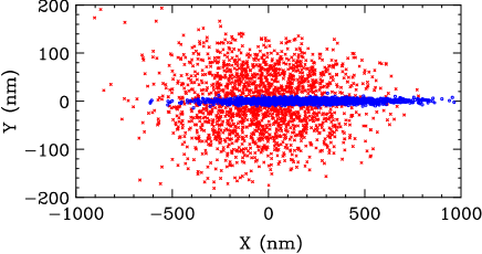
Figure 2: Particle distribution at IP before (red) and after (blue) correction of $\Delta\theta\!=\!10^{-4}$ in QD0.

3 SECOND ORDER KNOBS

Taking into account the small $\sigma_{y}^{*}$ at the NLC, enlargement of IP beam size due to high-order aberrations may also be significant. The FFS sextupoles, octupoles and decapoles may be used to create non-linear correction knobs. Since all of the FFS sextupoles are located at the same phase from IP ($\pi/2\!+\!n\pi$), they create only limited number of second order aberrations at IP. At present, four approximately orthogonal knobs have been constructed using six variable sextupole strengths to generate the projected second order terms at IP: $T_{122}$, $T_{166}$, $T_{342}$ and $T_{364}$. Note that $T_{122}$, $T_{166}$ affect $\sigma_{x}^{*}$ and $T_{342}$, $T_{364}$ change $\sigma_{y}^{*}$. The knobs have been designed using MAD matching routine. Their effect can be analytically estimated by constructing the thin lens second-order matrix containing the desired terms and applying it to the IP phase space.

An example of the second-order correction is presented in Table 5 and Fig. 3, where the strength error $\frac{\Delta K_{2}}{K_{2}}\!=\!10^{-2}$ was applied to the SD0 sextupole. MATLAB-LIAR simulations also showed good compensation in another test, where random strength errors were applied to five FFS sextupoles with rms value of $\frac{\Delta K_{2}}{K_{2}}\!=\!3\!\cdot\!10^{-3}$.

Table 5: DIMAD results (in nm) for $\frac{\Delta K_{2}}{K_{2}}\!=\!10^{-2}$ in SD0.

	$\mathbf{\frac{\Delta K_{2}}{K_{2}}\!=\!0}$	No corr.	Corr.
$\sigma_{x}^{*}/\sigma_{y}^{*}$	253.4 / 3.18	260.1 / 6.02	254.0 / 3.22
$x^{*}/y^{*}$	-27.6/-0.002	-50.5/-0.035	9.6/-0.0003

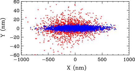
Figure 3: Particle distribution at IP before (red) and after (blue) correction of $\frac{\Delta K_{2}}{K_{2}}\!=\!10^{-2}$ in SD0.

4 CONCLUSION

A set of knobs based on the FFS sextupoles have been designed to correct linear and second-order aberrations at the IP. These knobs have been tested in numerical simulations for several FFS errors and satisfactory compensation has been achieved. Additional high-order knobs are under study. Further simulations will be needed to investigate the error range for an acceptable knob correction and to develop a practical strategy for the beam measurement and knob compensation.

References

- [1] P. Raimondi, A. Seryi, Phys. Rev. Let., 86, p. 3779, 2001.
- [2] P. Raimondi et al., SLAC-PUB-8895, 2001.
- [3] P. Tenenbaum et al., SLAC-PUB-6770, 1995.
- [4] P. Raimondi et al., SLAC-PUB-7955, 1998.
- [5] MAD, http://wwwslap.cern.ch/mad/.
-
[6]
NLC version of DIMAD,
http://www-project.slac.stanford.
edu/lc/local/AccelPhysics/Accel_Physics_index.htm. -
[7]
MATLAB-LIAR,
http://www-project.slac.stanford.edu/lc/
local/AccelPhysics/Accel_Physics_index.htm.