Probabilistic Clustering of Sequences:
Inferring new bacterial regulons by comparative genomics.

Abstract

Genome wide comparisons between enteric bacteria yield large sets of conserved putative regulatory sites on a gene by gene basis that need to be clustered into regulons. Using the assumption that regulatory sites can be represented as samples from weight matrices we derive a unique probability distribution for assignments of sites into clusters. Our algorithm, ’PROCSE’ (probabilistic clustering of sequences), uses Monte-Carlo sampling of this distribution to partition and align thousands of short DNA sequences into clusters. The algorithm internally determines the number of clusters from the data, and assigns significance to the resulting clusters. We place theoretical limits on the ability of any algorithm to correctly cluster sequences drawn from weight matrices (WMs) when these WMs are unknown. Our analysis suggests that the set of all putative sites for a single genome (e.g. E. coli) is largely inadequate for clustering. When sites from different genomes are combined and all the homologous sites from the various species are used as a block, clustering becomes feasible. We predict 50-100 new regulons as well as many new members of existing regulons, potentially doubling the number of known regulatory sites in E. coli.

I Introduction

New microbial genomes are sequenced almost daily, and the first step in their annotation is the elucidation of their protein coding regions. The noncoding regions of the genome can provide clues about gene regulation since they contain various regulatory elements. These elements are generally much smaller and more variable than typical coding regions, and thus harder to identify. Computational methods are needed, since even for E. coli, there are only 60-80 genes for which binding sites and regulated genes are known Robison et al. (1998); Salgado et al. (2000a), whereas protein sequence homology suggests there are $\sim$300 DNA binding proteins Salgado et al. (2000b). Binding sites have been identified experimentally in only 300 of the 2200 regulatory regions of E. coli Salgado et al. (2000a). For important pathogens such as V. cholera, Y. pestis, or M. tuberculosis very little is known about gene regulation from direct experimentation.

Computational strategies for the discovery of regulatory sites began with algorithms Stormo and Hartzell (1989); Lawrence et al. (1993); Bailey and Elkan (1994) which identified sets of similar sequences in the regulatory regions of functionally related groups of genes. More recently, algorithms were proposed to identify repetitive patterns within an entire genome Bussemaker et al. (2000). Here we develop methods for partitioning a large set of putative regulatory sites into clusters based on sequence similarity, with the goal of identifying regulons. That is, we aim to partition the set of sites such that each cluster corresponds to those targeted by the same transcription factor (TF).

Many authors have noted the potential of interspecies comparisons to elucidate regulatory motifs, e.g. Hardison et al. (1997). Generally, a group of functionally related genes in bacteria is pooled to extract common sites within the regulatory regions of these genes, e.g. Gelfand et al. (2000); McGuire et al. (2000). More recent studies McCue et al. (2001); Rajewsky et al. (2002) have shown that when upstream regions of orthologous genes from several suitably related species are compared at once, there is sufficient signal for regulatory sites to be inferred on a gene by gene basis, yielding thousands of potentially new sites. These sites form the data sets on which our algorithm operates.

Previous algorithms that fit WMs can not process genome scale data representing sites from hundreds of TFs simultaneously. Other schemes Bussemaker et al. (2000), not based on WM representations of regulatory sites, are not well suited for processing sites that were inferred from interspecies comparison. Our algorithm partitions the entire set of sites at once, infers the number of clusters internally, and assigns probabilities to all partitions of sequences into clusters. Within this framework, we also derive theoretical limits on the clusterability of sets of regulatory sites.

A set of sites, sampled from a set of unknown WMs, is said to be clusterable if it is possible to infer which sites where sampled from the same WM. If the WMs from which the sites were sampled are known, we have the much simpler classification problem: determining which sites were sampled from which WM. It is important to realize that the cell is performing a classification task since it knows the WMs of the TFs, i.e. the chemistry of the DNA-protein interaction automatically assigns a binding-energy to each site just as a WM assigns a score to each site. However, since we cannot infer binding specificities from a TF’s protein sequence, we face the much harder clustering task. Our theoretical arguments and the available data for E. coli in fact suggest that the set of all regulatory sites in the E. coli genome is unclusterable by itself. However, we also show how this problem can be circumvented by taking into account information from interspecies comparison.

II Model

Protein binding sites in bacterial genomes are commonly described by a WM, $w^{i}_{\alpha}$, which gives the probabilities of finding base $\alpha$ at position $i$ of the binding site Berg and von Hippel (1987). The probabilities in different columns $i$ are assumed independent, which accords well with existing compilations Robison et al. (1998). Motif-finding algorithms Stormo and Hartzell (1989); Lawrence et al. (1993); Bailey and Elkan (1994) score the quality of an alignment of putative binding sites by the information score $I$ of its (estimated) WM:

$$I=\sum_{i,\alpha}w^{i}_{\alpha}\log(w^{i}_{\alpha}/b_{\alpha}),$$ (1)

where $b_{\alpha}$ is the background frequency of base $\alpha$, and the $w^{i}_{\alpha}$ are the WM probabilities, estimated from the sequences in the alignment. The rationale for this scoring function is that the probability of an $n$-sequence alignment with frequencies $w^{i}_{\alpha}$ arising by chance from $n$ independent samples of the background distribution of bases $b_{\alpha}$ is given by $P\approx e^{-nI}$.

Instead of distinguishing sequence-motifs for a single TF against a background distribution, our task is to cluster a set of binding sites of an unknown number of different TFs, i.e. a set of sequences sampled from an unknown number of unspecified WMs. To this end, we consider all ways of partitioning our data set into clusters and assign a probability to each partition.

Figure 1: Two ways of partitioning the same set of sequences into clusters. The rectangle schematically represents the space of all possible DNA sequences of some particular length $l$. The dots denote the sequences in the data set, and the circles indicate which sequences are partitioned together into clusters.

Figure 1 depicts, schematically, two ways of partitioning a set of sequences into clusters. We will assign probabilities to all such partitions. The probability of a partition is the product of the probabilities, for each cluster, that all sequences within the cluster arose from a common WM.

To calculate these probabilities, consider first the conditional probability $P(S|w)$ that a set of $n$ length-$l$ sequences $S$ was drawn from a given WM $w$:

$$p(S|w)=\prod_{s\in S}\prod_{i=1}^{l}w^{i}_{s_{i}},$$ (2)

where $s_{i}$ is the letter at position $i$ in sequence $s$. The probability $P(S)$ that all sequences in $S$ came from some $w$ can be obtained by integrating over all allowed $w$; viz. over the simplex $\sum_{\alpha}w^{i}_{\alpha}=1$ for each position $i$. Lacking any knowledge regarding $w$ we use a uniform prior over the simplex. We obtain

$$P(S)=\int P(S|w)dw={n+3\choose 3}^{-l}\prod_{i=1}^{l}\frac{\prod_{\alpha}n^{i}_{\alpha}!}{n!},$$ (3)

where $n^{i}_{\alpha}$ is the number of occurrences of base $\alpha$ in column $i$. The last factor in Eq. 3 is just the inverse of the multinomial factor that counts the number of ways of constructing a specific vector $(n_{a},n_{c},n_{g},n_{t})$ from $n$ bases, which bears an obvious relation to Eq. 1. High probabilities are thus given to vectors which can be realized in the least number of ways. The factor ${n+3\choose 3}$, counts the number of distinct vectors $(n_{a},n_{c},n_{g},n_{t})$ that can be obtained from $n$ samples.

We can now define for any partition $C$ of a data set of sequences $D$ into clusters $S_{c}$ the likelihood $P(D|C)$ that all sequences in each $S_{c}$ were drawn from a single WM: $P(D|C)=\prod_{c}P(S_{c})$, with $P(S_{c})$ given by Eq. 3. Then the posterior probability $P(C|D)$ for partition $C$ given the data $D$ is

$$P(C|D)=\frac{P(D|C)\pi(C)}{\sum_{C^{\prime}}P(D|C^{\prime})\pi(C^{\prime})},$$ (4)

where $\pi(C)$ is the prior distribution over partitions, which we will assume to be uniform.

Consider the simplest example of a data set of only two sequences with matching bases in $b$ of their $l$ positions. We have $P=2^{b}(1/20)^{l}$ for the probability that the sequences came from the same WM, while $P=(1/16)^{l}$ for the probability that they came from different WMs. $P(C|D)$ will thus prefer to either cluster or separate the two sequences, depending on $b$. In general, the probability distribution $P(C|D)$ will prefer partitions in which similar sequences are co-clustered. The state space of all partitions (the number of which grows nearly as rapidly as $n!$ de Bruijn (1958)) acts as an ’entropy’ which opposes (stable) clustering of similar sequences.

The probability distribution Eq. 4 allows us to calculate any statistic of interest by summing over the appropriate partitions $C$. For instance, to calculate the probability that the data set separates into $n$ clusters, one sums $P(C|D)$ over all partitions that contain $n$ clusters. Analogously, we can calculate the probability that any particular subset of sequences forms a cluster by summing $P(C|D)$ over all partitions in which this occurs. Our clustering framework is novel in that it allows for direct calculations of these quantities. In the implementation section below we describe how we sample $P(C|D)$ and identify significant clusters by finding subsets of sequences that consistently cluster.

Generalizations to data arising from WMs of different lengths and sequences that are not consistently aligned are straightforward and considered below. It is also trivial to incorporate prior information on the number of clusters (e.g. that it should equal the number of TFs).

III Classifiability vs. Clusterability

Correct regulation of gene expression requires that TFs should bind preferentially to their own sites. Associating TFs with WMs, $P(s|w)$ is commonly taken to be the probability that $w$ binds to $s$. Correct regulation thus implies that for a sample $s$ from $w$, we have that $P(s|w)>P(s|w^{\prime})$ for all other TFs $w^{\prime}\neq w$, which we call a classification task. Formally, we are given a set of WMs and a set of sequences sampled from them, and assign each sequence $s$ to the WM from the set that maximizes $P(s|w)$. We define the data to be classifiable when, in at least half of the cases, the WM $w$ which maximizes $P(s|w)$ is the WM from which $s$ was sampled. As mentioned in the introduction, classification is much simpler than clustering a set of sites in absence of knowledge of the set of WMs from which they were sampled.

To quantify clusterability, assume we are clustering $nG$ sequences, that were obtained by sampling $n$ times from each of $G$ different WMs. For each of these WMs we can calculate the probability that $m$ of its $n$ samples co-cluster by summing the probabilities $P(C|D)$ over all partitions $C$ in which $m$, and no more than $m$, samples of $w$ occur together in any of the clusters. We will define the set to be ‘clusterable’ if, for more than half of the $G$ WMs, the average of $m$, $\langle m\rangle>n/2$.

We have performed analytical and numerical calculations that identify under what conditions a data set is classifiable and clusterable. This theory is beyond the scope of this paper and will be reported elsewhere. The results are summarized in Fig. 2.

Figure 2: The critical information score $I$ for clusterability (solid lines) or classifiability (dashed line) as a function of the number of clusters $G$ (shown on a log scale). The solid lines correspond, from top to bottom, to sets of $n=3$, $5$, $10$, and $15$ samples per cluster. The WM length is $l=27$.

Given the information score $I$ (Eq. 1) of a WM, the fraction of the space of $4^{l}$ sequences filled by the binding sites for this WM is $e^{-I}$. One can thus regard $I$ as a measure of the specificity of a WM. Fig. 2 shows the minimal WM specificity necessary to cluster (solid lines) or classify (dashed line) as a function of the number of WMs $G$ and the number of samples $n$ per WM. Fig. 2 shows that $\exp(-I)\propto 1/G$ for classification and $\exp(-I)\approx 1/G^{2}$ for clustering a set of $n=3$ binding sites, with fractional exponents in between these extremes. Thus, all $G$ WMs together consume a fixed fraction of sequence space at the classification threshold (independent of $G$), while it decreases as a function of $G$ at the clusterability threshold. Moreover, there is a significant gap between the requirements for classification vs. clustering, even for large numbers of samples. Thus, clustering is impossible for data sets close to the classification threshold. Results presented below suggest that the collection of E. coli binding sites may well be in this unclusterable regime, where few regulons can be correctly inferred.

However, comparative genomic information can salvage this situation. The putative binding sites of our data sets were extracted by finding conserved sequences upstream of orthologous genes of different bacteria (see below). Such conserved sequence sets are likely to contain binding sites for the same TF, and should be clustered together. Therefore, we can significantly reduce the size of the state space by pre-clustering these conserved sites into so called mini-WMs, and instead of clustering single sequences, we will be clustering these mini-WMs using the same probabilities Eq. 3. This improves clusterability dramatically.

IV Implementation

We have implemented a Monte-Carlo random walk to sample the distribution $P(C|D)$. At every ’time step’ we choose a mini-WM at random and consider reassigning it to a randomly chosen cluster (or empty box). These moves are accepted according to the Metropolis-Hastings scheme Metropolis et al. (1953): moves that increase the probability $P(C|D)$ are always accepted and moves that lower $P(C|D)$ are accepted with probability $P(C^{\prime}|D)/P(C|D)$. Fig. 3 shows an example of a move from a partition $C$ to a partition $C^{\prime}$.

Figure 3: Monte-Carlo sampling of partitions: example of a move from partition $C$ to partition $C^{\prime}$. The dots are sequences and the circles delineate the clusters.

This sampling scheme thus generates ’dynamic’ clusters whose membership fluctuates over time. Clusters may evaporate altogether and new clusters may form when a pair of mini-WMs is moved together. We wish to identify ’significant’ clusters by finding sets of mini-WMs that are persistently grouped together during the Monte-Carlo sampling. Ideally, we would find a set of clusters, each with stable ’core’ members that are present at all times, while the remaining mini-WMs move about between different clusters. Reality is unfortunately more complicated. One finds clusters that are constantly drifting, such that their membership is uncorrelated on long time scales. Other clusters, with stable membership, may evaporate and reform many times. While we can easily sample $P(C|D)$ to obtain significance measures for any given ’candidate cluster’, the rich dynamics of drifting, fusing, and evaporating clusters makes it nontrivial to identify good candidate clusters.

We have experimented with a number of schemes for identifying candidate clusters (see appendix D). One approach is to search for the maximum likelihood (ML) partition that maximizes Eq. 4. This can be done by simulated annealing: we raise $P(D|C)$ to the power $\beta$, increasing $\beta$ over time (in practice $\beta=3$ is large enough). The ML partition gives us a set of candidate clusters. The significance of the ML clusters are then tested by sampling $P(C|D)$. Fig. 4 illustrates this procedure.

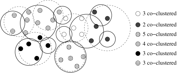
Figure 4: The ML partition obtained by annealing is indicated by the thin dashed circles and the fill patterns of the dots. The thick lines show an alternative partition that may arise during sampling. The number of co-clustering members in this partition are shown on the right for each of the ML clusters.

For each partition encountered during the sampling, we define the number of co-clustering members of a ML cluster as the maximum number of mini-WMs from the ML cluster that co-occur in a single cluster (see Fig. 4). In this way we measure, for each ML cluster, the probabilities $p(k)$ that $k$ of its members co-cluster. Finally, we calculate the minimal length interval $[k_{\rm min},k_{\rm max}]$ for which $\sum_{k=k_{\rm min}}^{k_{\rm max}}p(k)>0.95$. All clusters for which $k_{\rm min}\geq 2$ are deemed significant.

This method is computationally prohibitive for large data sets (because we cannot run long enough to converge all cluster statistics). For larger data sets we measure, using several Monte-Carlo random walks, the probability that each pair of mini-WMs co-clusters. We then construct a graph in which nodes correspond to mini-WMs, and edges between mini-WMs $i$ and $j$ exist if and only if their co-clustering probability $p_{ij}>1/2$. Candidate clusters are now given by the connected components of this graph. The pairwise statistics are then further processed to obtain probabilistic cluster membership. This yields for each mini-WM $i$, the probabilities $p^{i}_{j}$ that mini-WM $i$ belongs to cluster $j$ (see appendix D). We also calculate, for each cluster, the probability distribution $p(k)$ of $k$ of its members co-clustering. Cluster significance is judged from $p(k)$ as described above. Fortunately, there is substantial agreement on the significant clusters among these ways of extracting significant clusters from $P(C|D)$.

After we have inferred the clusters and their members, we can estimate a WM for each cluster. We then classify all mini-WMs in the full data set in terms of these cluster WMs. Finally, we search for additional matching motifs to the cluster WMs in all the regulatory regions of the E. coli genome. Details for all these procedures are described in appendix D.

V Data Sets

Our primary data sets McCue et al. (2001); Rajewsky et al. (2002) consist of alignments of relatively short sequences, i.e. typically $15-25$ bases, that where extracted from upstream regions of orthologous genes in different prokaryotic genomes. Data set McCue et al. (2001) uses the genomes of E. coli, A. actinomycetemcomitans, H. influenzae, P. aeruginosa, S. putrefaciens, S. typhi, T. ferrooxidans, V. cholerae, and Y. pestis. Data set Rajewsky et al. (2002) uses E. coli, K. pneumoniae, S. typhi, V. cholerae and Y. pestis. An example alignment is shown in the upper left of Fig. 5. The available evidence suggests that these alignments either include or substantially overlap a set of binding sites for a TF (or another kind of regulatory site). Our algorithm will have to decide which stretch of bases in each alignment corresponds to the regulatory site. Known binding sites Robison et al. (1998) are between $11$ and $50$ bases long, with a mean of $24.5$ and a standard deviation of just under $10$. We will assume that all binding sites are exactly $27$ bases long, compromising between diluting the signal in the small binding sites, and missing some of the signal in long binding sites. We symmetrically expand the alignments in our data set to length $32$, padding bases from the genomes (see Fig. 5). We would like to treat these sequences as independent samples of a single WM, but for closely related species, this assumption is probably untenable. For alignments from data set McCue et al. (2001) we therefore replace sites from the triplet E. c., Y. p., and S. t., and from the duplet H. i., and A. a. by their respective consensi. For the data set Rajewsky et al. (2002) we only replace the triplet E. c., K. p. and S. t. by their consensus. The ’mini-WMs’ so obtained are the objects that our algorithm clusters. Finally, every time the Monte-Carlo algorithm reassigns a mini-WM to a cluster, it samples over the $6$ different ways of picking a length $27$ window out of the length $32$ alignment, and over both strands (see apppendix C).

Figure 5: Operations on the data sets: Starting from an alignment of variable length, we extend the alignment to length $32$ by padding bases from the genome, and then replace sequences of closely-related species by their consensus. This yields so-called mini-WMs which are the objects that our algorithm clusters. When moved between clusters, a window of length $27$ is sampled from the alignment.

Before clustering these primary data sets we tested the algorithm on a set of experimentally determined TF binding sites in E. coli that was collected in Ref. Robison et al. (1998). We again extended (or cropped) these sequences symmetrically to length 32. After excluding $\sigma$ factor sites and sites that overlap one another by 27 or more bases there are 397 binding sites representing 53 TFs remaining in this test set. See appendix F for details on the pre-processing of this and our other data sets.

For the data set McCue et al. (2001) we removed all alignments that overlap known binding sites or repetitive elements and then took the top 2000 non-overlapping alignments ordered by MAP score. For data set Rajewsky et al. (2002) we also took the top 2000 non-overlapping sites based on significance, but we left sites overlapping known binding sites in this set. Finally, in order to separate new regulons from new sites for TFs with sites in the collection Robison et al. (1998), we aligned all known E. coli sites for each TF into its own mini-WM and added these 56 mini-WMs to the sets McCue et al. (2001) and Rajewsky et al. (2002). Both these sets thus contain 2056 mini-WMs.

We created an additional test set consisting of the $397$ known binding sites from Robison et al. (1998) and the E. coli sequences of the top 2000 unannotated mini-WMs from McCue et al. (2001). As described below, this test verified our prediction that by embedding the $397$ known sites in a larger set of sites, many clusters will fail to be correctly inferred.

VI Results

We used the test-set of 397 known binding sites in several ways. First, we sampled $P(C|D)$ and measured, for each factor, how well its sites cluster. That is, we measured the co-clustering distribution $p(k)$ for each TF. Using the significance threshold described above, we found significant clusters for 24 of the 53 TFs. Twenty two TFs have 3 or fewer sites in the test set and, with the exception of trpR, their sites did not cluster significantly. As a better test of our algorithm, we compared the clusters inferred from annealing this data set with the site annotation. We performed two annealing runs to identify a ML partition, and then performed sampling runs to test the significance of these maximum likelihood clusters. We found that, in general, there is good agreement between the annotation and the clusters inferred by annealing. For 17 of the 24 TFs that form significant clusters there was an analogous significant cluster obtained by the annealing. The full results are in appendix G. We have also found that the likelihood $P(C|D)$ for the partition obtained in all annealing runs is significantly higher than that obtained when the sites are partitioned according to their annotation. Thus we feel that the clustering for this data set can not be improved within our scoring scheme. In short, our algorithm recovers almost half of all regulons for which binding sites are known, and the large majority of regulons for which there are more than three sites known.

We sampled $P(C|D)$ for the 2397 site test-set and found that, as predicted, many clusters are lost (only 9 of 24 significant clusters remain). Several of those that remain where reinforced by the presence of additional unannotated sites in the supplemental set of 2000. (More samples improves clusterability as we have seen in the clusterability section.) For this larger data set, the total number of clusters fluctuates around 350 during the run, but only $\sim 5$% of these are significant. This suggests that most E. coli binding sites are in the unclusterable regime, and that comparative genomic information is essential to effectively cluster. We also performed simulations with ’surrogate’ data sets that further support this claim. For each cluster of known binding sites, we calculated the information score $I$ of its WM and created 4 random WMs with equal $I$. By drawing samples from each of these, we ‘scaled up’ the set of known binding sites and clusters by a factor of 5, to correspond to the the estimated number of TF in E. coli. In sampling $P(C|D)$ for this set, we found that less than 10% of the clusters are correctly inferred.

For the larger data sets from McCue et al. (2001); Rajewsky et al. (2002), that are our main interest, repeated annealing and sampling runs indicated that both the annealed state and the significance statistics are not fully converged within our running times ($10^{10}$ steps, taking a week on a workstation per run). We therefore extracted significant clusters via pair statistics as described above, which did converge and allowed us to assign error-bars to all pair statistics. For the data set McCue et al. (2001), there were $365\pm 5$ clusters on average and the connectivity graph gave 274 components containing 1139 out of 2056 mini-WMs. Thus, about half of the data set clusters stably, while the other half moves in and out of the $\sim$100 unstable clusters. There were 115 significant clusters comprising, 645 mini-WMs. Of the $115$ significant clusters, 21 contained, as one of its member mini-WMs, the alignment of a set of known binding sites for the same TF from Robison et al. (1998). These clusters thus contain new sites for known regulons. The other 94 clusters correspond to new putative regulons some examples of which are described below.

It is interesting to calculate the cluster information scores, $I$, to compute the fractions, $e^{-I}$, of sequence space occupied by our clusters. Summing these volumes, we find that approximately 1% of the space is filled by the top 45 clusters, the top 80 clusters fill 10% of the space, and all our 115 significant clusters fill 39% of the space. This again supports the idea that the set of all WMs is close to the classification boundary: their binding sites fill almost the entire sequence space.

For the data set Rajewsky et al. (2002) there are $275\pm 4$ clusters on average during the sampling. The connectivity graph has 176 clusters containing 726 mini-WMs. There were 65 significant clusters (containing 398 mini-WMs), of which 25 correspond to known regulons. With respect to the sequence space volume filled by the WMs of these clusters: 1% of the space is filled by the first 30 clusters, 50 clusters fill 10% of the space, and the full set of 65 WMs fills about 50% of the sequence space.

VII Examples

Table 1 contains a synopsis of some of predicted new regulons we have examined in detail from the data set McCue et al. (2001). Primary cluster membership is noted along with additional sites that can be found by scanning the cluster WM over the full data set and all regulatory regions of E. coli. The complete lists are on our web site website .

Table 1: Sample clusters from the data set McCue et al. (2001). The cluster rank is by WM information score. The defining operons come in three categories; Those with member sites in the data set on which the algorithm was run (bold). Those with sites in McCue et al. (2001) that match the WM (normal font), and those that were found by scanning the regulatory regions of E. coli (italics). Multiple genes within an operon are separated by a / or by multiple capitals at the end of the gene name. Operons separated by a comma indicates that the site fell between divergently described genes.

cluster name	rank	defining operons
thiamin biosynthesis	0	thiCEFGH tpbA/yabKJ thiMD thiL
gntR/idnR regulon	1	idnK,idnDOTR gntKU gntT b2740 edd/eda
elongation factor	2	tufB
ribonucleotide reductase	3	nrdAB nrdDG nrdHIEF
?	4	coaA tgt/yajCD/secDF yegQ b3975 tpr yeeO
stem-loop/attenuator	5	yhbc/nusA/infB mutM arsRBC yhdNM
repair ?		nadA/pnuC lig ptsHI/crr rbfA/truB/rpsO
ntrC regulon	11	glnK/amtB cmk/rpsA glnALG glnHPQ
		narGHJI hisJQMP
ribosomal protein attenuation	15	thdF fabF recQ tsf pnp pyrE himD
anaerobic oxidation	16	cydAB appCB yhhK,livKHMGF
		torCAD,torR ansB/yggM ybbQ yiiE
fatty acid biosynthesis	17	fabA b2899(yqfA) fabB fabHDG
cell envelope	25	pcnB/folK pssA dksA/yadB yaeS
replication ?		mreCD/yhdE/cafA sanA cmk/rpsA
alkaline phosphatase	26	yaiB/phoA/psiF, ddlA dnaB/alr
peptidoglycan		creABCD iap avtA
transport	37	abc,yaeD cadBA araFGH,yecI celABCDF
		citAB,citCDEF agaBCD tauABCD
fruR regulon	71	fruR fruBKA epd yggR
Fe-S radicals	85	metK,yqgD ftn pykA yheA/bfr

Our thiamin cluster is an example of a predicted new regulon that has recently been experimentally confirmed. A comprehensive review of thiamin biosynthesis in prokaryotes Begley et al. (1999) places the genes from the three operons of our thiamin cluster into a single pathway, together with the four single genes: thiL, thiK, dxs (yajP), and thiI (yajK). A recent paper Miranda-Rios et al. (2001) shows that the three thiamin operons share a common RNA stem-loop motif which is responsible for posttranscriptional regulation. It is precisely a portion of this motif that we cluster. A fragment of this structure also occurs just upstream of translation start in thiL. For the remaining genes thiK, dxs, and thiI, there are no putative sites in the data set McCue et al. (2001).

Besides the main gluconate metabolism pathway, a second pathway that utilizes input from the catabolism of L-idonic acid has recently been reported Bausch et al. (1998) and corresponds to our second cluster. The first two operons (idnK, idnDOTR) code for the enzymes that import L-idonate and convert it to 6-P-gluconate. The operon gntKU contains a a gluconokinase, which catalyzes the same reaction as the idnK protein, and a low-affinity gluconate permease. b2740 is a gene of unknown function which belongs to the family of gluconate transporters. Finally, gntT is a high affinity gluconate permease. Additional sites were found upstream of the edd/eda operon, which encode the key enzymes of the Entner-Doudoroff pathway Peekhaus and Conway (1998a). Ref Bausch et al. (1998) suggests that idnR both upregulates the L-idonate catabolism genes and represses gntKU and gntT when growing on L-idonate. This suggest our sites may bind indR. However, there are two sites upstream of gntT, which are annotated as gntR sites Peekhaus and Conway (1998b), which are also part of our cluster.

The pathway for ribonucleotide reduction to deoxyribonucleotides is pictured on p. 591 of Neidhardt (1996) and includes the first two operons of our like named cluster. We did not find sites in the regulatory regions of the other two genes in this pathway (ndk, dcd). Scanning of the genome with the WM inferred from the nrdAB and nrdDG sites reveals an additional 3 (weaker) sites upstream of the nrdHIEF operon. The nrdEF genes are annotated as a cryptic ribonucleotide reductase. The regulation of our two primary operons (nrdAB, nrdDG) is known to be complex and includes an fnr site upstream of nrdD (which we correctly clustered with other fnr sites), and additional fis, dnaA, and unattributed sites upstream of nrdA Jacobson and Fuchs (1998). The nrdA site in our cluster is a new site, located down stream of transcription start. Since nrdA is down regulated during anaerobiosis, and nrdD is essential for anaerobic growth, we would guess that our sites are involved in the switch.

The estimated WM of cluster 5 has a prominent inverted repeat sequence as its consensus:
AAAAacCC***TT***GGGGgTTTTTT,
and has over 20 matches in the genome. These sites may correspond to an RNA secondary structure, possibly involved in attenuation. There is no clear predominant functional theme to the genes in our cluster 5. Noteworthy are sites upstream of the arsenic resistance operon (arsRBC), the crr regulator of a multidrug efflux pump, and the ydnM (zntR) regulator for Pb(II), Cd(II), and Zn(II) efflux. Also, two genes involved in DNA repair occur (MutM, lig).

The sites in cluster 15 occur upstream of genes whose proteins are involved in RNA modification (thdF, pnp), recombination (recQ, himD) and translation (tsf). More strikingly, 6 out of 7 of these sites occur downstream of genes coding for ribosomal protein subunits and one RNase. For 5 of these, there is evidence Ecocyc that our site falls within a transcription unit, i.e. that the genes upstream and downstream of our site are co-transcribed. It seems likely that these sites are involved in either attenuation or else translational regulation.

E. coli has a rich repertory of respiratory chains that are built from a variety of electron donors and acceptors, see p. 218 Neidhardt (1996). One of our clusters (16) involves two homologous cytochrome operons cydAB and appCB (cyxAB), which transfer electrons to oxygen and are mainly active during anaerobic conditions. The torACD operon (divergently transcribed with its regulator torR) transfers electrons to trimethylamine N-oxide. There is a third cytochrome complex, cyoABCD, with different specificity, that is not linked to this cluster. Other operons in this cluster, such as livKHMGF, which is involved in amino acid import, and ansB, which catalyzes asparagine to aspartate conversion, seem unrelated but are divergently transcribed with genes of unknown function. However, Ref. Jennings and Beacham (1990) and p. 366 Neidhardt (1996) suggest that ansB, can also provide fumarate as a terminal electron acceptor. AnsB is strongly upregulated during anaerobic conditions and has known crp and fnr sites. The ansB site in our cluster is different from these sites.

Cluster number 17 corresponds to the fatty acid biosynthesis regulon with TF yijC (fabR) that was identified in McCue et al. (2001). Our cluster contains the sites they found upstream of fabA and b2899. Additionally, we found WM matches upstream of the related genes fabB and fabHDG. Other operons with lower quality sites in the cluster include the mglBAC operon (methyl-galactoside transport), clpX (component of clpP serine protease), and the putative peptidase b2324.

We are unable to guess the functional role of the binding sites clustered in cluster number 25. Some of the genes have functionalities related to the cell envelope and membrane (pssA, yaeS, mreCD, sanA) and some seem involved in replication (dskA, cafE). However, these functions seem rather diverse.

For cluster 26, we find sites upstream of genes involved in peptidoglycan biosynthesis (alr, ddlA, avtA, mrcB), and genes that are known to be regulated in response to phosphate starvation (creABC, iap, phoA/psiF). In particular, alkaline phosphatase (phoA) is upregulated more than 1000-fold and accounts for as much as 6% of the protein content of the cell during phosphate starvation, see p. 1361 Neidhardt (1996). Since alkaline phosphatase is active in the periplasm, it seems conceivable that peptidoglycan synthesis is down-regulated when phoA is expressed at such high levels.

Additional clusters with obvious common functionality include: cluster 85 for Fe-S radical synthesis Cheek and Broderick (2001), and the large cluster 37 which contains several PTS and other transport systems. Cluster 71 contains sites that overlap binding sites for the fructose repressor fruR. These were clustered separately from the known fruR sites because of a systematic shift, larger than the range our algorithm scans, between how they were given in McCue et al. (2001) and the annotated fruR sites. Similarly, cluster 11 contains sites that overlap binding sites for the nitrogen fixation regulator ntrC (glnG).

Apart from these putative new regulons, our web site website has an additional 270 unique sites that cluster with WMs of known TFs. Summing their membership probabilities, this corresponds to an expected 135 new binding sites. The website also provides information for each E. coli gene separately: inferred regulatory sites upstream of the gene and the cluster memberships of these sites.

The clusters inferred from the data Rajewsky et al. (2002) are also on our web site website . We have not yet evaluated their functional significance, but some of them correspond to clusters that we also found in the data of McCue et al. (2001), e.g., the thiamin cluster reappears.

VIII Discussion

We introduced a new inference procedure for probabilistically partitioning a set of DNA sequences into clusters. Currently, the algorithm assumes all WMs to be of a fixed length, but prior information about site lengths, their dimeric nature, and the length of spacers between dimeric sites could be easily included. One could also extend the hypothesis space on which the algorithm operates: one may assume that only some fraction, rather than all, of the sequences are WM samples, while the rest should described by a ‘background’ model. This would, for instance, be appropriate for analyzing entire upstream regions. In all these generalizations, the algorithm would still assign probabilities to sets of sequences belonging to a single TF. This essentially Bayesian approach should be contrasted with approaches, e.g. Bussemaker et al. (2000); Stormo and Hartzell (1989), in which ’promising’ motifs are selected based on how unlikely it is for them to occur under some null hypothesis of randomness.

By applying our algorithm to data sets McCue et al. (2001); Rajewsky et al. (2002) of putative regulatory sites extracted from enteric bacteria, we predicted $\sim 100$ new regulons in E. coli, containing $\sim 500$ new binding sites, and predicted $\sim 150$ new binding sites for known TFs. The functionality of many of the predicted new regulons is supported by the fact that their sites are found upstream of genes that are clearly functionally related. Even if there is no common theme in the annotation of the genes controlled by the sites, our significance measures suggest that a large fraction of the clusters is functional: the data-sets contain only conserved sites upstream of orthologous genes in different organisms, and a highly significant association of groups of such sites was found. We note that our set is a considerable augmentation of the $\sim 400$ non-$\sigma$ sites that are known experimentally. Analysis of some our clusters shows that included in our predicted regulons in addition to TF binding sites, are RNA stems controlling translation, and even termination motifs.

The clusters and sites resulting from our genome wide analysis of regulatory motifs allows for a more quantitative evaluation of the global structure of regulatory networks in bacteria. The regulatory network is often imagined as a rather loosely coupled collection of ’modules’, where each regulon controls a set of genes with closely linked functionality (although, many exceptions of course exist, such as the structural TFs fis, ihf, etc.). Our predicted regulons are often much less orderly. In several cases, some but not all genes of a well studied pathway entered the regulon. In other cases, a regulon contains sets of sites for genes of two or three clearly distinct functionalities for which no regulatory connection is known. Our overall impression is of a more haphazard regulatory network than traditionally imagined.

Finally, we have emphasized the distinction between classifying and clustering a set of binding sites. We have argued that the TFs of a cell are essentially solving a classification task, and that inferring regulons from the set of binding sites of a single genome may well be impossible in principle. There are also evolutionary arguments that support this claim. Like any piece of DNA, binding sites are subject to random mutations. The more specific binding sites are, the more likely they are to be disrupted by mutations. Evolution will thus naturally drive TFs and their binding sites to become as unspecific as possible van Nimwegen et al. (1999); Sengupta et al. (2002) within the constraints set by their function. That is, evolution will drive the set of binding sites toward the ’classification threshold’ where they become unclusterable. The situation is reminiscent of the situation in communication theory, where optimally coded messages look entirely random to receivers that are not in possession of the code. Information from comparative genomics is thus essential for the inference of regulons from genomic data, and as the number of sequenced genomes grows, so will our algorithm’s ability to discover new regulons.

Appendix A The Weight Matrix Representation of Binding Sites

In this section we briefly explain which assumptions are implied in the weight matrix (WM) representation of transcription factor binding sites. Transcription factors (TFs) will bind specifically to certain DNA segments in the genome. We wish to mathematically represent the sequence features, shared by these segments, that are responsible for the specific recognition by the TF. It is generally assumed Berg and von Hippel (1987) that the binding energy $E(s)$ of the TF to a DNA sequence segment $s$ can be written as a sum of binding energies $E_{i}(s_{i})$ for the different bases in the segment:

$$E(s)=\sum_{i=1}^{l}E_{i}(s_{i})$$ (5)

The probability $P_{\rm bound}(s)$ that the TF binds to a sequence $s$ in the genome is then proportional to

$$P_{\rm bound}(s)\propto e^{\beta E(s)},$$ (6)

where $\beta=1/(kT)$. We now further assume that binding sites for a particular TF are distinguished from all other DNA segments in that they have higher binding energies. That is, binding sites are characterized by having some expected binding energy $\langle E\rangle$ which is substantially higher than the expected binding energy of random sequences. Under these assumptions, the probability distribution $P(s)$ that segment $s$ is a binding site for the TF is given by the maximum entropy distribution under the condition $\langle E(s)\rangle=\langle E\rangle$,

$$P(s)=\frac{e^{\lambda E(s)}}{\sum_{s^{\prime}}e^{\lambda E(s^{\prime})}}=\prod_{i=1}^{l}\frac{e^{\lambda E_{i}(s_{i})}}{\sum_{\alpha}e^{\lambda E_{i}(\alpha)}},$$ (7)

where the sum over $s^{\prime}$ is over all length-$l$ sequences, and the sum over $\alpha$ is over the four bases. The Lagrangian multiplier $\lambda$ is chosen such that $\sum_{s}E(s)P(s)=\langle E\rangle$. If we define the WM

$$w^{i}_{\alpha}=\frac{e^{\lambda E_{i}(\alpha)}}{\sum_{\alpha^{\prime}}e^{\lambda E_{i}(\alpha^{\prime})}},$$ (8)

then we can represent TFs by WMs, and write for the probability $P(s|w)$ that $s$ is a binding site for the TF represented by $w$ as

$$P(s|w)=\prod_{i=1}^{l}w^{i}_{s_{i}}.$$ (9)

In summary, under the assumption that the binding energy of a TF to a DNA segment $s$ can be written as a sum of the binding energies of the individual bases in $s$ to the TF, and assuming that binding sites for a TF can be characterized by having a certain expected binding energy $\langle E\rangle$, we can represent TFs by WMs $w$. For each length-$l$ DNA segment $s$, the probability of this segments being a binding site for TF $w$ is simply given by a product of the WM probabilities of the individual bases, as described above.

A.1 Information Scores

If we have an alignment of $n$ length-$l$ sequences, with $n^{i}_{\alpha}$ occurrences of base $\alpha$ at position $i$, we can ask for the probability $P(n^{i}_{\alpha}|b_{\alpha})$ of observing these base counts under the assumption that all these sequences are random, with probabilities $b_{\alpha}$ for base $\alpha$ occurring at each position. This probability is given by

$$P(n^{i}_{\alpha}|b_{\alpha})=\prod_{i=1}^{l}n!\prod_{\alpha}\frac{(b_{\alpha})^{n^{i}_{\alpha}}}{n^{i}_{\alpha}!}.$$ (10)

If we use the Stirling approximation for the factorials (valid for $n$ moderately large):

$$\log(n!)\approx n\log(n)-n,$$ (11)

and write for the WM entries

$$n^{i}_{\alpha}=nw^{i}_{\alpha},$$ (12)

we obtain

$$P(n^{i}_{\alpha}|b_{\alpha})=\exp\left[-n\sum_{i,\alpha}w^{i}_{\alpha}\log(w^{i}_{\alpha}/b_{\alpha})\right]\equiv e^{-nI},$$ (13)

where we have defined the WM information score $I$ as

$$I=\sum_{i,\alpha}w^{i}_{\alpha}\log(w^{i}_{\alpha}/b_{\alpha}).$$ (14)

Thus, the higher the information score of the observed alignment, the less likely it is to occur by chance from sampling random bases. This is the main reason that most authors use the information score to assess the quality of alignments of putative binding sites.

Obviously, for small $n^{i}_{\alpha}$ and especially if some of the $n^{i}_{\alpha}$ become zero, the Stirling approximation breaks down, and it would be best to use the exact (10). The information score can thus best be defined as

$$I=-\frac{\log[P(n^{i}_{\alpha}|b_{\alpha})]}{n}$$ (15)

from the exact expression for all values of $n$.

Appendix B The Partition Likelihood Function

We recall that the probability $P(S|w)$ that all sequences of a set $S$ were drawn from a WM $w$ is given by

$$P(S|w)=\prod_{s\in S}\prod_{i=1}^{l}w^{i}_{s_{i}},$$ (16)

where $s_{i}$ is the base occurring at position $i$ in sequence $s$. To calculate the probability $P(S)$ that all sequences in a set $S$ were drawn from the same WM, independent of what this WM may be, we integrated over the hypersimplex

$$\sum_{\alpha}w^{i}_{\alpha}=1,\;\forall i\in\{1,2,\ldots l\}.$$ (17)

Generally, one would have to choose some integration measure $\pi(w)$ on this space (which is equivalent to choosing a prior). We then have

$$P(S)=\int\,\pi(w)P(S|w)dw.$$ (18)

We chose a uniform prior that normalizes the integrals

$$\pi(w)=(3!)^{l}.$$ (19)

In cases where the sampling distribution is multinomial (as it is in our case), it is customary to use so-called Dirichlet priors

$$\pi(w)=\prod_{i,\alpha}(w^{i}_{\alpha})^{\lambda_{\alpha}-1}.$$ (20)

Demanding a prior that is invariant under scale transformations of the $w^{i}_{\alpha}$, one would arrive at $\lambda_{\alpha}=0$. There are good arguments for suggesting that this corresponds to a complete ignorance prior for $w$ Jaynes (1983). It is also easy to derive that setting $\lambda_{\alpha}$ to some value larger than zero is equivalent to adding $\lambda_{\alpha}$ counts for each letter $\alpha$ to the data. For this reason, the $\lambda_{\alpha}$ are also referred to as pseudo-counts. We interpret our use of $\lambda_{\alpha}=1$ as representing the knowledge that it is definitely possible for each base $\alpha$ to occur at each position. That is, we known $w^{i}_{\alpha}>0$ for all $\alpha$. In any case, these are subtleties that hardly affect the inference. For instance, some authors (e.g., ref. Lawrence et al. (1993)) prefer to choose $\lambda_{\alpha}$ proportional both to the frequency of $\alpha$ in the “full” data set (being for instance the genome or all of its intergenic regions) and proportional to the square root of the number of sequences in the alignment. We, however, fail to see how a representation of our prior knowledge should depend on the data set, nor why WMs should a priori be likely to be skewed toward bases that have a higher frequency of occurrence in the full genome or its upstream regions (which consist mostly of DNA that is not part of a binding site). Still, we have experimented with such priors and noticed that the clustering behavior is hardly affected at all. We thus chose to use the uniform prior since it is simpler, and more easily justifiable theoretically.

Finally, some remarks on the importance of the integration over $w$ in calculating the probability of a cluster. First of all, it is of course simply a matter of probability theory that if we want to calculate the probability that all sequences in the cluster came from the same WM, in absence of any knowledge about this WM, we have to integrate over $w$. However, one may for instance be tempted to assign a “score” to each cluster by finding the WM $w^{*}$ that maximizes the likelihood $P(S|w^{*})$ that all sequences in the cluster came from this WM. One would find

$$P(S|w^{*})=\prod_{i=1}^{l}\prod_{\alpha}\left(\frac{n^{i}_{\alpha}}{n}\right)^{n^{i}_{\alpha}},$$ (21)

where the maximum likelihood (ML) WM has entries $(w^{*})^{i}_{\alpha}=n^{i}_{\alpha}/n$.

The problem with an approach like this is that, trivially, the partition in which each sequence forms its own cluster will be the partition that maximizes the score. That is, for single-sequence clusters one can always find a WM that gives rise to that sequence with probability $1$. Obviously, we would not want this totally “unclustered” state to have the highest score. The source of the problem is that to obtain these ML scores, one has to choose all WMs such that the likelihood is maximized. The more clusters there are in the partition, the more WMs have to be set to their ML values. One thus allows oneself to optimize over more degrees of freedom for a partition with many clusters than for a partition with a small number of clusters. One then might be tempted to introduce some kind of “penalty” per degree of freedom that has to be optimized to obtain the ML score. However, these problems are solved automatically when one applies probability theory correctly, that is, when one performs the integration over $w$.

B.1 Estimating WM Entries

Given an alignment of sequences that we believe to be sampled from the same WM, we would like to estimate the WM entries $w^{i}_{\alpha}$ from which these sequences were sampled. In general we have for the expected WM entry $\langle w^{i}_{\alpha}\rangle$

$$\langle w^{i}_{\alpha}\rangle=\frac{\int w^{i}_{\alpha}P(S|w)\pi(w)dw}{\int P(S|w)\pi(w)dw},$$ (22)

where the integral is again over the hypersimplex, and $\pi(w)$ is again the prior on this space. With the general Dirichlet prior one finds

$$\langle w^{i}_{\alpha}\rangle=\frac{n^{i}_{\alpha}+\lambda_{\alpha}}{\sum_{\beta}n^{i}_{\beta}+\lambda_{\beta}}.$$ (23)

With our prior $\lambda_{\alpha}=1$, we thus have $\langle w^{i}_{\alpha}\rangle=(n^{i}_{\alpha}+1)/(n+4)$.

B.2 Relation to the Gibbs Sampler

Consider a situation in which there only two clusters: one very large “reservoir” cluster and one small cluster (which contains the estimated alignment of binding sites for a single TF). Under our model, this partition has a certain probability $P$. We are now interested in calculating the change $P\rightarrow P^{\prime}$ in that probability when a single sequence is moved out of the reservoir cluster into the smaller cluster. With $n^{i}_{\alpha}$, the number of bases $\alpha$ in column $i$ before the move and $N_{\alpha}$ the number of bases $\alpha$ in the “background reservoir” (which is assumed to have equal base frequencies $b_{\alpha}$ in each column), this is given by

$$P^{\prime}=P\prod_{i=1}^{l}\frac{n^{i}_{\alpha}+1}{n+4}\frac{N+3}{N_{\alpha}}\equiv PQ.$$ (24)

In the limit of $N$ goes to infinity the factor $Q$ reduces to

$$Q=\prod_{i=1}^{l}\frac{n^{i}_{\alpha}+1}{(n+4)b_{\alpha}}=\prod_{i=1}^{l}\frac{\langle w^{i}_{\alpha}\rangle}{b_{\alpha}},$$ (25)

with $b_{\alpha}$ the background base frequencies and $\langle w^{i}_{\alpha}\rangle$ the expected WM entries based on the $n$ members of the smaller cluster prior to the addition of the new sequence. This factor $Q$ is precisely (assuming uniform pseudo-counts) the scoring that is used by the Gibbs sampler algorithm. Thus, under the assumption that the data set consists of a large set of “background” sequences plus a set of binding sites for a single TF, our scoring reduces to the scoring of Gibbs sampler. Note, however, that assuming a single cluster plus background is of course not correct for data sets of the type that we cluster in the paper.

B.3 Prior on the Space of Partitions

In the paper, we are using a uniform prior over all possible partitions. The argument for using such a prior is that it is the maximum entropy prior with respect to the space of partitions. In absence of any prior knowledge about which partitions are more or less likely, a uniform prior is the least “assuming” of any prior. We note, however, that there are some subtleties with this reasoning. Instead of saying that we are a priori completely ignorant regarding which partition is more or less likely, it may seem that we may just as well have said that we are completely ignorant regarding the number of clusters that underlie the data. These two statements are mutually inconsistent, however. The number of ways of partitioning a set of $N$ objects into $n$ subsets is given by a so-called Stirling number of the second kind $S^{N}_{n}$. The total number of ways of partitioning a set of $N$ objects into subsets is

$$b_{N}\equiv\sum_{n=1}^{N}S^{N}_{n}.$$ (26)

A uniform prior over the partitions thus corresponds to a probability distribution

$$P_{n}=\frac{S^{N}_{n}}{b_{N}}$$ (27)

over the number of clusters $n$. This distribution has, for large $N$, a relatively sharp peak at some value of $n$. Therefore, complete ignorance regarding the partition “induces” knowledge regarding the number of clusters.

We could of course have chosen a uniform prior over the number of clusters, thereby increasing the relative weight of partitions with cluster numbers that can be realized in fewer ways. We are, however, not trying to infer the cluster number, we are inferring which particular partitions are most likely. We therefore feel that a uniform prior of partitions is the most relevant for our purposes.

Appendix C Monte Carlo Sampling

In this section we explain in more detail how our Monte Carlo sampling is implemented. First of all, we want to implement a move set that would sample all partitions of our set of mini-WMs equally often if the probability distribution $P(D|C)$ were constant. That is, we want to implement a move set that respects the uniform prior. This can be done as follows.

Let our data set contain $N$ mini-WMs and imagine that we have $N$ boxes. A clustering state can be specified by assigning the $N$ mini-WMs to the $N$ boxes (leaving some boxes empty of course). There are $N^{N}$ such states. This state space (call it $X$) can be easily uniformly sampled by, at each time step, picking one of the $N$ objects at rando, and moving it to one of the $N-1$ other boxes, which is also to be chosen at random. However, a uniform sampling of $X$ does not correspond to a uniform sampling of the space of partitions. For each possible partition $C$ of the data set, there is a multitude of states in the state space $X$ that correspond to this partition $C$. To be precise, for a partition $C$ containing $n$ clusters there are $N!/(N-n)!$ states in the state space $X$ that correspond to the same partition $C$ (all ways of permuting the $N$ boxes, divided by all ways of permuting the empty boxes). Therefore, partitions with $n+1$ clusters have $N-n$ times as many states in $X$ as partitions with $n$ clusters. We thus bias the move-set on $X$ such that the rate of moving from a state with $n+1$ clusters to a state with $n$ clusters is $N-n$ times as high as the backward rate. This will ensure a uniform sampling of the space of partitions.

A second issue that the Monte Carlo walk has to deal with is the aligning of the mini-WMs with respect to each other. As mentioned in the text, all our mini-WMs are $32$ bases long, while we assume that the binding sites are $27$ bases long. There are six ways of placing a length $27$ window over the length $32$ mini-WM. Every time a mini-WM is moved during the random walk, we sample over these six possible shifts and over both strands of the DNA (leading to $12$ possible ways of picking the “site” from the length $32$ window). This sampling is done by so-called importance sampling.

Assume that we want to consider moving mini-WM $m$ from a cluster containing the set of sequences $S$ into a cluster containing the set of sequences $S^{\prime}$. Let $P(S^{\prime})$ be the probability of the set $S^{\prime}$ without $m$ added, and let $P(S^{-})$ be the probability of the set of sequences $S$ when $m$ is removed. Further, let $P(S^{\prime},i,s)$ be the probability of the cluster $S^{\prime}$ when mini-WM $m$ is added, with a shift $i$ and using strand $s$ (where $i$ runs from $0$ to $5$, and $s$ is either positive or reverse complement). Finally, let $P(S^{-},i,s)$ be the probability of cluster $S$ with $m$ added at shift $i$ and strand $s$. We then define

$$Z=P(S^{\prime})\sum_{i=0}^{5}\sum_{s\in\{+,-\}}P(S^{-},i,s),$$ (28)

and

$$Z^{\prime}=P(S^{-})\sum_{i=0}^{5}\sum_{s\in\{+,-\}}P(S^{\prime},i,s).$$ (29)

The move of $m$ from $S$ to $S^{\prime}$ is accepted when $Z^{\prime}\geq Z$, and accepted with probability $Z^{\prime}/Z$ when $Z^{\prime}<Z$. After $m$ is assigned to either $S$ or $S^{\prime}$, one of the $12$ strand/shift combinations is sampled with probability $P(S^{-},i,s)/Z$ (or $P(S^{\prime},i,s)/Z^{\prime}$ depending on which cluster $m$ was assigned to). This extension of the move set will sample over all possible shift and strand combinations that the clusters can take.

With this move set, it still seems that stable clusters may get “trapped” into an unfavorable positioning of their window. That is, assume that some subset of mini-WMs has high similarity and can form a stable cluster. Let us also assume that these sites are not shifted with respect to each other, so that with high likelihood an alignment will be sampled in which all mini-WMs in the cluster occur with the same shift. Still, one may choose different values for this shift, i.e. the alignment may contain bases $0$-$26$, or bases $1$-$27$, etc. Once one of these shifts is chosen our move set makes it very unlikely for the cluster to revert to another shift unless it evaporates. To defeat clusters getting trapped in a particular shift this way we implemented one more move: the “coherent shift”. In this move, we sample, according to their probability, from all ways of shifting all mini-WMs in the cluster by the same amount. This sampling is performed (with probability $p$) on the cluster that contains the mini-WM that was randomly selected to be reassigned. In our implementation we chose $p=0.05$. The behavior of the algorithm is insensitive to this value. One only has to make sure that the coherent shift is tried at least once during the lifetime of a typical cluster.

Finally, we altered the probability $P(S)$ for clusters consisting of a single mini-WM. For those single mini-WM clusters, we interpret the mini-WM as stemming from a random background distribution as opposed to it consisting of samples from a binding sites. That is, instead of a score $4^{ln}$ (with $l$ the length and $n$ the number of sequences in the mini-WM) we use a probability

$$P=\prod_{s\in S}\prod_{i=1}^{l}b_{s_{i}},$$ (30)

where $S$ is the set of sequences that make up the mini-WM, and $b_{\alpha}$ is the back ground frequency of letter $\alpha$ in the upstream regions. It must be admitted that this is somewhat of a hybrid procedure. If we had really wanted to consider a hypothesis space in which some of the mini-WMs can be “background” sequences as opposed to WM samples, then we should have chosen a prior on the space of partitions that properly reflects this.

A typical Monte Carlo run has on the order of $10^{10}$ (considered) moves. It takes less than $10^{9}$ moves to reach “equilibrium”. That is, for the first $10^{8}-10^{9}$ time steps the sampled values of $P(D|C)$ are decreasing, whereas they fluctuate around some fixed value after $10^{9}$ time steps. For the data set from ref. McCue et al. (2001) this equilibrium value is given by

$$\log[P_{\rm ss}]\approx 0.93\log[P_{\rm uc}],$$ (31)

where $P_{\rm ss}$ is the steady-state value of the probability $P(D|C)$ and $P_{\rm uc}$ is the probability of the entirely unclustered state where each mini-WM forms a cluster by itself.

C.1 Annealing

The annealing is performed by raising all probabilities to the power $\beta$ and slowly raising $\beta$ over time. That is, a move form partition $C$ to $C^{\prime}$ is accepted with probability $[P(D|C^{\prime})/P(D|C)]^{\beta}$.

We experimented with different annealing schedules, and a simple linear increase of $\beta$ with time gives the best results. We let the algorithm run at $\beta=1$ for $10^{8}$ steps and then start increasing $\beta$ linearly with time, such that $\beta\approx 3$ in the end phase of the annealing. The last $5*10^{7}$ time steps are then done with a very high value of $\beta$, essentially only accepting moves that increase the probability $P(D|C)$, thereby leading to a locally optimal partition at the end of the run.

Appendix D Extracting Significant Clusters

The simplest way in which we could use our assignment of probabilities to partitions to extract clusters is by treating the probabilities simply as a “scoring” function and attempting to find a partition of optimal score. One could for instance use hierarchical clustering:

1. Start with each mini-WM forming its own cluster.

2. Calculate, for all pairs of clusters, the change in the probability of the partition when these clusters are fused (maximizing for each pair over all possible shift and strand combinations).

3. When there is no fusion that increases the partition’s probability: stop. Else, fuse those clusters that increase the partition’s probability most and go to step 2.

Experiments with the test set of $397$ known TF binding sites Robison et al. (1998))show that (choosing cut offs as favorably as possible) no more than $10$ regulons are correctly inferred using this procedure. Moreover, such greedy-search algorithms only search a minute portion of the state space. But most importantly, such schemes ignore one of the key advantages of our method, which is that it automatically assigns probabilities to clusters.

D.1 Tracking Stable Clusters

One way of identifying significant clusters from the Monte Carlo sampling is to look for clusters that are long-lived. A cluster is “born” when a mini-WM is assigned to form a pair with a mini-WM that is forming a cluster by itself. We then follow this cluster until it “evaporates”, which occurs when only a single mini-WM is left. We record which mini-WMs were part of this cluster during its lifetime. That is, we compile a probabilistic membership distribution $p$, where $p_{i}$ is the percentage of the lifetime of the cluster that mini-WM $i$ was assigned to this cluster. We only keep track of such lifetime membership distributions for clusters whose lifetimes are over some threshold (short transient formations of pairs, for instance, are not recorded).

At the end of the Monte Carlo run, we will have a large collection of such clusters $c$, with their lifetimes $T_{c}$, and their membership distributions $p^{c}$. There generally will be sets of clusters that have very similar membership distributions. We want to consider such sets of similar clusters as different samples of the same cluster. That is, we imagine that there is some set of “real” and “unique” clusters, and that the clusters that we recorded during the Monte Carlo random walk are samples from this set of underlying clusters. We introduce a probability $P(p^{c},p^{c^{\prime}})$ that clusters $c$ and $c^{\prime}$ are samples from the same underlying cluster. We imagine that each underlying cluster has some intrinsic membership distribution $p$ and that our example clusters $p^{c}$ and $p^{c^{\prime}}$ are samples of size $T_{c}$ and $T_{c^{\prime}}$ of this intrinsic membership distribution. The probability $P(p^{c},p^{c^{\prime}})$ then can be derived analogously to the way in which we derived the probability $P(S)$ for all sequences in a set $S$ to come from the same WM.

For each component $i$, we have $n^{c}_{i}=T_{c}p^{c}_{i}$ for the number of times that mini-WM $i$ occurred in cluster $c$. Now given the intrinsic membership probability $p_{i}$ we would have

$$P(n^{c}_{i},n^{c^{\prime}}_{i}|p_{i})=(p_{i})^{n^{c}_{i}+n^{c^{\prime}}_{i}}(1-p_{i})^{T_{c}+T_{c^{\prime}}-n^{c}_{i}-n^{c^{\prime}}_{i}}.$$ (32)

Because we do not known the value of $p_{i}$, we again integrate over it

$$P(n^{c}_{i},n^{c^{\prime}}_{i})=\int_{0}^{1}\,P(n^{c}_{i},n^{c^{\prime}}_{i}|p_{i})dp_{i}=\frac{(n^{c}_{i}+n^{c^{\prime}}_{i})!(T_{c}+T_{c^{\prime}}-n^{c}_{i}-n^{c^{\prime}}_{i})!}{(T_{c}+T_{c^{\prime}}+1)!}$$ (33)

Similarly, for the probability that these two samples did not come from the same distribution, we have

$$P(n^{c}_{i})P(n^{c^{\prime}}_{i})=\frac{n^{c}_{i}!n^{c^{\prime}}_{i}!(T_{c}-n^{c}_{i})!(T_{c^{\prime}}-n^{c^{\prime}}_{i})!}{(T_{c}+1)!(T_{c^{\prime}}+1)!}.$$ (34)

Therefore, the increase in the probability $P\rightarrow P^{\prime}$ when clusters $c$ and $c^{\prime}$ are fused, is given by

$$P^{\prime}=P\prod_{i=1}^{N}\frac{P(n^{c}_{i},n^{c^{\prime}}_{i})}{P(n^{c}_{i})P(n^{c^{\prime}}_{i})}.$$ (35)

We have implemented a hierarchical clustering that starts out assuming that all recorded clusters are unique and then iteratively fuses those clusters for which the increase in probability is highest. We then cut this procedure off at a more or less arbitrarily chosen point.

We found this procedure (although workable and giving similar results for the significant clusters) ultimately unsatisfactory because there is no natural way to cut off the hierarchical clustering, and because this is again a greedy algorithm that only searches a small part of the space. In a sense, we end up with the same clustering problem all over again. We sampled the distribution $P(C|D)$ and obtained a set of clusters. However, since these clusters are clearly not unique, we essentially have to cluster this set of clusters to obtain unique ones! (We could of course sample again all ways of fusing the clusters… and then end up with probabilistic clusters of clusters… and so on ad infinitum).

The key conceptual difficulty here is that there is no clear definition of a probabilistic cluster. A partition is a rigid assignment of objects into groups, and since our probability assignment gives an essentially fluid assignment of objects into groups, it it not clear how to extract “clusters” from this fluid assignment.

It is therefore that we chose to simply identify the ML rigid assignment of the mini-WMs into clusters by annealing. At the end of the annealing, we have a rigid assignment of mini-WMs into groups. Our Monte Carlo sampling is then used to estimate the significance of these clusters. This is currently the most satisfying approach that we have for identifying significant clusters, and it is the one we used on the test set of 397 known binding sites from ref. Robison et al. (1998).

D.2 Estimating Significance of ML clusters

The annealing essentially gives us a set of “candidate” clusters without determining the significance of these clusters. We only know that a search for the ML partition has partitioned the data into these clusters. We measure the significance of these candidate clusters by a Monte Carlo sampling run.

Let $M$ be the set of mini-WMs making up a particular candidate cluster. At each particular time step during the Monte Carlo sampling this set of mini-WMs will be partitioned over a certain number of clusters. Some members may occur together in a cluster, while other members may be partitioned with some other mini-WMs. In general, the set of members $M$ of the candidate cluster will be spread over a set of clusters $c$, that each contain $m_{c}$ members of the set $M$ (with $\sum_{c}m_{c}=|M|$, of course). We now find the maximum $m_{*}={\rm max}_{c}(m_{c})$ of these values $m_{c}$ and say that at this particular time step $m_{*}$ members of the candidate cluster $M$ are “coclustered” (that is, we find the cluster that contains most of the members of $M$ and count how many members of $M$ are in this cluster). By recording $m_{*}$ at each time step, we calculate a distribution $p(m)$ for the probability of $m$ members of $M$ coclustering. We can then of course calculate mean, variance and so forth of this distribution. In particular we will calculate the shortest interval $[m_{-},m_{+}]$ that contains $95$% of the probability: $\sum_{m=m_{-}}^{m_{+}}p(m)\geq 0.95$. If $m_{-}>1$ we consider the cluster to be “significant”.

We can also measure, for each member of $M$, what fraction of the time $p$ it is a member of the set of $m_{*}$ members. We then obtain a probabilistic membership list for this cluster. That is, for each member $m$ we obtain the probability $p_{m}$ that $m$ is “in” the cluster.

D.3 Extracting Significant Clusters from Pairwise Statistics

For larger data sets it may be computationally unfeasible to converge all of the statistics just mentioned. We may then need to resort to measuring a simpler set of statistics to infer significant clusters.

Our approach is to measure, for each pair of mini-WMs $i$ and $j$, the fraction of the time $p_{ij}$ that these mini-WMs are coclustered, i.e. occur in the same cluster. We do several ($20$ or so) Monte Carlo runs and measure all $p_{ij}$ in each of them. By comparing the measured $p_{ij}$ from the different runs we can obtain both the mean and the standard deviation between different runs for each $p_{ij}$ (giving us a direct handle on the convergence). For a data set of $N$ mini-WMs, we thus measure mean $\mu$ and standard deviation $\sigma$ for each of the $N(N-1)/2$ pair statistics $p_{ij}$. In order to illustrate the convergence attained in our runs Fig. 6 shows the cumulative distribution of the ratio $r=\sigma/\mu$ of the standard deviation and mean for all pairs that have a mean of over half, $\mu>1/2$. (We focus on these because these are the pair statistics that will be used below.)

Figure 6: Cumulative distribution of the ratio $r$ of standard deviation to mean for all pair statistics with a mean larger than $1/2$.

The figure shows, for instance, that $50$% of the pairs have a standard deviation smaller than $10$% of the mean.

We now use the pair statistics to define “candidate” clusters. We construct a graph where each node represents a mini-WM and connect those nodes $i$ and $j$ for which $p_{ij}>p_{\rm crit}$, where $p_{\rm crit}$ is some connectivity threshold. This graph will contain a certain number of connected components. Some of these components will consist of single nodes. These unconnected mini-WMs are “orphans” in the sense that there are no other mini-WMs with which they cluster more than $p_{\rm crit}$ of the time. All other mini-WMs have at least one partner with which they cluster more than a fraction $p_{\rm crit}$ of the time. Fig. 7 shows the fraction of the data set that has at least one partner over $p_{\rm crit}$ as a function of $p_{\rm crit}$.

Figure 7: Fraction of the data set that has at least one other mini-WM with which it clusters more than a fraction $p$ of the time. The data set consists of the top $2,000$ sites from ref. McCue et al. (2001).

Fig. 8 shows the number of connected components, i.e. the number of candidate clusters, as a function of $p_{\rm crit}$.

Figure 8: Number of connected components (with more than $1$ member) as a function of the connectivity threshold $p$. The data set consists of the top $2000$ sites from ref. McCue et al. (2001).

We see that when the threshold $p_{\rm crit}$ is set very high, for instance at $95$%, that there are slightly less than $100$ connected components, containing somewhere between $10$ and $20$% of the data set. As the threshold $p_{\rm crit}$ is lowered, many new components appear, and the fraction of the data set contained in these components grows along with it. At some point (around $p_{\rm crit}=0.45$), the number of components reaches a maximum. For lower thresholds the number of components drops quickly. What happens here is that the different clusters start fusing rapidly for lower thresholds.

We chose to set the threshold at $p_{\rm crit}=1/2$. One reason for setting the threshold at this value is that it is conceptually most appealing: a mini-WM belongs to a cluster if there is a mini-WM within that cluster with which it coclusters most of the time. By setting the threshold at $1/2$ we are guaranteed that each mini-WM cannot cluster more with any other mini-WM than with those in the cluster that it is assigned to. A second reason is pragmatic: Fig. 8 shows that around this value of the threshold the number of different components is maximal, i.e. we will obtain a maximal number of candidate clusters.

Now that we have our candidate clusters, we want to calculate their significance by calculating the distribution $p(m)$ of the number of its coclustering members (see section D.2). We also want to assign, to each of its members $m$, a membership probability $p_{m}$. Both of these we want to infer from the pairwise statistics (since it is computationally prohibitive to measure all these statistics directly by sampling).

The coclustering probabilities $p(m)$ should in principle be inferred by first estimating the probability of coclustering for all possible subsets of the candidate cluster. We would for instance need to estimate, from the pair statistics, the probability $p_{ijk}$ that members $i$, $j$, and $k$ all three co-occur in a single cluster. That is, we need to estimate higher order coclustering statistics from the pair statistics, i.e. given $p_{ij}$, $p_{ik}$, and $p_{jk}$ we want to estimate $p_{ijk}$. This is, in principle, a well defined probability theory problem. We have equalities such as

$$p_{ij}=p_{ijk}+p_{ij,k},$$ (36)

where $p_{ij,k}$ is the probability that $i$ and $j$ but not $k$ occur together in a cluster. There are two analogous equalities for $p_{ik}$ and $p_{jk}$. Finally, the probability $p_{i,j,k}$ for all three to occur in separate clusters has to be nonnegative, $p_{i,j,k}\geq 0$, and the sum over all possible ways of partitioning $i$, $j$, and $k$ should of course be $1$:

$$p_{ijk}+p_{ij,k}+p_{i,jk}+p_{ik,j}+p_{i,j,k}=1.$$ (37)

Given no other information than the pair statistics and the above constraints one then finds a uniform distribution over $p_{ijk}$ within the interval bounded by ${\rm max}(\{(p_{ij}+p_{ik}+p_{jk}-1)/2,0\})$ from below and ${\rm min}(\{p_{ij},p_{ik},p_{jk}\})$ from above. The expected value $\langle p_{ijk}\rangle$ would then be given by

$$\langle p_{ijk}\rangle=\frac{{\rm min}(\{p_{ij},p_{ik},p_{jk}\})+{\rm max}(\{(p_{ij}+p_{ik}+p_{jk}-1)/2,0\})}{2}.$$ (38)

In principle, all higher order statistics could be estimated in this way. However, this sort of inference quickly becomes very cumbersome as more indices are involved.

Instead, we estimate membership probabilities by a simpler (approximate) procedure. We assume that one of the members of the connected component, can be considered the “anchoring” or central member of the cluster and that the probability for a mini-WM to be a member of the cluster is the probability that it coclusters with the anchoring member. We first calculate the probabilities $A_{i}$ that mini-WM $i$ is the anchoring member. Then, given the $A_{i}$, the cluster membership probability $p_{i}$ of mini-WM $i$ is given by

$$p_{i}=A_{i}+\sum_{j\neq i}p_{ij}A_{j}.$$ (39)

That is, either $i$ is the anchoring member itself, or $j$ is the anchoring member and $i$ coclusters with it. We now define the $A_{i}$ to be the normalized solution to

$$A_{i}=\lambda\sum_{j}p_{ij}A_{j}.$$ (40)

The idea is that the probability that $i$ is the central member of the cluster, should be proportional to the probability that $i$ coclusters with the central member.

We thus solve the above eigenvector equation for each connected component of the graph, obtain the anchor probabilities $A_{i}$ and calculate the membership probabilities for all its nodes using (39).

Finally, we now use the membership probabilities to calculate the probabilities $p(k)$ that $k$ members from a connected component cocluster at any point in time. To this end, we will assume that for each member $m$, the probability $p_{m}$ of this member being part of the cluster, is independent of the probability of any of the other members being part of the cluster. That is, each member $m$ has an independent probability $p_{m}$ to be “in” the cluster. If we then define the generating function

$$G(z)=\prod_{m}(p_{m}z+1-p_{m})=\sum_{k}p(k)z^{k},$$ (41)

the probabilities $p(k)$ can be easily obtained by expanding $G(z)$, and we can again calculate the $95$% probability interval $[k_{-},k_{+}]$. Significance of the cluster again is defined by $k_{-}>1$.

D.4 Estimating a Cluster’s WM

We now want, for each cluster, to estimate a WM from the membership probabilities $p_{m}$ of its members $m$. The approach is that if $m$ is in the cluster with probability $p_{m}$, that, with the same probability $p_{m}$, the cluster WM is given by the alignment of sites that $m$ belongs to. Therefore, we want to calculate the average alignment of sites that each member $m$ belongs to. Thus, during the Monte Carlo sampling, we keep track, for each mini-WM $i$, of the alignment of the mini-WMs of the cluster in which $i$ finds itself. That is, at any point during the run, mini-WM $i$ will find itself in some cluster $c$, containing some set of other mini-WMs. The alignment of the cluster is simply described by the numbers of $n^{i}_{\alpha}$ of bases $\alpha$ at column $i$ of the cluster. We will now keep track, for each mini-WM, of the running average of this alignment. We of course have to take into account that the mini-WMs under consideration may occur in the cluster with a different length $27$ window sampled at different time steps. Thus if at a certain point in time, the mini-WM occurs in the cluster with the window $s$ through $s+27$, then we will add the base counts $n^{i}_{\alpha}$ of the current cluster to columns $i+s$ of the mini-WMs WM running average. In this way, we get an average alignment for each of the $32$ columns of the mini-WM.

At the end of the sampling, we thus have, for each mini-WM, the averaged alignment of the sites in the clusters that it visited during the run. We will now reconstruct the WM of each “candidate” cluster (be it a ML cluster, or one inferred from pair statistics) by summing the averaged alignments of all members $m$ of the cluster, each weighted with their membership probability $p_{m}$. To meaningfully do this sum, we still have to align the averaged alignments of the different cluster members with respect to each other. To this end, we start with the averaged alignment of the member with the largest membership probability $p_{m}$. We then align the averaged alignment of the member with the second highest membership probability to this first member. After that, we align the member with the third highest membership probability to this pair, and so on, until all members have been added to the alignment. For each column we then obtain averaged base counts $\langle n^{i}_{\alpha}\rangle$. We finally obtain the WM estimates from these averaged base counts:

$$\langle w^{i}_{\alpha}\rangle=\frac{\langle n^{i}_{\alpha}\rangle+1}{\langle n\rangle+4}$$ (42)

D.5 Membership Based on WM Match

For each cluster that occurred at the end of annealing (in the annealing approach) or that forms a connected component of the pairwise clustering graph (in the approach via pair statistics) we reconstruct the WM as described in the previous section. We now classify the full data set of mini-WMs in terms of these estimated cluster WMs. Let $P(S|w_{j})$ be the probability that the sequences in mini-WM $S$ arise from sampling from the cluster WM $w_{j}$. The probability $P(w_{j}|S_{i})$ that mini-WM $i$ was sampled from WM $w_{j}$, as opposed to any of the other cluster WMs, is given by:

$$P(w_{j}|S_{i})=\frac{P(S_{i}|w_{j})P(w_{j})}{\sum_{k}P(S_{i}|w_{k})P(w_{k})},$$ (43)

where the $P(w_{k})$ are the prior probabilities of cluster WMs, and the sum in the denominator is over all cluster WMs (from either the set of ML WMs or the set of connected components of the connectivity graph.) With respect to the prior, we chose to use the prior that maximizes the likelihood of the full data set $D$ given the cluster WMs. That is, choose $P(w_{j})$ such that

$$P(D)=\prod_{S\in D}\left[\sum_{j}P(S|w_{j})P(w_{j})\right]$$ (44)

is maximized, where the product is over all mini-WMs in the data set. Once we have determined the prior, we obtain the posterior probabilities of Eq. 39 and in this way obtain another membership list for each cluster, but now for the full data set. For each significant cluster these membership probabilities are also shown on the website (www.physics.rockefeller.edu/$\sim$erik/website.html).

D.6 Finding Matches in Upstream Regions of a Genome

We can search for additional members of our clusters by scanning the upstream regions of all operons in E. coli for matches to the cluster WMs. For each cluster WM, and each upstream region $U$, we will calculate the probability that this upstream region contains no sites for the cluster WM. To calculate this, consider first some particular length 27 sequence $s$ in the upstream region $U$. The probability that $s$ arose from WM $w$ is $P(s|w)$ (given by the usual expression). The probability $P(s|r)$ that this sequence arises “by chance” is $P(s|r)=\prod_{i}b_{s_{i}}$, where $b_{\alpha}$ is the background frequency of base $\alpha$. Therefore, the probability that sequence $s$ is a binding site rather than a “random” sequence is given by the posterior

$$P(w|s)=\frac{P(s|w)\pi}{P(s|w)\pi+(1-\pi)P(s|r)},$$ (45)

where $\pi$ is the a prior probability that a particular segment of the upstream region $U$ is a binding site for a particular TF. We will choose this prior so as to reflect the guess that, on average, an upstream region contains about $2$-$3$ binding sites (a conservative estimate). Since there are $\approx 300$ different TFs, the probability that an upstream region has a binding site for a particular TF is, on average, about $1/100$. Furthermore, we would like to bias the prior such that binding sites are more likely to be found close to the translation start. We will therefore let the prior depend on the distance $d$ from the sequence $s$ to the translation start. That is, we take $\pi(d)=C/d$, where the constant $C$ is chosen such that $\sum_{d}\pi(d)=1/100$ over the whole upstream region. Finally, to obtain the probability that the upstream region contains no binding sites for the TF, we take the product over $P(w|s)$ for all ways of picking a length $27$ sequence from the upstream region, which gives the probability $\bar{P}$ that the upstream region contains no site for $w$:

$$\bar{P}=\prod_{s\in U}P(w|s).$$ (46)

On the website we report, for each significant cluster, the 35 operons with the highest scores $-\log[\bar{P}]$ for their upstream regions.

Appendix E Resampling Test for Identifying Significant Clusters

In the paper, we assay the significance of our clusters within a Bayesian framework: given our set of putative sites we find clusters of sites that are more likely to cluster with each other than to cluster in any other combination with other sites. That is, we calculate how likely it is that certain sets of sites belong together relative to these sites clustering with other sites. In contrast, it is quite customary to assay the significance of a cluster by comparing some statistic that measures its “quality” against the typical quality of clusters obtained by clustering “random” sequences. That is, one assumes some null hypothesis reflecting “randomness” and calculates how unlikely it is for a cluster of a certain quality to arise from such random data. For instance, to test the significance of a cluster of $n$ sequences having a WM score $I$ that was obtained from clustering a data set of $N$ sequences in total, one may ask: how likely is it that a set of $n$ sequences can be found, in a set of $N$ random sequences, that has a WM score at least as high as $I$?

There are several problems with such an approach. First of all, one must be very careful when interpreting such a test. Rejecting the null hypothesis of randomness means no more than: the null hypothesis does not explain the data well. What kind of other hypotheses would explain the data better is not addressed by such a test. That is, for our problem, one can not logically make the step: since the null hypothesis is rejected, the cluster must correspond to a “real” regulon. To make that inference one has to introduce a model that explicitly calculates the probability to obtain certain clusters of sites given that they are binding sites from the same regulon (as we have done).

A more technical problem is posed by the choice of null hypothesis. Often null hypotheses are obtained by randomizing the data in some way, and then re-running the algorithm with the randomized data. In such “resampling” tests, it is important that the randomization only removes correlations or biases from the data that are relevant for the inference at hand. That is, we only want to remove biases in the data that are due to the occurrence of real binding sites in the data. There may be other, irrelevant biases in the data (such as the relative frequencies of the different bases) that should not be removed by randomizing the data. Otherwise, the rejection of the null hypothesis may only imply that the null hypothesis does not reflect certain inherent biases in the data that have nothing to do with the occurrence of binding sites. In general, this is a hard problem; there are probably all kinds of biases in real DNA sequences that have nothing to do with the occurrence of binding sites in these sequences.

In spite of these problems, we did perform some resampling significance test for our clusters. Note also that in section G we evaluate the results on a test set of known binding sites, which allows us to explicitly calculate the rate of false positives and false negatives for that test set. For the resampling test, we constructed a randomized data set by permuting the columns of each of the mini-WMs in our data set independently. This retains the distribution of bases in all the individual columns of the mini-WMs but removes any correlations in the order of these columns between different mini-WMs, which is a conservative randomization procedure.

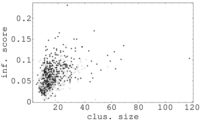
Figure 9: Resampling test for the clusters of data set from ref. McCue et al. (2001). Each filled black star is a cluster obtained by annealing the real data set, while each gray open star is a cluster obtained by annealing the randomized data set. Cluster sizes are shown horizontally, while their WM information scores $I$ are shown vertically.

Fig. 9 shows the results of the resampling test on the results of data from ref. McCue et al. (2001). The filled black stars show the clusters that were obtained at the end of annealing for the real data set. The number of sequences in each cluster is shown on the horizontal axis, while each cluster’s WM score $I$ is shown on the vertical axis. Similarly, the gray open stars show the clusters obtained by the annealing of the randomized data set. We will call a cluster significant if there is no cluster of the same size and with higher information score in the randomized data set. Of course, it would be better to perform many resampling runs and estimate more precisely the probability of annealing random data producing a cluster with information score larger than $I$ at each possible cluster size. This is computationally rather intensive. Since we are assessing significance of clusters within a Bayesian framework, we provide the data in Fig. 9 as a guideline for comparison with significance tests that are more commonly used. Under our definition of significance for the resampling test we find $88$ significant clusters, which are mostly the same clusters as deemed significant by our Bayesian procedure.

Appendix F Operations on the Data Sets

In this section we briefly describe the data sets that were used in our studies and describe in more detail the operations that we performed on these data sets before clustering them using PROCSE.

The data set from ref. McCue et al. (2001) contains multiple alignments of putative binding sites from a number of related proteobacteria and was collected in the following way. For each E. coli gene, orthologous genes were collected from the species Actinobacillus actinomycetemcomitans, Haemophilus influenzae, Pseudomonas aeruginosa, Shewanella putrefaciens, Salmonella typhi, Thiobacillus ferrooxidans, Vibrio cholerae, and Yersinia pestis. A modified version of the Gibbs sampler algorithm Lawrence et al. (1993) is then used to find common motifs in the upstream regions of these orthologues. The resulting alignments of putative binding sites contain between 1 and 16 sequence segments with lengths of $15$-$25$ bases. We will interpret these alignments as collections of binding sites for the same TF.

The data set from ref. Rajewsky et al. (2002) contains similar alignments of putative binding sites for a single TF but was obtained in a somewhat different manner. Again, sets of orthologous genes were collected for each E. coli gene from the species Klebsiella pneumoniae, S. typhi, V. cholerae, and Y. pestis. Instead of looking for similar sequence motifs in the upstream regions, ref. Rajewsky et al. (2002) aligned the upstream regions and found sequence segments that are more conserved than sequences downstream of orthologous genes. The resulting alignments differ from those of ref. McCue et al. (2001) in two respects. First, there are more stringent constraints on the selection of conserved sequence segments. Second, since the number of species used is smaller, the number of sequences in the alignment per upstream region is generally smaller.

F.1 Operations on the Data Set from McCue et al. (2001)

Ref. McCue et al. (2001) have annotated alignments in their data set for which the E. coli site overlaps either a known site, or a known repetitive element. We have removed all such alignments from our data set, since for this data set, we are interested in clustering new putative binding sites. We then ordered all the remaining alignments by their MAP value. The MAP value is a quality measure given to the alignments by ref. McCue et al. (2001). We then went through the ordered list of alignments and removed alignments whose centers are less than $6$ bases away from centers of previous alignments in the list. This is to avoid the possibility of the algorithm aligning the same mini-WM twice in a cluster. Overlaps are only checked for the E. coli members of the alignment. We then took the top 2,000 of the remaining alignments as our data set.

After that we symmetrically extended all alignments from their original length (between 15 and 25 bases) to length 32. To do so we had to “pad” bases to the alignments from the genomes. Some of the genomes used by ref. McCue et al. (2001) are not yet completed and some cases occurred in which the bases could not be padded because the sequence is not available. In those rare cases, we added random bases to replace the missing bases. As pointed out in the paper, we would like to consider the sequences in the resulting alignment as independent samples from a WM describing the TF. However, some of the species are probably too closely related evolutionary to warrant this assumption of independence. That is, some of the bases in the alignment are conserved not because of selectional constraints but because they simply haven’t mutated yet since the species diverged. Ideally we would deal with these evolutionary relationships directly, reconstructing the phylogenetic tree of the species involved, and inferring which bases in the alignment have been retained by selection. However, this is an altogether separate inference problem and we opted for a simple circumvention of this problem. We replaced the sequences from the most closely related species by their consensus. That is, we replaced triplets of sequences from E. coli, S. typhi, and Y. pestis with their consensus, and replaced sequences from the pair H. influenzae and A. actinomycetemcomitans with their consensus as well. We deem all other species to be sufficiently separated evolutionary such that we can assume their sequences to be independent samples of a WM. There are two more technical details to mention regarding this procedure. First, there may not be a majority base among the sequences. In those cases we select one of the bases among the triplet (or pair) of sequences at random. The second problem arises because the alignments of ref. McCue et al. (2001) may contain more than one sequence segment from the same upstream region, i.e. from the same genome. Thus, if we have two segments from S. typhi and two from E. coli occurring in the same alignment, we have to decide how to pair these before taking their consensus. We do this by picking the pairing that maximizes the number of conserved bases between the paired segments. These operations now give us the mini-WMs on which the PROCSE algorithm operates.

F.2 Operation on the data set from Rajewsky et al. (2002)

The operations on the data set from ref. Rajewsky et al. (2002) are largely the same as those described in the previous section. We used the set of predicted E. coli binding sites from Rajewsky et al. (2002) and the corresponding local alignments to construct a mini-WM of length $32$ for each putative binding site $x$. In case the length $l(x)$ was $<32$, we padded additional bases to the left and to the right using the most significantly conserved E. coli base $b$ as an anchor. Similarly, if $l(x)>32$, sites were clipped off. The sequences for E. coli, K. pneumoniae, and S. typhi were replaced by their consensus. Each mini-WM was scored by the significance score for $b$ Rajewsky et al. (2002) and ordered accordingly. Alignments that overlapped an alignment with higher score with $27$ or more bases were removed. In contrast to the algorithm employed in McCue et al. (2001), the selection of sites in this data set was not optimized to maximize the inclusion of known binding sites or to favor reverse complement symmetry of the sites. For this reason, we did not remove sites that overlap known binding sites (or known repetitive elements) from this set. By comparing the results obtained with this data set and those obtained with the data set from McCue et al. (2001), we may (to some extent) assess the effect on the discovery of new vs. known regulons of the removal/inclusion of known sites.

F.3 Processing of the data set from Robison et al. (1998)

The data set of known TF binding sites from Church’s lab Robison et al. (1998) contains a total of $997$ sites. In order to create a test set for our algorithm we filtered this set in several ways. First we removed all $\sigma$-factor binding sites. There are several reasons for removing these sites. First of all, $\sigma$-$70$ sites are ubiquitous in the genome, whereas we are interested in finding regulons (sites and their TFs) that specifically regulate (relatively) small sets of genes. Second, there are regulatory sites that overlap $\sigma$-sites, and since in our algorithm any piece of genome can only occur in one cluster at a time, these sites would alternatively cluster with the regulon of interest and with the rest of the $\sigma$-sites at other times. The presence of the $\sigma$-sites would thus negatively effect the inference of other (smaller) regulons. Finally, the primary data set McCue et al. (2001) looked for reverse complement symmetry in the binding sites, thus disfavoring the inclusion of $\sigma$-sites in their data set. Thus, removing the $\sigma$-sites from the tes -set makes it also more comparable with the data set from ref. McCue et al. (2001).

After removing $\sigma$-sites and sites that overlap each other by more than $27$ bases there are $397$ unique TF binding sites in this data set.

F.4 Preparation of TF mini-WMs from Data Set Robison et al. (1998)

When we cluster the new putative binding sites we want to separate clusters of sites that correspond to TFs for which some binding sites are already known from clusters of sites that form entirely new putative regulons. To this end we took all the known binding sites from the collection from Robison et al. (1998) and divided them into groups according to their annotation. That is, all sites that are annotated as binding sites for the same TF form a group. We then aligned these groups of sites into alignments of all known sites for each TF. The multiple alignment is performed by running a hierarchical clustering with our scoring function. That is, we first put all known sites for a TF into separate clusters and then find the pair that, when fused, leads to the largest increase in the score $P(D|C)$ of the partition. We repeat this procedure (i.e. at the second step either a third sequence is added to the pair or another pair is fused) until a single cluster is left. At each step the alignment is maximized over all possible ways of shifting the sites with respect to each other and both strands. Thus, we sometimes have to pad bases from the genome to “complete” the alignment. At the end, the length $32$ window with the highest information score is taken from the alignment. The mini-WM so obtained represents all known sites for a particular TF. We constructed $56$ different mini-WMs in this way from data set Robison et al. (1998). There are only $53$ TFs represented in this data set, but three of them (metJ, argR, and phoB) have two different types of sites, which we aligned separately.

We added these $56$ mini-WMs to both data sets. The idea is that if additional binding sites for any one of these TFs occur in our data set, then these sites will tend to cluster with one of the $56$ mini-WMs that we have just described. When we collect the significant clusters at the end of the run, we separate them into two sets: those that contain at least one of the 56 mini-WMs constructed from Robison et al. (1998) and those that do not. The former clusters contain new putative sites for known regulons, while the latter contain new predicted regulons.

Appendix G Results of Clustering Known Binding Sites

Table 2 shows results from clustering the set of $397$ sites from ref. Robison et al. (1998). We performed several different tests of our algorithm with this data.

fac.	size	int.	size	num. site	int.	size	num. site	int.
arcA	12	2-5	20/15	3/3	1-11/1-11	24	4	1-14
argR2	7	5-7	21/24	7/7	8-20/11-21	26	5	1-11
argR	17	8-14	22/22	10/12	12-21/11-21	-	-	-
crp	41	13-27	22/29	19/20	2-16/7-21	39	19	7-28
dnaA	8	3-6	7/8	6/6	3-7/3-7	-	-	-
fadR	7	4-7	12/9	7/7	3-10/3-8	11	4	1-8
fis	11	2-3	20/15	4/4	1-11/1-11	-	-	-
fnr	12	7-9	11/11	9/9	7-10/7-10	25	6	17-23
fruR	11	8-11	17/13	11/10	8-13/7-12	15	7	1-6
fur	8	5-6	21/24	5/6	8-20/11-21	28	6	19-24
galR	6	3-6	6/14	5/6	3-6/3-8	9	2	1-4
hipB	4	3-4	8/14	3/4	2-5/4-13	-	-	-
ihf	18	3-5	22/22	5/4	12-21/11-21	27	5	5-15
lexA	19	18-19	24/24	19/19	19-23/19-23	28	18	19-24
lrp	14	2-4	-/-	-/-	-/-	-	-	-
malT	10	2-6	9/8	7/6	1-6/1-6	-	-	-
metJ(3)	15	13-15	17/15	14/13	14-17/13-15	17	14	13-16
narL	9	2-6	10/14	5/6	1-5/4-13	-	-	-
ntrC	5	5-5	9/10	5/5	5-7/5-8	18	14	9-14
phoB	9	2-4	9/13	3/4	1-7/1-8	11	4	1-8
purR	16	13-15	15/17	14/16	13-15/13-16	23	13	16-20
trpR	3	2-3	8/-	3/-	1-5/-	-	-	-
tus	5	4-5	11/8	5/5	5-8/5-7	12	5	3-6
tyrR	16	5-11	15/21	9/8	2-10/1-13	-	-	-

Table 2: Clustering of the $397$ sites from ref. Robison et al. (1998). Column $1$ shows the TF name, column $2$ shows the number of sites in the data set annotated as binding sites for that TF (according to ref. Robison et al. (1998)), column 3 shows the the $90$% probability interval for the number of coclustering sites for this TF. Only those TFs are shown for which the lower bound of the $90$% probability interval is $2$ or higher. We performed two annealing runs of this data set to find the ML partition. For each TF, we found the cluster in this partition with the largest number of sites for that TF. The clusters shown in columns $4$-$6$ resulted from two simulated annealing runs, with the “size” and “int” defined as before. Column 5 shows how many of the sites in column 4 were annotated for the TF. For example, columns $4$-$6$ for the TF dnaA show that at the end of the two annealing runs there were clusters of sizes $7$ and $8$, respectively that both contained $6$ of the $8$ known dnaA binding sites, and with $90$% probability between $3$ and $7$ members of these clusters co-cluster. Finally, columns $7$-$9$ show the same statistics when the annealing is done on a larger data set that contains both the $397$ sites of ref. Robison et al. (1998) as well as the top $2,000$ E. coli sites from ref. McCue et al. (2001).

First of all, one may test how well the known binding sites cluster according to their annotation. That is, do sites annotated to be binding sites for the same TF $X$ significantly cluster with each other? To answer this question, we performed Monte Carlo sampling of the probability distribution $P(C|D)$ for this data set. At each time step of the Monte Carlo random walk, we measure how many sites of each TF “cocluster”. This is defined as follows: At any particular time step of the Monte Carlo walk, the sites that are annotated for TF $X$ will be distributed in some way among the clusters that are present at that time during the random walk. For instance, if TF $X$ has $10$ binding sites in the data, $6$ of those may sit in one cluster, $2$ others may sit in another cluster together with some sites of different annotation, and the last $2$ may each sit in some cluster that is dominated by sites of other annotation. For such a partition, we would say that $6$ of the $10$ sites for TF $X$ cocluster. By calculating how many sites cocluster at each time step, we measure, for each TF, the distribution $p(k)$ that $k$ of its sites will cocluster at any point in time. These distributions may be summarized in various ways, but we chose to find the shortest length interval $[k_{\rm min},k_{\rm max}]$ such that at least $90$% of the time between $k_{\rm min}$ and $k_{\rm max}$ sites cocluster, i.e. $\sum_{k=k_{\rm min}}^{k_{\max}}p(k)>0.9$. We will consider the sites of a TF $X$ to cluster “significantly” if $k_{\rm min}>1$ for its distribution $p(k)$. Of the $53$ TFs represented in the data set, there are 24 that cluster significantly. These are shown in the rows of Table 2. The first column shows the name of the TF, the second column shows the total number of sites for that TF contained in the $397$-site data set, and the third column shows the interval $[k_{\rm min},k_{\rm max}]$. The fifth row, for instance, shows that the TF dnaA has a total of $8$ sites in the data set, and that at least $90$% of the time between $3$ and $6$ of these sites cocluster.

As mentioned before, $24$ of the $53$ TFs cluster significantly. One might call this an overall “false negative” rate of $55$%. All the TFs that cluster significantly (with the exception of trpR) have more than three binding sites in the data set. There are $22$ TFs that have $3$ or less sites in the data. Therefore, it is clear that it is mostly TFs with a small number of samples in the data that do not cluster significantly. In other words, there is a false negative rate of less than $23$% for TFs with more than three sites in the data set. Table 3 shows the TFs whose sites did not cluster significantly. Note that some of these sites (such as cpxR, flhCD, glpR, metR, modE, nagC, ompR) do cluster significantly better than sets of random sequences would, but did not pass our significance threshold. That is, we could have changed the significance thresholds such that for this particular data set the number of false negatives would be further decreased. Still, it is quite clear that the sites for a TF like soxS do not cluster at all. The variability among the $8$ soxS sites is so large that one might wonder if a WM model is appropriate at all for TFs like this.

In this first test, we used the annotation of the sites to measure to what extent sites with equal annotation cluster together. Summarizing, we found significant clustering for slightly less than half of the TFs, and for over $75$% of the TFs that have more than 3 sites in the data set. After this, we wanted to test to what extent our annealing approach will be able to identify the “correct” clusters. That is, we wanted to compare the ML clusters that result from annealing with the annotation of the sites. We performed two annealing runs to identify a ML partition. We tested the significance of the ML clusters obtained by annealing by performing two sampling runs. Again we measure the coclustering distribution $p(k)$ for each cluster and consider a cluster significant if the $90$% probability interval $[k_{\rm min},k_{\rm max}]$ has $k_{\rm min}>1$.

fac.	size	int.
ada	2	1-1
araC	4	1-2
carP	2	1-1
cpxR	6	1-3
cspA	4	1-2
cynR	2	1-1
cysB	3	1-1
cytR	5	1-2
deoR	1	1-1
farR	3	1-2
fhlA	3	1-1
flhCD	3	1-3
gcvA	4	1-2
glpR	7	1-3
hns	3	1-1
hu	1	1-1
iclR	1	1-1
ilvY	2	1-1
lacI	1	1-1
marR	2	1-2
metR	7	1-4
modE	3	1-3
nagC	6	1-3
ompR	8	1-3
oxyR	3	1-2
pdhR	2	1-1
rhaS	2	1-1
soxS	8	1-2
torR	1	1-3

Table 3: TFs from data set Robison et al. (1998) whose sites did not cluster significantly. First column is TF name, second is the total number of binding sites for that TF in the data, and the third column is the $90$% probability interval $[k_{\rm min},k_{\rm max}]$ of its coclustering distribution $p(k)$.

In order to compare these clusters with the annotation, we had to identify, for each TF, which of the ML clusters “corresponds” best to the cluster of binding sites of the TF. We do this by simply finding the ML cluster that contains the largest number of sites for the TF. That is, the $10$ sites of TF $X$ may be spread over $4$ clusters in the ML partition, with $5$ sites in one cluster, $3$ in another, and $2$ more in a third and fourth cluster. We would then identify the ML cluster containing the $5$ sites as the cluster “corresponding” to TF $X$.

These clusters are shown in columns $4$ through $6$ of table 2. The column entries are best explained by example. Focus, for instance, on the line for TF narL. In the first annealing run, there was a ML cluster that contained $5$ of the $9$ narL sites. This cluster had a total size of $10$ sequences (that is, apart from the $5$ narL members, $5$ members had different annotations). Under sampling, between $1$ and $5$ sites of this cluster cocluster $90$% of the time. (Note that this means: between $1$ and $5$ of the full set of $10$ sites.) In the second annealing run, there was a ML cluster of size $14$ that contains $6$ of the $9$ narL sites. Between $4$ and $13$ members of this cluster cocluster $90$% of the time. To give an example of a TF for which essentially the same cluster was found in both annealing runs, focus on the lexA line. In both runs there was a cluster of size $24$ that contained all $19$ of the known lexA sites (and $5$ sites with a different annotation). During sampling, between $19$ and $23$ members of this cluster cocluster (being one of the most stable clusters in the set).

In general, one can see that there is good agreement between the annotation and the clusters inferred by annealing. Looking in more detail at some of the annealed clusters, we note that narL and narP sites cluster together, as do fur and argR2 sites. The ihf sequences sit mostly in the tail of the argR cluster and the fis sequences occupy the tail of the arcA cluster. The many crp sites sit distributed over two clusters (with only the largest represented in the table).

This test also allows us to assess the amount of false positives that our algorithm produces. At the end of the annealing there were $30$ and $29$ clusters in the two respective runs. After sampling, it turns out that $20$ of the $30$ we deemed significant using our cut-offs, and $16$ of the $29$ in the other run. None of these clusters are false positives. That is, our false positive rate is $0$ for this particular test set.

Finally, one may think that the annealing had not really found the ML clustering (or something close to that), but had gotten stuck in some local optimum, and that if we had had more time, and cooled slower, we may have found clusterings with better score that correspond even better to the known annotation. This is unlikely. One can easily calculate what the probability $P(C|D)$ is of the partition in which all sites are clustered according to their annotation. We find that this probability is substantially lower than the probability of the partitions that annealing finds. We believe that this has two main reasons. First, we believe that some of the sites are mis-annotated. Some sites of annotation $X$ consistently cluster with sites of some other annotation $Y$. Second, for some TFs (such as lrp, fis, ihf and soxS mentioned above) it seems that the WM representation of the sites is unsatisfactory. Their WM scores are extremely low: when we, for instance, run the clustering algorithm on only the fis sites, the algorithm prefers partitions in which these sites are not partitioned into a single cluster at all! Possibly, these TFs recognize something else than a sequence motif that can be represented by a WM.

References

- McCue et al. (2001) L. A. McCue, W. Thompson, C. S. Carmack, M. P. Ryan, J. S. Liu, V. Derbyshire, and C. E. Lawrence, Nucleic Acids Research 29, 774 (2001).
- Rajewsky et al. (2002) N. Rajewsky, N. D. Socci, M. Zapotocky, and E. D. Siggia, Genome Research 12, 298 (2002).
- Robison et al. (1998) K. Robison, A. M. McGuire, and G. M. Church, Journal of Molecular Biology 284, 241 (1998), http://arep.med.harvard.edu/dpinteract.
- Salgado et al. (2000a) H. Salgado, A. Santos-Zavaleta, S. Gama-Castro, D. Millan-Zarate, F. Blattner, and J. Collado-Vides, Nucl. Acids Res. 28, 65 (2000a).
- Salgado et al. (2000b) H. Salgado, G. Moreno-Hagelsieb, T. Smith, and J. Collado-Vides, Proc Natl. Acad. Sci USA 97, 6652 (2000b).
- Stormo and Hartzell (1989) G. D. Stormo and G. W. Hartzell, Proc. Natl. Acad. Sci. U.S.A. 86, 1183 (1989).
- Lawrence et al. (1993) C. E. Lawrence, S. F. Altschul, M. S. Boguski, J. S. Liu, A. F. Neuwald, and J. C. Wootton, Science 262, 208 (1993).
- Bailey and Elkan (1994) T. Bailey and C. Elkan, Proceedings ISMB’94 2, 28 (1994).
- Bussemaker et al. (2000) H. J. Bussemaker, H. Li, and E. D. Siggia, Proc. Natl. Acad. Sci. U.S.A. 97, 10096 (2000).
- Hardison et al. (1997) R. Hardison, J. Oeltjen, and W. Miller, Genome Res. 10, 959 (1997).
- Gelfand et al. (2000) M. Gelfand, E. Koonin, and A. Mironov, Nucleic Acids Res. 28, 695 (2000).
- McGuire et al. (2000) A. M. McGuire, J. D. Hughes, and G. M. Church, Genome Res. 10, 744 (2000).
- Berg and von Hippel (1987) O. G. Berg and P. H. von Hippel, J. Mol. Biol. 193, 723 (1987).
- de Bruijn (1958) N. G. de Bruijn, Asymptotic Methods in Analysis (Dover Inc., 1958).
- Metropolis et al. (1953) N. Metropolis, A. W. Rosenbluth, M. N. Rosenbluth, A. H. Teller, and E. Teller, J. Chem. Phys 21, 1087 (1953).
- (16) website, all clusters can be found at http://www.physics.rockefeller.edu/erik/website_explanation.html.
- Begley et al. (1999) T. Begley, D. Downs, S. Ealick, F. McLafferty, and A. van Loon et. al., Arch. Microbiol. 171, 293 (1999).
- Miranda-Rios et al. (2001) J. Miranda-Rios, M. Navarro, and M. Soberón, Proceedings of the National Academy of Sciences 98, 9736 (2001).
- Bausch et al. (1998) C. Bausch, N. Peekhaus, C. Utz, T. Blais, E. Murray, T. Lowary, and T. Conway, Journal of Bacteriology 180, 3704 (1998).
- Peekhaus and Conway (1998a) N. Peekhaus and T. Conway, J. Bacteriol. 180, 3495 (1998a).
- Peekhaus and Conway (1998b) N. Peekhaus and T. Conway, J. Bacteriol. 180, 1777 (1998b).
- Neidhardt (1996) F. C. Neidhardt, ed., Escherichia coli and Salmonella Typhimurium. Cellular and molecular biology (ASM press, Washington D.C., 1996).
- Jacobson and Fuchs (1998) B. A. Jacobson and J. A. Fuchs, Molecular Microbiology 28, 1315 (1998).
- (24) Ecocyc, The ecocyc database, http://ecocyc.pangeasystems.com/.
- Jennings and Beacham (1990) M. Jennings and I. Beacham, J. Bacteriol. 172, 1491 (1990).
- Cheek and Broderick (2001) J. Cheek and J. Broderick, J. Biol. Inorg. Chem. 6, 209 (2001).
- van Nimwegen et al. (1999) E. van Nimwegen, J. P. Crutchfield, and M. Huynen, Proc. Natl. Acad. Sci. USA 96, 9716 (1999).
- Sengupta et al. (2002) A. M. Sengupta, M. Djordjevic, and B. I. Shraiman, Proc. Natl. Acad. Sci. USA 99, 2072 (2002).
- Jaynes (1983) E. T. Jaynes, Papers on probability, statistics, and statistical physics, vol. 158 of Synthese library (D. Reidel publishing company, Dordrecht Holland, 1983), r.D. Rosenkrantz, editor.