Floating Bodies of Equilibrium II
Franz Wegner, Institut für Theoretische Physik
Ruprecht-Karls-Universität Heidelberg
Philosophenweg 19, D-69120 Heidelberg
Email: wegner@tphys.uni-heidelberg.de
Abstract
In a previous paper (physics/0203061) ”Floating bodies of equilibrium I” I have shown that there exist two-dimensional non-circular cross-sections of bodies of homogeous density which can float in any orientation in water, which have a -fold rotation axis. For given they exist for different densities. However, this was found only in a Taylor-expansion in a parameter which described the distortion from the circular shape up to seventh order. Here a differential equation for the boundary curve is given and the non-circular boundary curve can be expressed in terms of an elliptic integral.
1 Introduction
Stanislaw Ulam asks in the Scottish Book [1] (problem 19), whether a sphere is the only solid of uniform density which will float in water in any position. In a recent paper[2] I considered the two-dimensional problem for . (The case has been solved by Auerbach [3]). I was able to obtain non-circular two-dimensional cross-sections of bodies which can flow in any orientation in water by a perturbative expansion around the circular solution. These cross-sections have a -fold rotation symmetry. In polar coordinates and the boundary-curve could be expanded in powers of a deformation-parameter
| (1) |
The coefficients were determined up to order . Although one has solutions for different densities , it turned out that was the same for all these densities.
Here a non-perturbative solution is given. It is shown that the boundary-curve obeys the differential equation
| (2) |
with . This equation can be integrated
| (3) | |||||
| (4) | |||||
and is thus given by an elliptic integral. With increasing the radius oscillates periodically between the largest and the smallest radii and , resp. The three constants , , and are determined by these extreme radii, and by the periodicity of the boundary. Since vanishes for the extrema of , one has
| (5) |
The periodicity is given by
| (6) |
The solution of the differential equation (2) expanded in powers of agrees completely with the expansion obtained in [2].
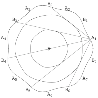
I explain now, how I arrived at this differential equation. Denote the two intersections of the water-line with the cross-section by and . From the general arguments given in [2] one knows, that the length of the water-line has to be independent of the orientation. (Here actually we will fix the orientation of the cross-section and rotate the water-line including the direction of the gravitational force.) The midpoint of the line moves in the direction of the chord as the water-line is rotated. Suppose the coordinates of the intersections are given by and . If the line moves by an infinitesimal amount , , then the condition, that the distance is fixed yields and the condition, that moves in the direction of yields . From both conditions we find, that under this change the same length of the perimeter disappears on one side below the water-line and appears on the other side above the water-line. Then , . Thus the angles between the tangents on the boundary and the water-line are the same on both ends.

In the following we will use these properties in two forms: (i) as line-condition, requiring, that the envelope of the water-lines is the loci of the midpoints , so that we obtain and by drawing tangents on the envelope and going a constant distance along the tangent in both directions to obtain and . (ii) as angle-condition, requiring, that moving and the same piece along the perimeter to and , the angles and between the tangents and the chord always obey . Both conditions are equivalent. From (i) follows (ii) and from (ii) follows (i).
In a next step consider the limit of large . Then will oscillate on a distance of order , which is small in comparison to itself. I assume, that then one can neglect the overall average curvature and one may find a periodic function of , which obeys the line-condition. Indeed assuming, that this holds for , that is on a distance of many periods, one can derive in this linear case a differential equation, which has to be obeyed by the function . This will be done in subsection 2.1. Expanding the solution in powers of is in agreement with the terms leading in which were found in eq. 86 of [2].
Unfortunately this procedure is not applicable for finite . Here I work with a new conjecture: Although for physical reasons the periodicity has to be an integer, one may try it with non-integer . If differs from an integer infinitesimally, then going around by the angle one arrives at the same function shifted however, in -direction by an infinitesimal angle . I conjecture that there is also a line between and belonging to angles differing by of constant small length , which obeys the line-condition. This condition yields a differential equation. For the linear case this is done in subsection 2.2. It is in agreement with that derived for large distance . For the circular case one obtains the differential equation in subsection 3.1, which is identical to eq. (2).
Finally it is shown in subsections 2.3 and 3.2, that the angle-condition holds for the curves described by the so obtained differential equations which are shifted by arbitrary distances in the linear case and by arbitrary angles in the circular case, resp. This last property can now also be used for two points and on the same curve, and thus shows that eq. (2) yields the boundaries for cross-sections with .
2 Linear Approximation
Consider now the above mentioned linear case. Let us start from the loci of the middle points of the chord , described by Cartesian coordinates . Then drawing the tangent on this curve and moving along the tangent by the distance in both directions one obtains the points and , which should lie on the same curve described by . Thus the functions and should obey
| (7) |
2.1 Large Distance
Assume now, that the functions are periodic with periodicity and , similarly for . Then for integer and has extrema at with odd . If we seek solutions for large , then we put with and small . We write
| (8) |
and obtain by expansion in and addition and subtraction of the equations
| (9) | |||||
| (10) |
Note that and . If is of order , then we realize from the second equation, that and thus is of order . The first equation yields, that is of order . We put . Furthermore we write and collect the leading terms of these two equations
| (11) |
where the argument of is and of is . From these two equations we obtain differential equations for and . Taking the derivative of the second equation and substituting into the first one yields
| (12) |
If we multiply this equation by , we can integrate it and obtain
| (13) |
In order to obtain a differential equation for we solve this equation for and differentiate it. This yields
| (14) |
and substituting the equation
| (15) |
or
| (16) |
which we will use in the form
| (17) |
with new integration constants and .
2.2 Infinitesimal distance
We perform now a similar calculation, but assume, that we can represent and similarly by , where now and are infinitesimally small. Thus we assume
| (18) |
It will turn out, that we need the expansion in to first order and in in third order. We obtain
| (19) | |||||
| (20) |
Differentiating the first equation yields
| (21) |
Equating both expressions and choosing yields
| (22) |
In the limit one has . With this substitution and multiplication by we may integrate this equation
| (23) |
Multiplication by allows a second integration which yields
| (24) |
Comparison with the equation obtained for large distances (17) shows agreement, if we change the notation for the constants. There is no linear term in eq.(17) like the term in eq.(24). The reason is, that in eq. (17) we required to vanish on the average. But of course a constant can be added to and , yielding such a linear term. Thus both procedures yield the same differential equation.
2.3 Arbitrary Distance
We show now the following theorem. Consider two curves and which are governed by eq. (17) with the same constants and , and point with Cartesian coordinates and with coordinates . If now the angle between the tangent in and equals the angle between the tangent in and , and , then this property will hold between any two points and , which are obtained by moving from and by the same arc in the same direction along the curves. Simultaneously the distance is constant.
In order to show this we first express the angles and . Let us denote the angles of the curves against the -axis by ,
| (25) | |||||
| (26) |
and the angle of against the -axis by ,
| (27) |
where is the distance .

Then we have , . The condition can now be expressed in various ways. From one obtains
| (28) |
which for reduces to
| (29) |
We show now, that
| (30) |
is independent of , if initially it vanishes, , and holds. For this purpose we calculate the derivative and show, that it vanishes, and thus, that remains 0. For this purpose we calculate the derivatives needed and indicate the derivative with respect to u by a dot,
| (31) | |||||
| (32) | |||||
| (33) |
We use generally for the derivatives of the angles
| (34) |
and obtain
| (35) |
and
| (36) |
We make now use of (29) and obtain
| (37) |
from which we conclude , provided
For one has . If the minus-sign applies, then vanishes for all and . In this case, however, , and we obtain . One can easily check, that for one obtains , so that holds also as we approach . Thus the theorem is proven.
Obviously instead of considering two curves, we may consider two points and on the same curve, which implies, that the midpoints of these chords are the envelope of these lines as we increase .
3 Circular Case
The point with polar coordinates lie on the tangent of the envelope through with polar coordinates a distance apart. Then we have
| (38) |
Denote the angle by . Then is related to the
slope of the tangent by and
. For we obtain
.
Thus we obtain
| (39) |
where the upper sign yields on the curve rotated by and the lower sign on the curve rotated by .

3.1 Infinitesimal angle
We expand both sides of eq. (39) up to order and and add and subtract the equations for both signs. Then we obtain
| (40) | |||||
| (41) | |||||
Now we differentiate eq. (40)
| (42) | |||||
and subtract eq. (41) from this derivative. The resulting equation contains terms proportional to and to . Thus we set proportional . In the limit the function approaches and similarly for the derivatives. Thus we have
| (43) | |||||
This differential equation can be integrated. One finds, that
| (44) |
with
| (45) | |||||
| (46) |
Thus and are constants. Elimination of yields the differential equation of the bounding curve quoted in the introduction, eq. (2).
| (47) |
with constants , , and .
3.2 Arbitrary angle
Now we consider the two curves rotated against each other by an arbitrary angle and perform similar calculations to those for the linear case.
We first express the angles
| (48) |
and show the following theorem: If the condition , that is
| (49) |
is fulfilled and and the points and move along their curves by the same arc to points and , then the condition remains fulfilled, that is for all these chords holds. Simultaneously the distance remains constant.
In order to show this we calculate . For this purpose we first list the sines and cosines of the angles
| (50) | |||||
| (51) | |||||
| (52) | |||||
| (53) | |||||
| (54) |
Their derivatives with respect to indicated by a dot are
| (55) | |||||
| (56) |
Performing the derivatives for and and using (55) one obtains
| (57) |
Thus we obtain using again eq. (34)
| (58) | |||||
| (59) |
Now we use in order to simplify the derivatives . First we evaluate which yields
| (60) |
Inserting this expression into eq.(57) yields
| (61) |
Further we determine the products from and , which yield
| (62) | |||||
| (63) |
For one obtains
| (64) | |||||
| (65) |
and thus
| (66) | |||||
| (67) |
from which one concludes provided
For one has and . If the minus sign applies, then and . In this case we are not allowed to divide by , which we did in our derivation. It turns out, however, that in this limit and one obtains
| (68) | |||||
| (69) | |||||
3.3 Application to the boundary
We may now apply the theorem to our original problem. In this problem the two curves are identical and constitute the boundary. Suppose we have now a curve obeying the differential equation (2) with integer . Then we have to look for points on this curve which have either the properties and or otherwise the properties and , eq. (68). We will now show, that there are at least solutions, which obey the second condition. For this purpose we divide the curve into pieces , … in which decreases from to as increases and into pieces , … , where increases from to . We now look for solutions and , where is in and in . Thus we have to find a solution of (68). We realize, that with the exception of the first term in (68) vanishes for and , since , because at these extrema.
On the other hand we can evaluate for these extrema
| (70) | |||||
| (71) |
The denominator of the integral (4) vanishes only at the extreme points and . If we express and in terms of , , and , then
Thus , and therefor the factors and in the expressions for are positive. Therefore one has and . Therefore changes sign between and . Since is a continuous function of , there must be a zero in between. This argument holds for all pieces with the exception of those adjacent to . (For those adjacent may become 0. In this limit one finds .) Therefore we have at least solutions, which is in agreement with those found in [2]. We leave aside the question, whether for sufficiently large ratios more solutions appear and whether there are other solutions for . We finally mention that in the near-circular case the periodicity is related to by , where is some intermediate radius.
4 Conclusion
We have given a closed representation of the boundaries of logs floating in any direction with in terms of a differential equation which can be solved by an elliptic integral. The differential equation could be obtained, since points of two of these curves rotated against each other can be connected by chords so that by progressing on the two curves by the same length of the perimeter the length of the chord does not change. Using that this holds also for two curves rotated against each other by an infinitesimal angle connected by a chord of infinitesimal length the differential equation could be derived. The differential equation of the linear analogue of this curve has also been given.
References
- [1] R.D. Mauldin (ed.), The Scottish Book, Birkhäuser Boston 1981
- [2] F. Wegner, Floating Bodies of Equilibrium I, e-Print archive physics/0203061
- [3] H. Auerbach, Sur un probleme de M. Ulam concernant l’equilibre des corps flottant, Studia Math. 7 (1938) 121-142