An Accurate, Simplified Model of Intrabeam Scattering

Abstract

Beginning with the general Bjorken-Mtingwa solution for intrabeam scattering (IBS) we derive an accurate, greatly simplified model of IBS, valid for high energy beams in normal storage ring lattices. In addition, we show that, under the same conditions, a modified version of Piwinski’s IBS formulation (where $\eta^{2}_{x,y}/\beta_{x,y}$ has been replaced by ${\cal H}_{x,y}$) asymptotically approaches the result of Bjorken-Mtingwa.

INTRODUCTION

Intrabeam scattering (IBS), an effect that tends to increase the beam emittance, is important in hadronicBhat et al. (1999) and heavy ionFischer et al. (2001) circular machines, as well as in low emittance electron storage ringsBane et al. . In the former type of machines it results in emittances that continually increase with time; in the latter type, in steady-state emittances that are larger than those given by quantum excitation/synchrotron radiation alone.

The theory of intrabeam scattering for accelerators was first developed by PiwinskiPiwinski (1974), a result that was extended by MartiniMartini (1984), to give a formulation that we call here the standard Piwinski (P) methodPiwinski (1999); this was followed by the equally detailed Bjorken and Mtingwa (B-M) resultBjorken and Mtingwa (1983). Both approaches solve the local, two-particle Coulomb scattering problem for (six-dimensional) Gaussian, uncoupled beams, but the two results appear to be different; of the two, the B-M result is thought to be the more generalPiwinski .

For both the P and the B-M methods solving for the IBS growth rates is time consuming, involving, at each time (or iteration) step, a numerical integration at every lattice element. Therefore, simpler, more approximate formulations of IBS have been developed over the years: there are approximate solutions of ParzenParzen (1987), Le DuffDuff (1989), RaubenheimerRaubenheimer (1991), and WeiWei (1993). In the present report we derive—starting with the general B-M formalism—another approximation, one accurate and valid for high energy beams in normal storage ring lattices. We, in addition, demonstrate that under these same conditions a modified version of Piwinski’s IBS formulation asymptotically becomes equal to this result.

HIGH ENERGY APPROXIMATION TO BJORKEN-MTINGWA

The General B-M SolutionBjorken and Mtingwa (1983)

Let us consider first machines with bunched beams that are uncoupled and have vertical dispersion due to e.g. orbit errors. Let the intrabeam scattering growth rates be defined as

$${1\over T_{p}}={1\over\sigma_{p}}{d\sigma_{p}\over dt}\ ,\quad{1\over T_{x}}={1\over\epsilon_{x}^{1/2}}{d\epsilon_{x}^{1/2}\over dt}\ ,\quad{1\over T_{y}}={1\over\epsilon_{y}^{1/2}}{d\epsilon_{y}^{1/2}\over dt}\ ,$$ (1)

with $\sigma_{p}$ the relative energy spread, $\epsilon_{x}$ the horizontal emittance, and $\epsilon_{y}$ the vertical emittance. The growth rates according to Bjorken-Mtingwa (including a $\sqrt{2}$ correction factorKubo and Oide (2001), and including vertical dispersion) are

$${1\over T_{i}}\ =\ 4\pi A({\rm log})\bigg{<}\int_{0}^{\infty}{d\lambda\,\lambda^{1/2}\over[{\rm det}(L+\lambda I)]^{1/2}}\bigg{\{}$$

$$TrL^{(i)}Tr\left({1\over L+\lambda I}\right)-\ 3TrL^{(i)}\left({1\over L+\lambda I}\right)\bigg{\}}\bigg{>}\quad\ \$$ (2)

where $i$ represents $p$, $x$, or $y$;

$$A={r_{0}^{2}cN\over 64\pi^{2}\bar{\beta}^{3}\gamma^{4}\epsilon_{x}\epsilon_{y}\sigma_{s}\sigma_{p}}\quad,$$ (3)

with $r_{0}=2.82\times 10^{-15}$ m, the classical electron radius, $c$ the speed of light, $N$ the bunch population, $\bar{\beta}$ the velocity over $c$, $\gamma$ the Lorentz energy factor, and $\sigma_{s}$ the bunch length; $({\rm log})$ represents the Coulomb log factor, $\langle\rangle$ means that the enclosed quantities, combinations of beam parameters and lattice properties, are averaged around the entire ring; ${\rm det}$ and $Tr$ signify, respectively, the determinant and the trace of a matrix, and $I$ is the unit matrix. Auxiliary matrices are defined as

$$L=L^{(p)}+L^{(x)}+L^{(y)}\quad,$$ (4)

$$L^{(p)}={\gamma^{2}\over\sigma_{p}^{2}}\left(\begin{array}[]{ccc}0&0&0\\ 0&1&0\\ 0&0&0\end{array}\right)\quad,$$ (5)

$$L^{(x)}={\beta_{x}\over\epsilon_{x}}\left(\begin{array}[]{ccc}1&-\gamma\phi_{x}&0\\ -\gamma\phi_{x}&{\gamma^{2}{\cal H}_{x}/\beta_{x}}&0\\ 0&0&0\end{array}\right)\quad,$$ (6)

$$L^{(y)}={\beta_{y}\over\epsilon_{y}}\left(\begin{array}[]{ccc}0&0&0\\ 0&{\gamma^{2}{\cal H}_{y}/\beta_{y}}&-\gamma\phi_{y}\\ 0&-\gamma\phi_{y}&1\end{array}\right)\quad.$$ (7)

The dispersion invariant is ${\cal H}=[\eta^{2}+(\beta\eta^{\prime}-{1\over 2}\beta^{\prime}\eta)^{2}]/\beta$, and $\phi=\eta^{\prime}-{1\over 2}\beta^{\prime}\eta/\beta$, where $\beta$ and $\eta$ are the beta and dispersion lattice functions.

For unbunched beams $\sigma_{s}$ in Eq. 2 is replaced by $C/(2\sqrt{2\pi})$, with $C$ the circumference of the machine.

The Bjorken-Mtingwa Solution at High Energies

Let us first consider $1/T_{p}$ as given by Eq. 2. We first notice that, for normal storage ring lattices (where $\langle{\cal H}_{x,y}/\beta_{x,y}\rangle\ll 1$), the off-diagonal elements in $L$, $-\gamma\phi$, are small and can be set to zero. Then all matrices are diagonal. Let us also limit consideration to high energies, i.e. let us assume $a$,$b\ll 1$, with

$$a={\sigma_{H}\over\gamma}\sqrt{\beta_{x}\over\epsilon_{x}}\quad,\quad\quad b={\sigma_{H}\over\gamma}\sqrt{\beta_{y}\over\epsilon_{y}}\quad,$$ (8)

with

$${1\over\sigma_{H}^{2}}={1\over\sigma_{p}^{2}}+{{\cal H}_{x}\over\epsilon_{x}}+{{\cal H}_{y}\over\epsilon_{y}}\quad.$$ (9)

Note that if $a$,$b\ll 1$, then the beam is cooler longitudinally than transversely. If we consider, for example, KEK’s ATF, a 1.4 GeV, low emittance electron damping ring, $\epsilon_{y}/\epsilon_{x}\sim 0.01$, $a\sim 0.01$, $b\sim 0.1$Bane et al. .

If the high energy conditions are met then the 2nd term in the braces of Eq. 2 is small compared to the first term, and can be dropped. Now note that $L_{2,2}$ can be written as $\gamma^{2}/\sigma_{H}^{2}$. For high energy beams a factor in the denominator of the integrand of Eq. 2, $\sqrt{\gamma^{2}/\sigma_{H}^{2}+\lambda}$, can be approximated by $\gamma/\sigma_{H}$; also, the (2,2) contribution to $Tr[(L+\lambda I)^{-1}]$ becomes small, and can be set to 0. Finally, the first of Eqs. 2 becomes

$${1\over T_{p}}\approx{r_{0}^{2}cN({\rm log})\over 32\gamma^{3}\epsilon_{x}^{3/4}\epsilon_{y}^{3/4}\sigma_{s}\sigma_{p}^{3}}\left<\sigma_{H}\,g(a/b)\,\left({\beta_{x}\beta_{y}}\right)^{-1/4}\right>\ ,$$ (10)

with

$$g(\alpha) = {4\sqrt{\alpha}\over\pi}\int_{0}^{\infty}{dy\,y^{2}\over\sqrt{(1+y^{2})(\alpha^{2}+y^{2})}}\ \times$$ (11)

$$\times\ \left({1\over 1+y^{2}}+{1\over\alpha^{2}+y^{2}}\right)\quad.$$

A plot of $g(\alpha)$ over the interval [$0<\alpha<1$] is given in Fig. 1; to obtain the results for $\alpha>1$, note that $g(\alpha)=g(1/\alpha)$. A fit to $g$,

$$g(\alpha)\approx 2\alpha^{(0.021-0.044\ln\alpha)}\quad\quad[{\rm for}\ 0.01<\alpha<1]\quad,$$ (12)

is given by the dashes in Fig. 1. The fit has a maximum error of 1.5% over [$0.02\leq\alpha\leq 1$].

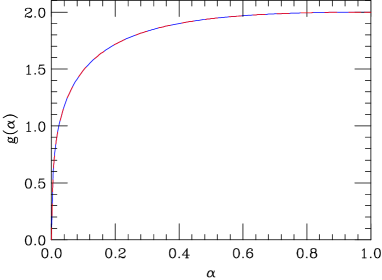
Figure 1: The auxiliary function $g(\alpha)$ (solid curve) and an analytical approximation, $g=2\alpha^{(0.021-0.044\ln\alpha)}$ (dashes).

Similarly, beginning with the 2nd and 3rd of Eqs. 2, we obtain

$${1\over T_{x,y}}\approx{\sigma_{p}^{2}\langle{\cal H}_{x,y}\rangle\over\epsilon_{x,y}}{1\over T_{p}}\quad.$$ (13)

Our approximate IBS solution is Eqs. 10,13. Note that Parzen’s high energy formula is a similar, though more approximate, result to that given hereParzen (1987); and Raubenheimer’s approximation is formulas similar, though less accurate, than Eq. 10 and identical to Eqs. 13Raubenheimer (1991).

Note that the beam properties in Eqs. 10,13, need to be the self-consistent values. Thus, for example, to find the steady-state growth rates in electron machines, iteration will be required. Note also that these equations assume that the zero-current vertical emittance is due mainly to vertical dispersion caused by orbit errors; if it is due mainly to (weak) $x$-$y$ coupling we let ${\cal H}_{y}=0$, drop the $1/T_{y}$ equation, and simply let $\epsilon_{y}=\kappa\epsilon_{x}$, with $\kappa$ the coupling factorBane et al. .

COMPARISON TO THE PIWINSKI SOLUTION

The Standard Piwinski SolutionPiwinski (1999)

The standard Piwinski solution is

$${1\over T_{p}} = A\left<{\sigma_{h}^{2}\over\sigma_{p}^{2}}f(\tilde{a},\tilde{b},q)\right>$$

$${1\over T_{x}} = A\left<f({1\over\tilde{a}},{\tilde{b}\over\tilde{a}},{q\over\tilde{a}})+{\eta_{x}^{2}\sigma_{h}^{2}\over\beta_{x}\epsilon_{x}}f(\tilde{a},\tilde{b},q)\right>$$

$${1\over T_{y}} = A\left<f({1\over\tilde{b}},{\tilde{a}\over\tilde{b}},{q\over\tilde{b}})+{\eta_{y}^{2}\sigma_{h}^{2}\over\beta_{y}\epsilon_{y}}f(\tilde{a},\tilde{b},q)\right>\ .$$ (14)

Parameters are:

$${1\over\sigma_{h}^{2}}={1\over\sigma_{p}^{2}}+{\eta_{x}^{2}\over\beta_{x}\epsilon_{x}}+{\eta_{y}^{2}\over\beta_{y}\epsilon_{y}}\quad,$$ (15)

$$\tilde{a}={\sigma_{h}\over\gamma}\sqrt{\beta_{x}\over\epsilon_{x}},\quad\tilde{b}={\sigma_{h}\over\gamma}\sqrt{\beta_{y}\over\epsilon_{y}},\quad q=\sigma_{h}\beta\sqrt{{2d\over r_{0}}}\quad,$$ (16)

The function $f$ is given by:

$$f(\tilde{a},\tilde{b},q) = 8\pi\int_{0}^{1}du\,{1-3u^{2}\over PQ}\ \times$$ (17)

$$\times \left\{2\ln\left[{q\over 2}\left({1\over P}+{1\over Q}\right)\right]-0.577\ldots\right\}$$

where

$$P^{2}=\tilde{a}^{2}+(1-\tilde{a}^{2})u^{2},\quad\quad Q^{2}=\tilde{b}^{2}+(1-\tilde{b}^{2})u^{2}\ .$$ (18)

The parameter $d$ functions as a maximum impact parameter, and is normally taken as the vertical beam size.

Comparison of Modified Piwinski to the B-M Solution at High Energies

To compare with the B-M solution, let us consider a slightly changed version of Piwinski that we call the modified Piwinski solution. It is the standard version of Piwinski, but with $\eta^{2}/\beta$ replaced by ${\cal H}$ (i.e. $\tilde{a}$, $\tilde{b}$, $\sigma_{h}$, become $a$, $b$, $\sigma_{H}$, respectively). Let us also assume high energy beams, i.e. let $a$,$b\ll 1$.

Let us sketch the derivation. First, notice that in the integral of the auxiliary function $f$ (Eq. 17): the $-0.577$ can be replaced by 0; the $-3u^{2}$ in the numerator can be set to 0; $P$ ($Q$) can be replaced by $\sqrt{a^{2}+u^{2}}$ ($\sqrt{b^{2}+u^{2}}$). The first term in the braces can be approximated by a constant and then be pulled out of the integral; it becomes the effective Coulomb log factor. Note that for the proper choice of the Piwinski parameter $d$, the effective Coulomb log can be made the same as the B-M parameter $({\rm log})$. For flat beams ($a\ll b$), the Coulomb log of Piwinski becomes $({\rm log})=\ln{[d\sigma_{H}^{2}/(4r_{0}a^{2})]}$.

We finally obtain

$$f(a,b)\approx 8\pi({\rm log})\int_{0}^{1}{du\over\sqrt{a^{2}+u^{2}}\sqrt{b^{2}+u^{2}}}\quad.$$ (19)

The integral is an elliptic integral. The first of Eqs. 14 then becomes

$${1\over T_{p}}\approx{r_{0}^{2}cN({\rm log})\over 32\gamma^{3}\epsilon_{x}^{3/4}\epsilon_{y}^{3/4}\sigma_{s}\sigma_{p}^{3}}\left<\sigma_{H}\,h(a,b)\,\left({\beta_{x}\beta_{y}}\right)^{-1/4}\right>\ ,$$ (20)

with

$$h(a,b)={4\sqrt{ab}\over\pi}\int_{0}^{1}{du\over\sqrt{a^{2}+u^{2}}\sqrt{b^{2}+u^{2}}}\quad.$$ (21)

We see that the the approximate equation for $1/T_{p}$ for high energy beams according to modified Piwinski is the same as that for B-M, except that $h(a,b)$ replaces $g(a/b)$.

We can now show that, for high energy beams, $h(a,b)\approx g(a/b)$: Consider the function $\tilde{h}(a,b,\zeta)$, which is the same as $h(a,b)$ except that the upper limit of integration is infinity, and the $u^{2}$ in the denominator are replaced by $\zeta u^{2}$. It is simple to show that $\partial_{\zeta}\tilde{h}(a,b,\zeta)|_{\zeta=1}=g(a/b)=\tilde{h}(a,b,1)$. Now for high energies ($a$,$b$ small), reducing the upper limit in the integral of $\tilde{h}(a,b,1)$ to 1 does not significantly change the result, and $h(a,b)\approx g(a/b)$. To demonstrate this, we plot in Fig. 2 the ratio $h(a,b)/g(a/b)$ for several values of $a$. We see, for example, for the ATF with $\epsilon_{y}/\epsilon_{x}\sim 0.01$, $a\sim 0.01$, $a/b\sim 0.1$, and therefore $h(a,b)/g(a/b)=0.97$; the agreement is quite good.

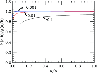
Figure 2: The ratio $h(a,b)/g(a/b)$ as function of $a/b$, for three values of $a$.

Finally, for the relation between the transverse to longitudinal growth rates according to modified Piwinski: note that for non-zero vertical dispersion the second term in the brackets of Eqs. 14 (but with $\eta^{2}_{x,y}/\beta_{x,y}$ replaced by ${\cal H}_{x,y}$), will tend to dominate over the first term, and the results become the same as for the B-M method.

In summary, we have shown that for high energy beams ($a$,$b\ll 1$), in rings with a standard type of storage ring lattice: if the parameter $d$ in P is chosen to give the same equivalent Coulomb log as in B-M, then the modified Piwinski solution agrees with the Bjorken-Mtingwa solution.

NUMERICAL COMPARISONBane et al.

We consider a numerical comparison between results of the general B-M method, the modified Piwinski method, and Eqs. 10,13. The example is the ATF ring with no coupling and vertical dispersion due to random orbit errors. For our example $\langle{\cal H}_{y}\rangle=17$ $\mu$m, yielding a zero-current emittance ratio of 0.7%; the beam current is 3.1 mA. The steady-state growth rates according to the 3 methods are given in Table I. We note that the Piwinski results are 4.5% low, and the results of Eqs. 10,13, agree very well with those of B-M. Finally note that, not only the growth rates, but even the differential growth rates—i.e. the growth rates as function of position along the ring—agree well for the three cases.

Table 1: Steady-state IBS growth rates for an ATF example including vertical dispersion due to random errors.

Method	$1/T_{p}$ [s-1]	$1/T_{x}$ [s-1]	$1/T_{y}$ [s-1]
Modified Piwinski	25.9	24.7	18.5
Bjorken-Mtingwa	27.0	26.0	19.4
Eqs. 10,13	27.4	26.0	19.4