Evolving Networks with Multi-species Nodes
and Spread in the Number of Initial Links

Abstract

We consider models for growing networks incorporating two effects not previously considered: (i) different species of nodes, with each species having different properties (such as different attachment probabilities to other node species); and (ii) when a new node is born, its number of links to old nodes is random with a given probability distribution. Our numerical simulations show good agreement with analytic solutions. As an application of our model, we investigate the movie-actor network with movies considered as nodes and actors as links.

I Introduction

It is known that many evolving network systems, including the world wide web, as well as social, biological, and communication systems, show power law distributions. In particular, the number of nodes with $k$ links is often observed to be $n_{k}\sim k^{-\nu}$, where $\nu$ typically varies from 2.0 to 3.1 Dorogovtsev1 . The mechanism for power-law network scaling was addressed in a seminal paper by Barabási and Albert (BA) who proposed Barabasi1 a simple growing network model in which the probability of a new node forming a link with an old node (the “attachment probability”) is proportional to the number of links of the old node. This model yields a power law distribution of links with exponent $\nu=3$. Many other works have been done extending this the model. For example Krapivsky and Redner Krapivsky1 provide a comprehensive description for a model with more general dependence of the attachment probability on the number $k$ of old node links. For attachment probability proportional to $A_{k}=ak+b$ they found that, depending on $b/a$, the exponent $\nu$ can vary from 2 to $\infty$. Furthermore, for $A_{k}\sim k^{\alpha}$, when $\alpha<1$, $n_{k}$ decays faster than a power law, while when $\alpha>1$, there emerges a single node which connects to nearly all other nodes. Other modifications of the model are the introduction of aging of nodes Dorogovtsev2 , initial attractiveness of nodes Dorogovtsev3 , the addition or re-wiring of links Albert1 , the assignment of weights to links Yook1 , etc.

We have attempted to construct more general growing network models featuring two effects which have not been considered previously: (i) multiple species of nodes [in real network systems, there may be different species of nodes with each species having different properties (e.g., each species may have different probabilities for adding new nodes and may also have different attachment probabilities to the same node species and to other node species, etc.)]. (ii) initial link distributions [i.e., when a new node is born, its number of links to old nodes is not necessarily a constant number, but, rather, is characterized by a given probability distribution $p_{k}$ of new links].

As an application of our model, we investigate the movie-actor network with movies considered as nodes and actors as links (i.e., if the same actor appears in two movies there is a link between the two movies movie ). Moreover, we consider theatrical movies and made-for-television movies to constitute two different species.

II Model

We construct a growing network model which incorporates multiple species and initial link probabilities. Given an initial network, we create new nodes at a constant rate. We let the new node belong to species $j$ with probability $Q^{(j)}$ ($\sum_{j}Q^{(j)}=1$). We decide how many links $l$ the new node establishes with already existing nodes by randomly choosing $l$ from a probability distribution $p^{(j)}_{l}$. Then, we randomly attach the new node to $l$ existing nodes with preferential attachment probability proportional to a factor $A^{(j,i)}_{k}$, where $k$ is the number of links of the target node of species $i$ to which the new node of species $j$ may connect. That is, the connection probability between an existing node and a new node is determined by the number of links of the existing node and the species of the new node and the target node.

As for the single species case Krapivsky1 , the evolution of this model can be described by rate equations. In our case the rate equations give the evolution of $N^{(i)}_{k}$, the number of species $i$ nodes that have $k$ links,

$$\frac{dN^{(i)}_{k}}{dt} = \sum^{S}_{j=1}Q^{(j)}\bar{k}^{(j)}\frac{\left[A^{(j,i)}_{k-1}N^{(i)}_{k-1}-A^{(j,i)}_{k}N^{(i)}_{k}\right]}{\sum_{m}\sum_{k}A^{(j,m)}_{k}N^{(m)}_{k}}$$ (1)

$$+Q^{(i)}p^{(i)}_{k},$$

where $S$ is the total number of species and $\bar{k}^{(j)}=\sum_{l}lp^{(j)}_{l}$ is the average number of new links to a new node of species $j$, and $t$ is normalized so that the rate of creation of new nodes is one per unit time. The term proportional to $A^{(j,i)}_{k-1}N^{(i)}_{k-1}$ accounts for the increase of $N^{(i)}_{k}$ due to the addition of a new node of species $j$ that links to a species $i$ node with $k-1$ connections. The term proportional to $A^{(j,i)}_{k}N^{(i)}_{k}$ accounts for the decrease of $N^{(i)}_{k}$ due to linking of a new species $j$ node with an existing species $i$ node with $k$ connections. The denominator, $\sum_{m}\sum_{k}A^{(j,m)}_{k}N^{(m)}_{k}$, is a normalization factor. If we add a new node with $l$ initial links, we have $l$ chances of increasing/decreasing $N^{(i)}_{k}$. This is accounted for by the factor $\bar{k}^{(j)}=\sum_{l}lp^{(j)}_{l}$ appearing in the summand of Eq. (1). The last term, $Q^{(i)}p^{(i)}_{k}$, accounts for the introduction of new nodes of species $i$. Since all nodes have at least one link, $N^{(i)}_{0}=0$.

III Analysis of the Model

Equation (1) implies that total number of nodes and total number of links increase at fixed rates. The total number of nodes of species $i$ increases at the rate $Q^{(i)}$. Thus

$$\sum_{k}N^{(i)}_{k}=Q^{(i)}t.$$ (2)

The link summation over all species $\sum_{i}\sum_{k}kN^{(i)}_{k}$ is twice the total number of links in the network. Thus

$$\sum^{S}_{i}\sum_{k}kN^{(i)}_{k}=2\left<\dot{k}\right>t,$$ (3)

where $\left<\dot{k}\right>=\sum_{i}\sum_{k}Q^{(i)}kp^{(i)}_{k}=\sum_{i}Q^{(i)}\bar{k}^{(i)}$. Solutions of (1) occur in the form(c.f., Krapivsky1 for the case of single species nodes),

$$N^{(i)}_{k}=n^{(i)}_{k}t,$$ (4)

where $n^{(i)}_{k}$ is independent of $t$. Eq. (1) yields

$$n^{(i)}_{k}=\frac{B^{(i)}_{k-1}n^{(i)}_{k-1}+Q^{(i)}p^{(i)}_{k}}{(B^{(i)}_{k}+1)},$$ (5)

where $B^{(i)}_{k}$ is

$$B^{(i)}_{k}=\sum^{S}_{j=1}Q^{(j)}\bar{k}^{(j)}\frac{A^{(j,i)}_{k}}{\sum_{m}\sum_{k}A^{(j,m)}_{k}n^{(m)}_{k}}.$$ (6)

To most simply illustrate the effect of spread in the initial number of links, we first consider the case of a network with a single species of node and with a simple form for the attachment $A_{k}=A^{(1,1)}_{k}$. In particular, we choose Krapivsky1 , $A_{k}=k+c$. (Note that by Eq. (1) this is equivalent to $A_{k}=ak+b$ with $c=b/a$.) Inserting this $A_{k}$ into Eq. (6), we obtain $\sum_{k}(k+c)n_{k}=2{\left<\dot{k}\right>}+cQ$ and $B_{k}=(k+c)/\eta$, where $\eta=(2{\left<\dot{k}\right>}+cQ)/{(Q\bar{k})}=2+c/{\bar{k}}\geq 2$. (Note that$\left<\dot{k}\right>=Q\bar{k}$ for the single species case.) Thus Eq. (5) yields

$$\left[(k+c)n_{k}-(k+c-1)n_{k-1}\right]+\eta n_{k}=\eta Qp_{k}.$$ (7)

Setting $p_{k}=p_{1}(k+c)^{-\beta}$, we can solve Eq. (7) for large $k$ by approximating the discrete variable $k$ as continuous, so that

$$(k+c)n_{k}-(k+c-1)n_{k-1}\cong\frac{d}{dk}[(k+c)n_{k}].$$ (8)

Solution of the resulting differential equation,

$$\frac{d}{dk}[(k+c)n_{k}]+\eta n_{k}=\eta Qp_{1}(k+c)^{-\beta},$$ (9)

for $n_{k}$ with $\beta\neq\eta+1$ consists of a homogeneous solution proportional to $(k+c)^{-(\eta+1)}$ plus the particular solution, $[\eta Qp_{1}/(\eta+1-\beta)](k+c)^{-\beta}$. For $\beta=\eta+1$ the solution is $n_{k}=\eta Qp_{1}(k+c)^{-(\eta+1)}\ln[d(k+c)]$, where $d$ is an arbitrary constant. Hence, for sufficiently large $k$ we have $n_{k}\sim k^{-(\eta+1)}$ if $\beta>\eta+1$, and $n_{k}\sim k^{-\beta}$ if $\beta<\eta+1$. Thus the result for $\beta>\eta+1$ is independent of $\beta$ and, for $c=0$, coincides with that give in Ref. Barabasi1 ($\eta+1=3$ when $c=0$). Solutions of Eq. (7) for $n_{k}$ versus $k$ in the range $1\leq k\leq 10^{4}$ are shown as open circles in Fig. 1(a) for initial link probabilities of the form

$$p_{k}=\left\{\begin{array}[]{ll}p_{1}k^{-1}&\text{ for $1\leq k\leq 10^{2}$}\\ p_{1}10^{2(\bar{\beta}-1)}k^{-\bar{\beta}}&\text{ for $k\geq 10^{2}$,}\end{array}\right.$$ (12)

which are plotted as solid lines in Fig. 1(a). The values of $\bar{\beta}$ used for the figure are $\bar{\beta}=0.5,1,2,3,4$, and $\infty$ ($\bar{\beta}=\infty$ corresponds to $p_{k}\equiv 0$ for $k>10^{2}$). For clarity $n_{k}$ has been shifted by a constant factor so that $n_{1}$ coincides with the corresponding value of $p_{1}$. Also, to separate the graphs for easier visual inspection, the value of $p_{1}$ for successive $\bar{\beta}$ values is changed by a constant factor [since (7) is linear, the form of the solution is not effected]. We note from Fig. 1(a) that $n_{k}$ follows $p_{k}$ for $k<10^{2}$ in all cases. This is as expected, since $p_{k}$ decreases slower than $k^{-3}$ in this range. Furthermore, $n_{k}$ very closely follows $p_{k}$ for $k>10^{2}$ for $\bar{\beta}=0.5,1.0,2.0$. As $\bar{\beta}$ increases deviations of $n_{k}$ from $p_{k}$ in $k>10^{2}$ become more evident, and the large $k$ asymptotic $k^{-3}$ dependence is observed. Thus, if $p_{k}$ decreases sufficiently rapidly, then the behavior of $n_{k}$ is determined by the growing network dynamics, while, if $p_{k}$ decreases slowly, then the behavior of $n_{k}$ is determined by $p_{k}$.

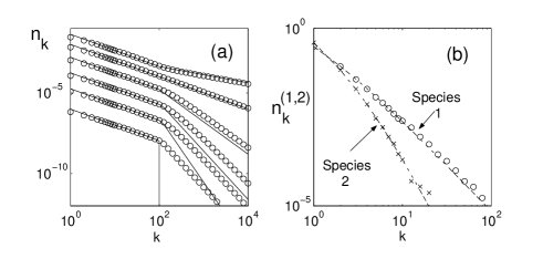
Figure 1: (a) $n_{k}$ and $p_{k}$ versus $k$ for the single species network model. Solid lines are the initial link probability $p_{k}$ and circles are the $n_{k}$ obtained from Eq. (7). (b) $n^{(1)}_{k}$ and $n^{(2)}_{k}$ versus $k$ for the two species network model. Circles (species $1$) and crosses (species $2$) are log-binned data from our numerical simulation. The total number of nodes in our numerical network system is $10^{6}$. The dashed lines are solutions obtained from (5) and (15).

To simply illustrate the effect of multiple species we now consider a growing two species network with $p_{k}=\delta_{1,k}$ (i.e., $p_{k}=0$ for $k\geq 2$). Then, Eq. (6) becomes

$$B^{(1)}_{k} = \frac{Q^{(1)}A^{(1,1)}_{k}}{\sum_{m}\sum_{k}A^{(1,m)}_{k}n^{(m)}_{k}}+\frac{Q^{(2)}A^{(2,1)}_{k}}{\sum_{m}\sum_{k}A^{(2,m)}_{k}n^{(m)}_{k}},$$ (13a)

$$B^{(2)}_{k} = \frac{Q^{(1)}A^{(1,2)}_{k}}{\sum_{m}\sum_{k}A^{(1,m)}_{k}n^{(m)}_{k}}+\frac{Q^{(2)}A^{(2,2)}_{k}}{\sum_{m}\sum_{k}A^{(2,m)}_{k}n^{(m)}_{k}},$$ (13b)

where $\sum_{m}$ represents summation of species $1$ and $2$ nodes.

In order to illustrate the model with our numerical simulations, we specialize to a specific case. We choose attachment coefficients $A^{(1,1)}_{k}=ak$, $A^{(1,2)}_{k}=ak$, $A^{(2,1)}_{k}=bk$, and $A^{(2,2)}=0$. Thus a new species $1$ node connects to either existing species $1$ nodes and species $2$ nodes with equal probability, while a new species $2$ node can connect to existing species $1$ nodes only. Therefore, the first summation term in Eq. (13), ${\sum_{m}\sum_{k}A^{(1,m)}_{k}n^{(m)}_{k}}$, becomes $a\sum_{k}(kn^{(1)}_{k}+kn^{(2)}_{k})$, which is $a$ times the total increase of links at each time $a\times 2(Q^{(1)}+Q^{(2)})$. Recall that $Q^{(1)}+Q^{(2)}=1$. In order to calculate the second summation term in Eq. (13), ${\sum_{m}\sum_{k}A^{(2,m)}_{k}n^{(m)}_{k}}=b\sum_{k}kn^{(1)}_{k}$, we define a parameter $\gamma$ that is the ratio of the total number of links of species $1$ to the total number of links in the network. Since the probability of linking a new species $1$ node to existing species $1$ nodes is determined by the total number of links of species $1$, this probability is exactly same as $\gamma$. Thus, if we add a new species $1$ node, the number of links of species $1$ increases by $Q^{(1)}$ due to the new node and by $\gamma Q^{(1)}$ due to the existing species $1$ nodes that become connected with the new node, while the number of links of species $2$ increases by $(1-\gamma)Q^{(1)}$. But, if we add a new species $2$ node, the numbers of links increases by $Q^{(2)}$ for both species because a new species $2$ node can link to species $1$ nodes only. Thus, the increase of species $1$ links is $(1+\gamma)Q^{(1)}+Q^{(2)}$ and that of species $2$ links is $(1-\gamma)Q^{(1)}+Q^{(2)}$. Since $\gamma$ is the ratio of the number of species $1$ links to the total number of links, $\gamma=[(1+\gamma)Q^{(1)}+Q^{(2)}]/2$ or

$$\gamma=\frac{1}{2-Q^{(1)}}.$$ (14)

With this $\gamma$, Eq. (13) becomes

$$B^{(1)}_{k} = \frac{Q^{(1)}}{2}k+\frac{Q^{(2)}(2-Q^{(1)})}{2}k=\frac{k}{\eta^{(1)}},$$ (15a)

$$B^{(2)}_{k} = \frac{Q^{(1)}}{2}k=\frac{k}{\eta^{(2)}}.$$ (15b)

where obtain $\eta^{(1)}=2/[Q^{(1)}+Q^{(2)}(2-Q^{(1)})]$ and $\eta^{(2)}=2/Q^{(1)}$.

Proceeding as for the single species case, we approximate (5) by an ordinary differential equation (c.f., Eq. (9)) to obtain $n^{(i)}_{k}\sim k^{-(1+\eta^{(i)})}$. As an example, we set $Q^{(1)}=Q^{(2)}=0.5$, in which case Eqs. (15) give exponents $1+\eta^{(1)}=2.6$ and $1+\eta^{(2)}=5$. In Fig. 1(b) we plot, for this case, the analytic solution obtained from (5) and (15) as dashed lines, and the results of numerical simulations as open circles and pluses. The simulation results, obtained by histogram binning with uniform bin size in $\log k$, agree with the analytic solutions, and both show the expected large $k$ power law behaviors, $n^{(1)}_{k}\sim k^{-2.6}$ and $n^{(2)}_{k}\sim k^{-5}$.

IV The Movie-Actor Network

We now investigate the movie-actor network. We collected data from the Internet Movie Data Base (IMDB) web site Imdb . The total number of movies is 285,297 and the total number of actors/actresses is 555,907. Within this database are 226,325 theatrical movies and 24,865 made for television movies. The other movies in the database are made for television series, video, mini series, and video games. In order to get good statistics, we choose only theatrical and television movies made between 1950 to 2000. Thus we have two species of movies. We also consider only actors/actresses from these movies. We consider two movies to be linked if they have an actor/actress in common. We label the theatrical movies species $1$, and the made for television movies species $2$.

In order to apply our model, Eq. (1), we require as input $Q^{(j)},p^{(j)}_{k}$ and $A^{(j,i)}_{k}$ which we obtain from the movie-actor network data. We take $Q^{(1)}$ and $Q^{(2)}$ to be, respectively, the fractions of theatrical and made for television movies in our data base. We obtain $Q^{(1)}=0.83$ and $Q^{(2)}=0.17$. We now consider $p^{(j)}_{k}$. Suppose a new movie is produced casting $r$ actors. For each actor $s$ $(s=1,2,...,r)$ let $l_{s}$ denote the number of previous movies in which that actor appeared. Then the total number of the initial links of the new movie is $\sum_{s}l_{s}$. From histograms of this number, we obtain (Figs. 2) the initial link probability distributions $p^{(j)}_{k}$.

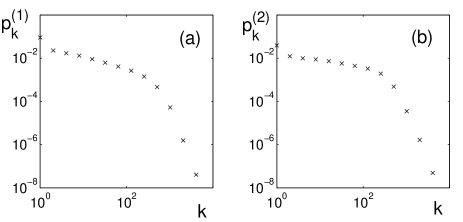
Figure 2: The initial link probability distributions $p_{k}$ of (a) theatrical movies and (b) television movies. These plots are obtained using bins of equal width in $\log k$ and dividing the number of nodes in each bin by the product of the bin width in $k$ (which varies from bin to bin) and the total number of nodes.

The attachment $A^{(j,i)}_{k}$ can be numerically obtained from data via,

$$A^{(j,i)}_{k}\sim\frac{\left<\Delta(j;i,k)\right>}{\delta t},$$ (16)

where $\Delta(j;i,k)$ is the increase during a time interval $\delta t$ in the number of links between old species $i$ nodes that had $k$ links and new species $j$ nodes, and $<...>$ is an average over all such species $i$ nodes Jeong1 . In the movie network, we count all movies and links from 1950 to 1999, and measure the increments in the number of links for a $\delta t$ of one year. We obtain attachment coefficient $A^{(1,1)}_{k}\sim 0.10k^{0.59}$ and $A^{(1,2)}_{k}\sim 0.04k^{0.85}$ for theatrical movies, and $A^{(2,1)}_{k}0\sim 0.02k^{0.71}$ and $A^{(2,2)}_{k}\sim 0.04k^{0.77}$ for television movies. See Fig. 3.

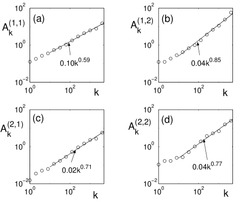
Figure 3: Attachment coefficients for theatrical movies (a) $A^{(1,1)}_{k}$ and (b) $A^{(1,2)}_{k}$, and for television movies (c) $A^{(2,1)}_{k}$ and (d) $A^{(2,2)}_{k}$. All data are obtained using log-binning without normalization (see caption to Fig. 2).

Incorporating these results for $Q^{(i)}$, $p^{(i)}_{k}$ and $A^{(j,i)}_{k}$ in our multi-species model, Eq. (1), we carry out numerical simulations as follows: (i) We add a new movie at each time step. We randomly designate each new movie as a theatrical movie with probability $Q^{(1)}=0.83$ or a television movie with probability $Q^{(2)}=0.17$. (ii) With initial link probability $p^{(j)}_{k}$, we randomly choose the number of connections to make to old movies. (iii) We then use the attachment $A^{(j,i)}_{k}$ to randomly choose connections of new species $j$ movie to old species $i$ movies. (iv) We repeat (i)-(iii) adding 100,000 new movies, and finally calculate the probability distributions of movies with $k$ links.

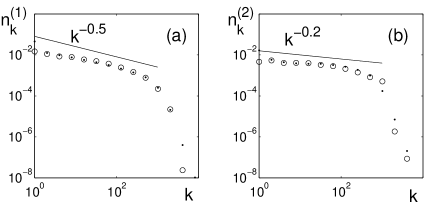
Figure 4: The probability distributions $n^{(i)}_{k}$ of movies that have $k$ links; (a) theatrical movies $n^{(1)}_{k}$ and (b) television movies $n^{(2)}_{k}$. Dots are $n^{(i)}_{k}$ obtained from the movie network while circles are from numerical simulation using $Q^{(j)}$ obtained from our data base, $p^{(j)}_{k}$ in Fig. 2 and $A^{(j,i)}_{k}$ in Fig. 3. All data are obtained using log-binning (see caption to Fig. 2).

Figure 4 shows $n^{(i)}_{k}$ versus $k$ obtained from our movie-actor network data base (dots) and from numerical simulations using Eq.(1) (open circles) with our empirically obtained results for $Q^{(j)}$, $p^{(j)}_{k}$, and $A^{(j,i)}_{k}$. The results are are roughly consistent with the existence of two scaling regions twoscale1 . For small $k$ $(k\lesssim 10^{2}$) the two species exhibit slow power law decay with different exponents, $n^{(1)}_{k}\sim k^{-0.5}$, $n^{(2)}_{k}\sim k^{-0.2}$, while for large $k$ the probabilities decay much more rapidly. Indeed, the results of Krapivsky1 suggest that the decay should be exponential for large $k$ since the attachment $A^{(j,i)}_{k}$ grow sub-linearly with $k$. We showed in Sec. III for the single species model with a linear attachment $A_{k}\sim k$ that $n_{k}$ follows $p_{k}$ when $p_{k}$ decays slowly, while $n_{k}$ is independent of $p_{k}$ when $p_{k}$ decays sufficiently quickly. As we will later show, this feature is also applicable to multi-species networks with nonlinear attachments. As seen in Figs. 5(a) and 5(b), $n^{(i)}_{k}$ follows $p^{(i)}_{k}$ in the small $k$ region. However, it is not clear whether $n^{(i)}_{k}$ follows $p^{(i)}_{k}$ in the large $k$ region. In order to check the behavior of $n^{(i)}_{k}$ in this region, we carried out another numerical simulation using an initial link probability $\bar{p}^{(i)}_{k}$ which is cut off at $k=50$. That is, $\bar{p}^{(i)}_{k}=p^{(i)}_{k}/\sum\bar{p}^{(i)}_{k}$ when $k\leq 50$ and $\bar{p}^{(i)}_{k}=0$ when $k>50$. Using $\bar{p}^{(i)}_{k}$ in place of $p^{(i)}_{k}$, we obtain from our simulation corresponding data, $\bar{n}^{(i)}_{k}$ versus $k$, which are shown in Figs. 5(c) and 5(d) as filled in circles. For comparison the data for $n^{(i)}_{k}$ from Figs. 5(a) and 5(b) are plotted in Figs. 5(c) and 5(d) as open circles. It is seen that the cutoff at $k=50$ induces a substantial change in the distribution of the number of links for $k>50$. Thus it appears that, in the range tested, the large $k$ behavior of the movie-actor network is determined by the initial link probability $p^{(i)}_{k}$ rather than by the dynamics of the growing network.

In conclusion, in this paper we propose a model for a multi-species network with variable initial link probabilities. We have investigated the movie-actor network as an example. We believe that the effect of multiple species nodes may be important for modeling other complicated networks (e.g., the world wide web can be divided into commercial sites and educational or personal sites). We also conjecture that the initial link probability is a key feature of many growing networks.

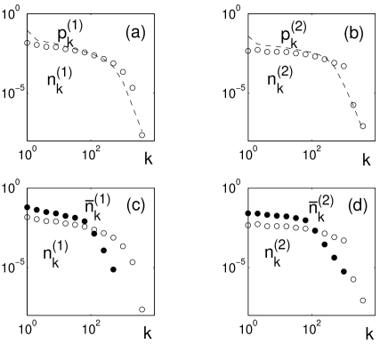
Figure 5: (a) and (b) are $n^{(i)}_{k}$ (circles) obtained from numerical simulations using $p^{(i)}_{k}$ (dashed lines), while (c) and (d) show $n^{(i)}_{k}$ from (a) and (b) (open circles) plotted with results denoted $\bar{n}^{(i)}_{k}$ (filled circles) from simulation using a cutoff initial link probability $\bar{p}^{(i)}_{k}$ (where $\bar{p}^{(i)}_{k}=p^{(i)}_{k}/\sum\bar{p}^{(i)}_{k}$ when $k\leq 50$ and $\bar{p}^{(i)}_{k}=0$ when $k>50$). All data are obtained using log-binning (see caption to Fig. 2).

References

- (1) S.N. Dorogovtsev and J.F.F. Mendes, ArXiv:cond-mat/0106144 v1 7 Jun 2001. They summarize values of for several network systems in Table I.
- (2) A.-L. Barabási and R. Albert, Science 286, 509(1999).
- (3) P.L. Krapivsky and S. Redner, Phys. Rev. E 6306(6):6123 (2001); See also P.L. Krapivsky, S. Render, and F. Leyvraz, Phys. Rev. Lett. 85, 4629(2000).
- (4) S.N. Dorogovtsev, J.F.F. Mendes, and A.N. Samukhin Phys. Rev. Lett. 85, 4633(2000).
- (5) S.N. Dorogovtsev and J.F.F. Mendes, Phys. Rev. E 62, 1842(2000).
- (6) R. Albert and A.-L. Barabási, Phys. Rev. Lett. 85, 5234(2000).
- (7) S.H. Yook, H. Jeong, and A.-L. Barabási, Phys. Rev. Lett. 86, 5835(2001).
- (8) Barabási and Albert also investigated the movie-actor network. However, they consider actors as nodes that are linked if they are cast in the same movie. See Ref. Barabasi1 and Ref. Albert1 .
- (9) The Internet Movie Database, http://www.imbd.com
- (10) The technique we use for obtaining is similar to that used by H. Jeong et al. who presume single species situations (in which case the superscripts , do not apply). [H. Jeong, Z. Néda, and A.-L. Barabási, ArXiv:cond-mat/0104131 v1 7 Apr 2001.]
- (11) Similar observations suggesting two scaling regions have also been recently observed in other cases of growing networks. Barabási et al. investigated the scientific collaboration network [A.-L. Barabási, et al., ArXiv:cond-mat/0104162 v1 10 Apr 2001]. They argue that a model in which links are continuously created between existing nodes explains the existence of two scaling regions in their data. Vazquez investigated the citation network of papers (nodes) and authors (links) for Phys. Rev. D and found two scalings in its in-degree distribution. See A. Vazquez, ArXiv:cond-mat/0105031 v1 2 May 2001.