Transverse self-fields within an electron bunch moving in an arc of a circle

Abstract

As a consequence of motions driven by external forces, self-fields (which are different from the static case) originate within an electron bunch. In the case of magnetic external forces acting on an ultrarelativistic beam, the longitudinal self-interactions are responsible for CSR (Coherent Synchrotron Radiation)-related phenomena, which have been studied extensively. On the other hand, transverse self-interactions are present too. At the time being, existing theoretical analysis of transverse self-forces deal with the case of a bunch moving along a circular orbit only, without considering the situation of a bending magnet with a finite length. In this paper we propose an electrodynamical analysis of transverse self-fields which originate, at the position of a test particle, from an ultrarelativistic electron bunch moving in an arc of a circle. The problem will be first addressed within a two-particle system. We then extend our consideration to a line bunch with a stepped density distribution, a situation which can be easily generalized to the case of an arbitrary density distribution. Our approach turns out to be also useful in order to get a better insight in the physics involved in the case of simple circular motion and in order to address the well known issue of the partial compensation of transverse self-force.

DEUTSCHES ELEKTRONEN-SYNCHROTRON

DESY 02-048

May 2002

I INTRODUCTION

When an electron bunch undergoes a motion under the influence of external forces, the particles within the bunch become sources of self-fields which are different from the static case and which obey the usual Lienard-Wiechert expressions.

These self-fields feed back on the particle dynamics, which often makes the description of the evolution of the system a problem without easy solution.

Many electrodynamical systems fit in the latter description. In all these systems one can recognize two separate aspects in the evolution issue: a dynamical one, which is governed by the equation of motion, and an electrodynamical one, which is taken care of by Maxwell equations. The solution to the evolution problem is obtained when one is able to solve simultaneously both equations: this is, for example, what self-consistent computer codes strive for. An example of such self-consistent, numerical solutions is given (see ROTH ) by the program TRAFIC⁴ (which will be employed in this paper to provide cross-checks with analytical results). Although TRAFIC⁴ and other codes are able to provide quite reliable results for a number of evolution problems, a separate study of their dynamical and electrodynamical aspects, which can be achieved by means of theoretical analysis, is necessary in order to get a good understanding of the physics involved, and to provide benchmark and cross-checks for simulations (and, at an earlier stage, to build correct simulations too).

Moreover, it often happens that this kind of theoretical analysis can be directly applied in order to get good practical solutions for the problem at least in a narrow region of the parameters which specify the system setup. The results can, then, be used for quick estimations of the magnitude of the effects under investigation.

Let us restrict our attention to the case of self-fields within an ultrarelativistic electron bunch driven by external forces of magnetic nature.

The self-interaction in the longitudinal direction (parallel, at any time, to the velocity vector by definition) is responsible for the energy exchange between the system and the acceleration field and for all CSR (Coherent Synchrotron Radiation)-related phenomena, which have been studied extensively elsewhere (see, among the others, ROTH … BORL ).

These investigations are important in view of the need for very high-peak current, low emittance beams for self-amplified spontaneous emission (SASE)-free-electron-lasers operating in the x-ray region (see, among the others, XRAY ). Similar beams are also being considered for production of femtosecond radiation pulses by simpler schemes based on Cherenkov and Transition Radiation WALTER : production and utilization of such kind of beams may prove difficult due to self-field collective effects. Indeed, these effects may spoil the required high brightness of the electron beam, which is a matter of major concern among people involved this kind of physics research.

The study of self-forces in the transverse direction is important for the same reasons. They were first addressed, in the case of a circular motion, and from an electrodynamical viewpoint, in TALM . Further analysis (RUI2 , LEE … STUP ) consider, again, the case of circular motion both from an electrodynamical and a dynamical viewpoint and in the approximation of a rigid bunch: at the time being, existing theoretical analysis of transverse self-forces deal with the case of circular orbit only, without considering transient collective phenomena.

In this paper we propose a fully electrodynamical analysis of transverse self-fields originating, at the position of a test particle, from an ultrarelativistic electron bunch moving in an arc of a circle, thus treating for the first time, besides the basic situation of circular motion, also the case of transient between a straight line and a hard-edge magnet (and, vice versa, from a bend to a straight line).

Consistently with the choice to analyze the electrodynamical aspect of the problem only, a zero energy-spread will be understood when considering the evolution of an electron bunch. As underlined before, although the results obtained can be directly applied, from a practical viewpoint, only in the case in which the zero energy-spread hypothesis is verified a posteriori, the outcomes of this paper are important to get a good insight if the physics of the problem, and to provide benchmark and cross-checks for simulations.

Firstly, a two-particle model is adopted in order to study the transverse force produced by a single particle, and then, by summing up all the contributions from different electrons, the case of a line-bunch model characterized by a rectangular density distribution is analyzed: this can, in fact, be easily generalized to the case of an arbitrary density distribution.

Besides providing results in the case of a finite hard-edge bending magnet, our approach turns also useful in order to get a better insight of the physics involved in the case of simple circular motion.

Moreover, our results give us a better understanding (although one has to take into account, here, dynamical aspects as well as electrodynamical ones) of the partial compensation between transverse self-force and gradient of the potential energy deviation from the nominal value.

We will discuss the limits of applicability of our model, with respect to the transverse beam size, $h$, in Section III). Within such applicability limits, we find results which are independent of the bunch transverse dimension.

The paper is organized as follows. The transverse interaction between two electrons moving on a circle, together with a simple dynamical interpretation is treated in Section II. In Section III, we deal with a stepped-profile electron bunch interacting with a test particle again on a circle, and discuss also the applicability region of the line model. Transient behavior (from straight to circular path and vice versa) for the transverse self-forces between two particles are then studied in Section IV. Results for the transient of a stepped-profile bunch are given in Section V, where a treatment for the case of a more generic bunch density is also proposed. A regularization technique for cancelling the singularity in the expression for the transverse force (which always arises in the limit of a near-zero distance between test particle and sources) is then applied. In Section VI we will deal with the well-known issue of the partial compensation of transverse self-force. Finally, in Section VII, we come to a summary of the obtained results and to conclusions.

II TRANSVERSE INTERACTION BETWEEN TWO ELECTRONS MOVING IN A CIRCLE

Let us begin our study considering the steady case of two electrons moving on a circle of radius $R$. The electro-magnetic force which one of the two particles (designated with ”T”, i.e. the test particle) feels, due to the interaction with the other one (designated with ”S”, i.e. the source particle), is given by

$${\bm{F}}({\bm{r_{\mathrm{T}}}},t)=e{\bm{E}}({\bm{r_{\mathrm{T}}}},t)+ec{\bm{\beta_{\mathrm{T}}}}\times{\bm{B}}({\bm{r_{\mathrm{T}}}},t),$$ (3)

where ${\bm{r_{\mathrm{T}}}}$ is the position of the test particle, $e$ is the electron charge with its own (negative) sign, $\bm{\beta_{\mathrm{T}}}$ is the velocity of the test particle normalized to the speed of light, $c$, while $\bm{E}({\bm{r_{\mathrm{T}}}},t)$ and $\bm{B}({\bm{r_{\mathrm{T}}}},t)$ are, respectively, the electric and the magnetic field generated at a given time $t$ by the source particle S, at the position of the test particle T, namely

$${\bm{E}}({\bm{r_{\mathrm{T}}}},t)={e\over{4\pi\varepsilon_{\mathrm{0}}}}\Biggl{\{}{1\over\gamma_{\mathrm{S}}^{2}}{{\bf{\hat{n}}}-{\bm{\beta_{\mathrm{S}}}}\over{R_{\mathrm{ST}}^{2}\left({1-{\bf{\hat{n}}}\cdot{\bm{\beta_{\mathrm{S}}}}}\right)^{3}}}$$

(4)

$$+{1\over c}{{\bf{\hat{n}}}\times\left[{\left({{\bf{\hat{n}}}-{\bm{\beta_{\mathrm{S}}}}}\right)\times{\dot{\bm{\beta}}_{\bm{\mathrm{S}}}}}\right]\over{R_{\mathrm{ST}}\left({1-{\bf{\hat{n}}}\cdot{\bm{\beta_{\mathrm{S}}}}}\right)^{3}}}\Biggr{\}}~{}$$ (5)

and

$${\bm{B}}({\bm{r_{\mathrm{T}}}},t)={1\over c}{\bf{\hat{n}}}\times{\bm{E}}({\bm{r_{\mathrm{T}}}},t)~{}.$$ (6)

Here ${\bm{\beta_{\mathrm{S}}}}$ and ${\dot{\bm{\beta}}_{\bm{\mathrm{S}}}}$ are, respectively, the dimensionless velocity and its time derivative at the retarded time $t^{\prime}$, $R_{\mathrm{ST}}$ is the distance between the retarded position of the source particle and the present position of the test electron, $\bf{\hat{n}}$ is a unit vector along the line connecting those two points and $\gamma_{\mathrm{S}}$ is the usual Lorentz factor referred to the source particle at the retarded time $t^{\prime}$.

The transverse direction (on the orbital plane) is, by definition, orthogonal to $\bm{\beta_{\mathrm{T}}}$. The transverse component of Eq. (3) can be written as the sum of contributions from the velocity (”C”, Coulomb) and the acceleration (”R”, Radiation) fields, namely

$${\bm{F_{\bot}}}({\bm{{r_{\mathrm{T}}}}},t)={\bm{F_{\mathrm{\bot C}}}}({\bm{r_{\mathrm{T}}}},t)+{\bm{F_{\mathrm{\bot R}}}}({\bm{r_{\mathrm{T}}}},t),$$ (7)

where

$${\bm{F}_{\bm{\mathrm{\bot C}}}}({\bm{r_{\mathrm{T}}}},t)={e^{2}\over{4\pi\varepsilon_{\mathrm{0}}}}{{\bf{n_{\bot}}}\left(1-{\bm{\beta_{\mathrm{S}}}}\cdot{\bm{\beta_{\mathrm{T}}}}\right)-{\bm{\beta_{\mathrm{\bot S}}}}\left(1-{\bf{\hat{n}}}\cdot{\bm{\beta_{\mathrm{T}}}}\right)\over{\gamma_{\mathrm{S}}^{2}R_{\mathrm{ST}}^{2}\left(1-{\bf{\hat{n}}}\cdot{\bm{\beta_{\mathrm{S}}}}\right)^{3}}}$$ (8)

and

$${\bm{F}_{\bm{\mathrm{\bot R}}}}({\bm{r_{\mathrm{T}}}},t)={e^{2}\over{4\pi\varepsilon_{\mathrm{0}}}}\Bigg{[}{{\bf{n_{\bot}}}\left({\bf{\hat{n}}}\cdot{{\dot{\bm{\beta}}_{\bm{\mathrm{S}}}}}\right)\left(1-{\bm{\beta_{\mathrm{S}}}}\cdot{\bm{\beta_{\mathrm{T}}}}\right)-{\bm{\beta_{\mathrm{\perp S}}}}\left({\bf{\hat{n}}}\cdot{{\dot{\bm{\beta}}_{\bm{\mathrm{S}}}}}\right)\left(1-{\bf{\hat{n}}}\cdot{\bm{\beta_{\mathrm{T}}}}\right)\over{R_{\mathrm{ST}}\left(1-{\bf{\hat{n}}}\cdot{\bm{\beta_{\mathrm{S}}}}\right)^{3}}}-{\dot{\bm{\beta}}_{\bm{\mathrm{\perp T}}}\left(1-{\bf{\hat{n}}}\cdot{\bm{\beta_{\mathrm{T}}}}\right)+{\bf{\hat{n}_{\perp}}}\left({\bm{\beta_{\mathrm{T}}}}\cdot{{\dot{\bm{\beta}}_{\bm{\mathrm{S}}}}}\right)\over{R_{\mathrm{ST}}\left(1-{\bf{\hat{n}}}\cdot{\bm{\beta_{\mathrm{S}}}}\right)^{2}}}\Bigg{]}\;.$$ (9)

Let us first consider the case in which the test particle is in front of the source. In this case, referring to Fig. 1, we can define with $\Delta s$ the curvilinear distance between the present position of the test and of the source particle; $\phi$ will indicate, instead, the angular distance between the retarded position of the source and the present position of the test electron, and it will be designated as the retarded angle.

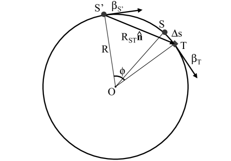
Figure 1: Geometry for the two-particle system in the steady state situation, with the test particle ahead of the source. Here T is the present position of the test particle, S is the present position of the source, while S’ indicates the retarded position of the source.

In the following we will assume $\beta_{\mathrm{S}}=\beta_{\mathrm{T}}=\beta$. This hypothesis will naturally lead, further on, to the assumption of a zero energy-spread when one considers the evolution of an electron bunch, and, as already discussed in Sec. I, it is consistent with our choice to analyze only the electrodynamical aspect of the problem. Upon this we can write Eq. (8) and Eq. (9) in the following way:

$${F_{\mathrm{\bot C}}}={e^{2}\over{4\pi\varepsilon_{\mathrm{0}}}}{1+\beta^{2}-2\beta\cos(\phi/2)\over{4R^{2}\gamma^{2}\sin(\phi/2)(1-\beta\cos(\phi/2))^{3}}}~{},$$ (10)

$${F_{\mathrm{\bot R}}}={e^{2}\over{4\pi\varepsilon_{\mathrm{0}}}}{\beta^{2}\over{2R^{2}}}\Bigg{[}{1\over{\sin(\phi/2)\left(1-\beta\cos(\phi/2)\right)}}$$

(11)

$$-{(1-\beta^{2})\sin{\phi/2}\over{\left(1-\beta\cos(\phi/2)\right)^{3}}}\Bigg{]}~{}.$$ (12)

If we now assume a small retarded angle ($\phi\ll 1$), which is justified in the ultrarelativistic case, we can expand Eq. (10) and Eq. (12) to the second non-vanishing order in $\phi$ thus obtaining

$${F_{\mathrm{\bot C}}}\simeq{e^{2}\gamma^{3}\over{4\pi\varepsilon_{\mathrm{0}}R^{2}}}\Phi_{\mathrm{C}}(\hat{\phi})$$ (13)

and

$${F_{\mathrm{\bot R}}}\simeq{e^{2}\gamma^{3}\over{4\pi\varepsilon_{\mathrm{0}}R^{2}}}\Phi_{\mathrm{R}}(\hat{\phi})~{},$$ (14)

where we define $\Phi_{\mathrm{C}}$ and $\Phi_{\mathrm{R}}$ as

$$\Phi_{\mathrm{C}}(\hat{\phi})={\hat{\phi}^{2}\over{\hat{\phi}(1+\hat{\phi}^{2}/4)^{3}}}$$ (15)

and

$$\Phi_{\mathrm{R}}(\hat{\phi})={2-\hat{\phi}^{2}+\hat{\phi}^{4}/8\over{\hat{\phi}(1+\hat{\phi}^{2}/4)^{3}}}~{}.$$ (16)

Here and above $\hat{\phi}=\gamma\phi$. This normalization choice, already treated in SALLONG , is quite natural, $1/\gamma$ being the synchrotron radiation formation-angle at the critical wavelength. In the derivation of Eq. (13) and Eq. (14) (and in the following, too) we understood $\hat{\phi}\gg 1/\gamma$, which is again justified by the ultrarelativistic approximation. Moreover, it is important to realize that the assumption $\phi\ll 1$ is by no means a restrictive one, since it keeps open the possibility of comparing $\phi$ with the formation angle $1/\gamma$ (note that a deflection angle smaller or bigger than $1/\gamma$ is characteristic of the cases, respectively, of undulator or synchrotron radiation).

The following expression can be then trivially derived, which is valid for the total transverse force felt by the test particle

$${F_{\mathrm{\bot}}}\simeq{e^{2}\gamma^{3}\over{4\pi\varepsilon_{\mathrm{0}}R^{2}}}\Phi(\hat{\phi})~{},$$ (17)

where $\Phi$ is defined by

$$\Phi(\hat{\phi})={2+\hat{\phi}^{4}/8\over{\hat{\phi}(1+\hat{\phi}^{2}/4)^{3}}}~{},$$ (18)

Note that Eq. (18) is completely independent of the parameters of the system: it is then straightforward to study the asymptotic behaviors of $\Phi$. In order to do so, just remember that the retardation condition linking $\Delta s$ and $\phi$ is given by (see SALLONG )

$$\Delta s=R\phi-2\beta R\sin{\phi\over{2}}~{},$$ (19)

or its approximated form

$$\Delta s=(1-\beta)R\phi+{R\phi^{3}\over{24}}~{}.$$ (20)

It is now evident that $\Phi(\Delta\hat{s})\rightarrow 1/(3\Delta\hat{s})$ when $\hat{\phi}\gg 1$ and $\Phi(\Delta\hat{s})\rightarrow 1/(\Delta\hat{s})$ when $\hat{\phi}\ll 1$, having introduced the normalized quantity $\Delta\hat{s}=(\gamma^{3}/R)\Delta s$. This normalization choice is linked to the fact that the critical synchrotron radiation wavelength, $R/\gamma^{3}$, is also the minimal characteristic distance of our system: two particles nearer than such a distance can be considered as a single one radiating, up to the critical frequency, with charge $2e$ (see SALLONG ).

The asymptotic behavior above suggests to study the function $\Phi(\Delta\hat{s})\Delta\hat{s}$. We plotted such a function in Fig. 2 (together with the radiative contribution alone) for values of $\Delta\hat{s}$ running from 0 to 5.

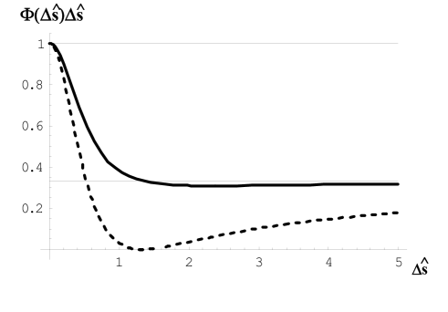
Figure 2: Plot of $\Phi(\Delta\hat{s})\Delta\hat{s}$ (solid line) and comparison with the asymptotic values, $1$ and $1/3$. The dashed line shows the radiative contribution $\Phi_{\mathrm{R}}(\Delta\hat{s})\Delta\hat{s}$ alone.

It is interesting to underline the fact that, as one can see from Fig. 2, the transverse force is always centrifugal, for any distance between the two particles. This fact can be explained by means of a simple relativistic argument which holds, qualitatively, for all particle distances: in order to build the two-particle system, i.e. to bring them together, one needs to work against the electromagnetic field. Then, the total mass of the system accounts for this interaction energy too, and is therefore bigger than the simple sum of the particles masses. Hence, also the equilibrium orbit radius must be bigger than $R$, and a centrifugal self-force is to be expected.

It is also worthwhile to note that $\Phi_{\mathrm{R}}$ has the same asymptotic behavior as $\Phi$, and that $\Phi_{\mathrm{C}}$ gives important contributions to $\Phi$ only for values between the two asymptotes (see Fig. 2). This may find intuitive explanation in the following reasoning. As is well known (see, for example, JACK ), the velocity field of an ultrarelativistic electron is radial, with respect to the ”virtual” position which the particle would assume if it moved with constant velocity starting from the retarded point, but the line forces are not isotropically distributed, and resemble more and more the plane wave configuration as $\beta\rightarrow c$. Therefore, the test particle is influenced by the velocity field of the source particle only when such a field ”shines right on the test electron” (quoted from RUI1 ), which does not happen for asymptotic values of $\hat{\phi}$.

Let us now analyze, in the framework of our line model, the case in which the source particle is in front of the test particle. The geometry is qualitatively sketched in Fig. 3.

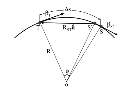
Figure 3: Geometry for the two-particle system in the steady state situation, with the source particle ahead of the test one. Here T is the present position of the test particle, S is the present position of the source, while S’ indicates the retarded position of the source.

The difference with respect to the situation in which the test electron is in front of the source is that the test electron ”runs against” the electromagnetic signal emitted by the source, while in the other case it just ”runs away” from it. Therefore the relative velocity between the signal and the test electron is equal to $(1+\beta)c$, instead of $(1-\beta)c$ in the other situation. Hence the retardation condition reads

$$\Delta s=R\phi+2\beta R\sin{\phi\over{2}}$$ (21)

or, solved for $\phi$ in its approximated form,

$$\phi\simeq{\Delta s\over{R(1+\beta)}}~{}.$$ (22)

In this situation, $\bm{\beta_{\mathrm{S}}}$ is almost parallel to (and equal to) $\bm{\beta_{\mathrm{T}}}$ and antiparallel to $\hat{n}$: it turns out that the only important contribution to the transverse force is given by the second term on the right side of Eq. (9), and it is easy to check that

$${F_{\mathrm{\bot}}}\simeq{e^{2}\over{4\pi\varepsilon_{\mathrm{0}}R\Delta s}}~{}.$$ (23)

It may be worthwhile to underline that the force in Eq. (23) is, evidently, of the same magnitude as the force in Eq. (17).

As a note to the entire steady-state case discussion, let us provide an interpretation for the electromagnetic transverse forces from the viewpoint of relativistic dynamics in the limit $\Delta s\ll R/\gamma^{3}$. In such a situation the two electrons are near enough to consider them travelling with the same velocity vector. One can, then, analyze the situation in the rest frame of the two-particle system. By means of a Lorentz transformation, one can find that the total momentum of the system in the laboratory frame and in the direction of motion (let us call it z-direction), is given by (see JACK ):

$${P_{\mathrm{z}}}=\gamma\left(2m+U/c^{2}-{1\over{c^{2}}}\int T_{\mathrm{33}}~{}dV\right)\beta c~{},$$ (24)

where the integration (in Eq. (24) and below) is performed over all space. Here $m$ is the electron rest mass, $U$ is the electromagnetic interaction energy of the system and $T_{\mathrm{33}}$ is the component of the electromagnetic stress tensor corresponding to the flux of the z-component of the total momentum along the z direction. It is worthwhile to remark that we do not have to include $T_{\mathrm{13}}$ and $T_{\mathrm{23}}$ (corresponding anyway to momentum flux in the z-direction) in the calculation of $P_{z}$ because they are antisymmetric in $z$ (as well as in the other two directions, $x$ and $y$, individuated by the tensor indexes $1$ and $2$), thus giving a vanishing integral contribution. All the quantities between round brackets are calculated in the system rest frame.

On the other hand, the total energy of the system turns out to be (see, again, JACK ):

$${U_{\mathrm{syst}}}=\gamma\left(2mc^{2}+U-\beta^{2}\int T_{\mathrm{33}}~{}dV\right),$$ (25)

where, again, the quantities between round brackets are calculated in the system rest frame.

It is now easy to calculate $U$ and $T_{\mathrm{33}}$ in the rest frame. The electromagnetic interaction energy is given by the work done against the field to bring the two particles together from a situation in which they are separated by an infinite distance:

$$U\simeq{e^{2}\over{4\pi\varepsilon_{\mathrm{0}}\gamma\Delta s}}~{}.$$ (26)

In order to calculate $T_{\mathrm{33}}$, we can consider the electrostatic stress tensor alone because in the rest frame, at short distance $\gamma\Delta s\ll R/\gamma^{2}$, the radiative field contributions are unimportant and, on the other hand, the external magnetic field has zero component along the direction of motion. Now, the electrostatic stress tensor is given by

$$T_{\mathrm{\textit{ij}}}=\varepsilon_{0}(E_{\textit{i}}E_{\textit{j}}-\delta_{\textit{ij}}E^{2}/2)~{},$$ (27)

where i, j = 1… 3. For us, the only interesting component is

$$T_{\mathrm{33}}=+E_{z}^{2}-E^{2}/2~{}.$$ (28)

It can be proven that

$$\int T_{\mathrm{33}}~{}dV=-U~{}.$$ (29)

Now, the equations for the momentum and the energy of the system in the laboratory frame read:

$${P_{\textit{z}}}=\gamma\left(2m+2U/c^{2}\right)\beta c~{},$$ (30)

and

$${U_{\mathrm{syst}}}=\gamma\left[2mc^{2}+U(1+\beta^{2})\right]~{}.$$ (31)

From the transverse component of the equation of motion for the system one gets

$$F_{\mathrm{\bot syst}}\simeq 2eB\beta c-2{e^{2}\over{4\pi\varepsilon_{\mathrm{0}}R\Delta s}}$$ (32)

which justifies Eq. (23) and the asymptotic behavior for short distance between the particles of Eq. (17).

The discussion above underlines the fact that, in order to get a correct dynamical interpretation of the electrodynamical transverse forces on the two particles, one needs to account for the self-interaction energy and momentum flux of the system. Nevertheless, by doing this, one can easily find that the energy of our system (divided by $c$) and its momentum do not constitute a four-vector anymore, as it is seen directly from Eq. (24) and Eq. (25). At the beginning of the 20th century a similar problem was encountered by people trying to build a classical model of the electron: in that case, the solution was the introduction of the Poincaré stress tensor (see, among others, JACK or MOLL ) , which granted stability to the system and recovered covariance for the energy-momentum pair. As said in JACK : ”It is not unreasonable then to include Poincaré stresses in our classical models of charged particles, or at least to remember that care must be taken in discussion of purely electromagnetic aspects of such models”. In our case we deal with a completely electrodynamical system, so that there is no straightforward way to introduce the analogue of Poincaré stresses: nevertheless one must take care and remember that, within our accuracy, energy and momentum are no longer forming a four-vector. It might be worthwhile to underline the fact that, in modern physics of particle acceleration, problems which have been of pure academic importance for about one hundred years are now becoming of practical importance.

III TRANSVERSE INTERACTION BETWEEN AN ELECTRON AND A BUNCH MOVING IN A CIRCLE

In this Section we discuss the transverse force felt by an electron due to the interaction with a line bunch (with rectangular density distribution) moving in a circle. The geometry is described in Fig. 4, and will be considered rigid, i.e. fixed during the entire evolution of the system. This fact means that we will have zero energy-spread inside our bunch and this is in agreement with our model choice in Section II and our program of a pure electrodynamical analysis, without dynamical aspects.

Before beginning actual calculations, we provide here a discussion about the applicability region of our line model. In the case of contributions from particles behind the test particle, the region of applicability of the line model follows straightforwardly from the retardation condition: one can easily check that the inclusion of a transverse dimension of the bunch, already designated with $h$ in Section I, adds to Eq. (20) the term of magnitude $h^{2}/(R\phi)$. Such a term is negligible with respect to the others in the retardation condition, whenever $h\ll R/\gamma^{2}$, which specifies the region of applicability of our model as regards the transverse bunch size.

The situation becomes more complicated when one considers contributions from electrons in front of the test particle. In fact, in the case $\Delta s<0$ (source particle in front) and $|\Delta s|<h$, we have a situation in which the test electron overtakes the source before it is reached by the electromagnetic signal: this means that, even if the test particle is behind the source, the present position of the test particle is, anyway, in front of the retarded position of the source. Then, it is possible to show that the line model constitutes a valid description of the situation only when $|\Delta s|\gg h$. The cases that do not verify such a condition are left for future study.

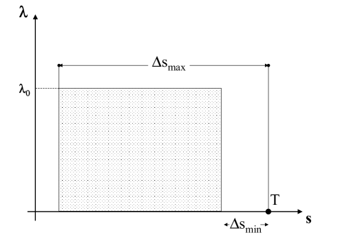
Figure 4: Schematic of the test electron T and the stepped-profile bunch; $\Delta s_{\mathrm{min}}$ indicates the distance between the electron and the head of the bunch; $\Delta s_{\mathrm{max}}$ is the sum of the bunch length and $\Delta s_{\mathrm{min}}$

Now, in order to actually evaluate the transverse electromagnetic force which the bunch exercises on the test particle one has to sum up the contributions from all the retarded sources. Since the two-particle interaction has been calculated in Section II as a function of the retarded angle $\phi$, it is convenient to switch the integration variable from $\Delta s$ to $\phi$,

$${d\Delta s\over{d\phi}}=R\left(1-\beta\cos{\phi\over{2}}\right)$$ (33)

being the Jacobian of the transformation. Therefore, from Eq. (10), Eq. (12) and Eq. (33) one has

$${F_{\mathrm{\bot C}}^{\mathrm{B}}}=\int_{\mathrm{\phi_{\mathrm{min}}}}^{\phi_{\mathrm{max}}}F_{\mathrm{\bot C}}(\phi)~{}R\left(1-\beta\cos(\phi/2)\right)d\phi=$$

$$={e^{2}\lambda_{0}\over{4\pi\varepsilon_{\mathrm{0}}R}}{1\over{2\gamma^{2}}}\left[-{\beta\over{1-\beta\cos(\phi/2)}}-\ln(\tan(\phi/4))\right]_{\mathrm{\phi_{\mathrm{min}}}}^{\phi_{\mathrm{max}}}$$ (35)

and

$${F_{\mathrm{\bot R}}^{\mathrm{B}}}=\int_{\mathrm{\phi_{\mathrm{min}}}}^{\phi_{\mathrm{max}}}F_{\mathrm{\bot R}}(\phi)~{}R\left(1-\beta\cos(\phi/2)\right)d\phi=$$

$$={e^{2}\lambda_{0}\over{4\pi\varepsilon_{\mathrm{0}}R}}\left[\beta^{2}\ln(\tan(\phi/2))+{\beta(1-\beta^{2})\over{1-\beta\cos(\phi/2)}}\right]_{\mathrm{\phi_{\mathrm{min}}}}^{\phi_{\mathrm{max}}} ~{},$$ (37)

where the superscript ”B” stands for ”bunch”, and $\lambda_{0}$ is the constant linear density of the bunch. If we now expand in $\phi_{\mathrm{min}}\ll 1$ and $\phi_{\mathrm{max}}\ll 1$ the trigonometric functions in Eq. (35) and Eq. (37) we have

$${F_{\mathrm{\bot C}}^{\mathrm{B}}}\simeq{e^{2}\lambda_{0}\over{4\pi\varepsilon_{\mathrm{0}}R}}\Bigg{[}-{1\over{\gamma^{2}}}\ln\left({\phi_{\mathrm{max}}\over{\phi_{\mathrm{min}}}}\right)$$

$$-{1\over{2\gamma^{2}}}\left({1\over{1-\beta+\beta\phi_{\mathrm{max}}^{2}/8}}-{1\over{1-\beta+\beta\phi_{\mathrm{min}}^{2}/8}}\right)\Bigg{]}$$ (39)

and

$${F_{\mathrm{\bot R}}^{\mathrm{B}}}\simeq{e^{2}\lambda_{0}\over{4\pi\varepsilon_{\mathrm{0}}R}}\Bigg{[}\ln\left({\phi_{\mathrm{max}}\over{\phi_{\mathrm{min}}}}\right)$$

$$+{1\over{\gamma^{2}}}\left({1\over{1-\beta+\beta\phi_{\mathrm{max}}^{2}/8}}-{1\over{1-\beta+\beta\phi_{\mathrm{min}}^{2}/8}}\right)\Bigg{]} ~{}.$$ (41)

The second term on the right side of Eq. (39) is centrifugal, as well as the first one on the right side of Eq. (41). The other ones are centripetal. Note that the logarithmic term in Eq. (39) is unimportant (in the limit of large values for $\gamma$) with respect to the one in Eq. (41), while the second term in Eq. (39) modifies for a factor $1/2$ the analogous centripetal term in Eq. (41). Therefore, the total transverse force on the test electron is given by:

$${F_{\mathrm{\bot}}^{\mathrm{B}}}\simeq{e^{2}\lambda_{0}\over{4\pi\varepsilon_{\mathrm{0}}R}}\left[\ln\left({\hat{\phi}_{\mathrm{max}}\over{\hat{\phi}_{\mathrm{min}}}}\right)+\left({4\over{4+\hat{\phi}_{\mathrm{max}}^{2}}}-{4\over{4+\hat{\phi}_{\mathrm{min}}^{2}}}\right)\right]~{},$$ (42)

which is the sum of a logarithmic centrifugal term and a centripetal term. It is easy to check that Eq. (42) can be also obtained by direct integration of Eq.(17).

A natural assumption is to consider our bunch density such that there are many particles within a distance $R/\gamma^{3}$ which, as it has already been underlined, is the minimal characteristic distance of the system: if the test particle is to be considered at the head of our bunch, then it is straightforward to assume $\Delta s_{\mathrm{min}}\ll R/\gamma^{3}$ which, by means of the retardation condition Eq. (20), gives us back the condition: $\phi_{\mathrm{min}}\ll 1/\gamma$, the non-linear term in $\phi_{\mathrm{min}}$ of Eq. (20) being, in this case, negligible.

Under the latter assumption we can easily investigate the two cases of a short bunch, that is $\phi_{\mathrm{max}}\ll 1/\gamma$ (in which the linear term in $\phi_{\mathrm{max}}$ of Eq. (20) dominates), and of a long bunch, that is $\phi_{\mathrm{max}}\gg 1/\gamma$ (in which the linear term in $\phi_{\mathrm{max}}$ of Eq. (20) is negligible). These two cases correspond, of course, to the asymptotic situations for the two-particle interaction discussed in Section II.

Let us consider first the case $\phi_{\mathrm{max}}\ll 1/\gamma$. Eq. (39), Eq. (41) and Eq. (42), then, read

$${F_{\mathrm{\bot C}}^{\mathrm{B}}}\simeq{e^{2}\lambda_{0}\over{4\pi\varepsilon_{\mathrm{0}}R}}\left[-{1\over{\gamma^{2}}}\ln\left({\hat{\phi}_{\mathrm{max}}\over{\hat{\phi}_{\mathrm{min}}}}\right)+{1\over{4}}\hat{\phi}^{2}_{\mathrm{max}}\right]$$

(43)

$$\simeq{e^{2}\lambda_{0}\over{4\pi\varepsilon_{\mathrm{0}}R}}\left[-{1\over{\gamma^{2}}}\ln\left({\Delta\hat{s}_{\mathrm{max}}\over{\Delta\hat{s}_{\mathrm{min}}}}\right)+\Delta\hat{s}_{\mathrm{max}}^{2}\right]~{},$$ (44)

$${F_{\mathrm{\bot R}}^{\mathrm{B}}}\simeq{e^{2}\lambda_{0}\over{4\pi\varepsilon_{\mathrm{0}}R}}\left[\ln\left({\hat{\phi}_{\mathrm{max}}\over{\hat{\phi}_{\mathrm{min}}}}\right)-{1\over{2}}\hat{\phi}^{2}_{\mathrm{max}}\right]$$

(45)

$$\simeq{e^{2}\lambda_{0}\over{4\pi\varepsilon_{\mathrm{0}}R}}\left[\ln\left({\Delta\hat{s}_{\mathrm{max}}\over{\Delta\hat{s}_{\mathrm{min}}}}\right)-2\Delta\hat{s}_{\mathrm{max}}^{2}\right]$$ (46)

and

$${F_{\mathrm{\bot}}^{\mathrm{B}}}\simeq{e^{2}\lambda_{0}\over{4\pi\varepsilon_{\mathrm{0}}R}}\left[\ln\left({\hat{\phi}_{\mathrm{max}}\over{\hat{\phi}_{\mathrm{min}}}}\right)-{1\over{4}}\hat{\phi}^{2}_{\mathrm{max}}\right]$$

(47)

$$\simeq{e^{2}\lambda_{0}\over{4\pi\varepsilon_{\mathrm{0}}R}}\left[\ln\left({\Delta\hat{s}_{\mathrm{max}}\over{\Delta\hat{s}_{\mathrm{min}}}}\right)-\Delta\hat{s}_{\mathrm{max}}^{2}\right]~{}.$$ (48)

From Eq. (48) we see that the centripetal term tends, asymptotically, to zero as $(\gamma\phi_{\mathrm{max}})^{2}$.

In the case $\phi_{\mathrm{max}}\gg 1/\gamma$, instead, we have

$${F_{\mathrm{\bot C}}^{\mathrm{B}}}\simeq{e^{2}\lambda_{0}\over{4\pi\varepsilon_{\mathrm{0}}R}}\left[-{1\over{\gamma^{2}}}\ln\left({\hat{\phi}_{\mathrm{max}}\over{\hat{\phi}_{\mathrm{min}}}}\right)+1\right]$$

$$\simeq{e^{2}\lambda_{0}\over{4\pi\varepsilon_{\mathrm{0}}R}}\left[-{1\over{\gamma^{2}}}\ln\left({(24\Delta\hat{s}_{\mathrm{max}})^{1/3}\over{\Delta\hat{s}_{\mathrm{min}}}}\right)+1\right] ~{},$$ (50)

$${F_{\mathrm{\bot R}}^{\mathrm{B}}}\simeq{e^{2}\lambda_{0}\over{4\pi\varepsilon_{\mathrm{0}}R}}\left[\ln\left({\hat{\phi}_{\mathrm{max}}\over{\hat{\phi}_{\mathrm{min}}}}\right)-2\right]$$

(51)

$$\simeq{e^{2}\lambda_{0}\over{4\pi\varepsilon_{\mathrm{0}}R}}\left[\ln\left({(24\Delta\hat{s}_{\mathrm{max}})^{1/3}\over{\Delta\hat{s}_{\mathrm{min}}}}\right)-2\right]$$ (52)

and

$${F_{\mathrm{\bot}}^{\mathrm{B}}}\simeq{e^{2}\lambda_{0}\over{4\pi\varepsilon_{\mathrm{0}}R}}\left[\ln\left({\hat{\phi}_{\mathrm{max}}\over{\hat{\phi}_{\mathrm{min}}}}\right)-1\right]$$

(53)

$$\simeq{e^{2}\lambda_{0}\over{4\pi\varepsilon_{\mathrm{0}}R}}\left[\ln\left({(24\Delta\hat{s}_{\mathrm{max}})^{1/3}\over{\Delta\hat{s}_{\mathrm{min}}}}\right)-1\right]~{},$$ (54)

which means that the centripetal term saturates to a constant value in the limit of a long bunch. The case of a coasting beam (which fits our particular case $\hat{\phi}_{\mathrm{max}}\gg 1$) with transverse extent $h\gg R/\gamma^{2}$ has been discussed in literature (see RUI2 , DERBT , STUP ). As already mentioned above, the presence, in the choice of the model made in the latter works, of a non-negligible transverse dimension alters the structure of the retardation condition (with respect to the one given in Eq. (20)), which explains why the centrifugal part of the transverse force scales, in literature, as $\ln(R/h)$. Moreover, again because of the presence of a transverse dimension, the velocity contribution to the transverse force can be discarded giving the same centripetal term which we found from the radiative term only in Eq. (52), that is $-{2e^{2}\lambda_{0}/(4\pi\varepsilon_{\mathrm{0}}R)}$.

Note that, in order to obtain Eq. (52), we had to integrate contributions from $\hat{\phi}\ll 1$ to $\hat{\phi}\gg 1$: we can give a simple explanation for the centripetal constant force term just analyzing Eq. (17) and its asymptotic behaviours. The product of Eq. (17) with the Jacobian (Eq. (33)) of the transformation between $\Delta\hat{s}$ and $\hat{\phi}$ (this product is just the integrand in Eq. (37)) is equal, in the limits for $\hat{\phi}\gg 1$ and $\hat{\phi}\ll 1$, to $1/\hat{\phi}$: then we can conclude that the logarithmic centrifugal term in Eq. (52) (as well as in Eq. (50 and Eq. (54)) takes into account the $1/\hat{\phi}$-behaviour of the transverse force for the two-particle system, while the constant centripetal term brings information about the way in which the transverse force for a two-particle system changes in the intermediate region between the limits $\hat{\phi}\ll 1$ and $\hat{\phi}\gg 1$. Note, however, that there is no physical ground to distinguish between the first (centrifugal) and the second (centripetal) term in Eq. (54): the total force is always centrifugal, and both terms are consequences of the integration of a unique expression for the force between a two-particle system (which, of course, is always centrifugal too).

IV TRANSVERSE INTERACTION BETWEEN TWO ELECTRONS MOVING IN AN ARC OF A CIRCLE

We will now discuss the case of a two-particle system during the passage from a straight path to a circular one and from a circular path to a straight one. The four possible cases are sketched in Fig. 5 for the case in which the test particle is in front of the source.

The case in which both particles are in the bend, depicted in Fig. 5b, has already been discussed in Section II. Moreover, note that the situation in which the source particle is ahead of the test electron can be treated immediately for all three (a, c and d) transient cases in Fig. 5 (of course, with respect to the figure, test and source particle exchange roles) on the basis of Eq. (23). In fact in such a case, we can assume the retarded angle $\phi$ small enough (the test particle ”runs against” the electromagnetic signal) so that the actual trajectory followed by the particles is not essential and one can use Eq. (23) to describe also the transient cases. Now, the important contribution from the source particle comes from the acceleration part of the Lienard-Wiechert fields. Then, within our approximations, the only non-negligible contribution is constant and identical to the one in Eq. (23), and it is present in the situation (again, with the roles of test and source particle inverted) depicted in Fig. 5a only (Fig. 5b is just the steady-state case).

We will discuss more extensively the consequences of this fact in Section V.

Let us now focus on the cases in which the source particle is behind the test particle and, in particular, let us first deal with the case in Fig. 5a; such a situation occurs when the following condition is met (see SALLONG ):

$$\Delta\hat{s}>{\hat{\phi}\over{2}}+{\hat{\phi}^{3}\over{24}}.$$ (55)

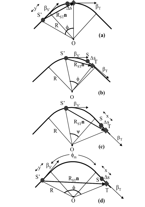
Figure 5: Relative configuration of the retarded source point S’and the test point T for a system of two electron passing a bending magnet.

Let us designate with $y$ the distance, along the straight line before the bend, between the retarded source particle and the beginning of the magnet. The retardation condition, in its approximated form, reads (see SALLONG )

$$\Delta\hat{s}\simeq{\hat{\phi}+\hat{y}\over{2}}+{\hat{\phi}^{3}\over{24}}{\hat{\phi}+4\hat{y}\over{\hat{\phi}+\hat{y}}},$$ (56)

where we introduced the normalized quantity $\hat{y}=y\gamma/R$, which is just $y/R$ normalized to the synchrotron radiation formation angle, $1/\gamma$.

In the situation considered, the source particle is only responsible for a velocity contribution, therefore $F_{\mathrm{\bot}}=F_{\mathrm{\bot C}}$. By direct use of Eq. (8), one can find the exact expression for $F_{\mathrm{\bot}}$

$$F_{\mathrm{\bot}}={e^{2}\over{4\pi\varepsilon_{\mathrm{0}}\gamma^{2}}}{\beta^{2}R(1-\cos\phi)-\beta\sin\phi[(y+R\sin\phi)^{2}+R^{2}(1-\cos\phi)]^{1/2}+R-R\cos\phi+y\sin\phi\over{\left\{[(y+R\sin\phi)^{2}+R^{2}(1-\cos\phi)]^{1/2}-\beta y-R\beta\sin\phi)^{3}\right\}}}$$ (57)

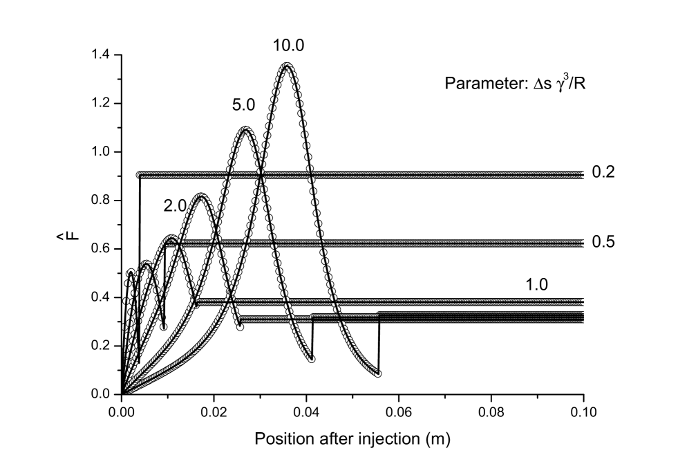
Figure 6: Normalized transverse force ($\hat{F}=F_{\mathrm{\bot}}/[e^{2}/(4\pi\varepsilon_{0}\Delta s)]$) for a two-particle system entering a hard-edge bending magnet as a function of the position after injection. The solid lines show analytical results; the circles describe the outcome from $\mathrm{TRAFIC}^{4}$. We plotted several outcomes from different values of the normalized distance between the two particles.

Expanding the trigonometric functions in Eq. (57) and using normalized quantities one finds:

$$F_{\mathrm{\bot}}\simeq{e^{2}\over{4\pi\varepsilon_{\mathrm{0}}}}{4\gamma^{3}\over{R^{2}}}\hat{\phi}(\hat{y}+\hat{\phi})^{2}$$

(58)

$$\times{\hat{y}^{2}+\hat{y}\left(\hat{\phi}+\hat{\phi}^{3}/2\right)+{\hat{\phi}^{4}/4}\over{\left[(\hat{y}+\hat{\phi})^{2}+{\hat{\phi}^{4}/4}\right]^{3}}}$$ (59)

It can be easily verified that, as it must be, Eq. (59) reduces to Eq. (13) in the limit $y\rightarrow 0$.

It is now possible, by means of Eq. (59), to plot the normalized transverse force $\hat{F}=F_{\mathrm{\bot}}/[e^{2}/(4\pi\varepsilon_{0}\Delta s)]$ as a function of the position after the injection (defined by the entrance of the test particle in the hard-edge magnet) for different values of $\Delta\hat{s}=\Delta s\gamma^{3}/R$. In Fig. 6 we compared such a plot with numerical results from the code $\mathrm{TRAFIC}^{4}$ (see ROTH ).

Note that, at the position which corresponds to the entrance of the retarded source in the magnet there is a discontinuity in the plots. This is linked to our model choice, and it is due to the abrupt (hard edge magnet) switching on of the acceleration fields.

As general remark to Fig. 6 (and to the following ones) it might be worthwhile to stress that the perfect agreement (with graphical accuracy) between our calculations and numerical results by $\mathrm{TRAFIC}^{4}$ provides, per se, an excellent cross-check between analysis and simulations, which enhance one’s level of confidence on both these approaches.

Let us now consider the case depicted in Fig. 5c, in which the source particle has its retarded position inside the bend and the test particle has its present position in the straight line following the magnet. We will define with $x$ the distance, along the straight line after the magnet, between the end of the bend and the present position of the test particle. In this situation the following condition is verified (see SALLONG ):

$$\Delta\hat{s}<{\hat{\phi}_{\mathrm{m}}+\hat{x}\over{2}}+{\hat{\phi}_{\mathrm{m}}^{3}\over{24}}{\hat{\phi}_{\mathrm{m}}+4\hat{x}\over{\hat{\phi}_{\mathrm{m}}+\hat{x}}},$$ (60)

where $\hat{\phi}_{\mathrm{m}}=\gamma\phi_{\mathrm{m}}$, $\phi_{\mathrm{m}}$ being the angular extension of magnet, and $\hat{x}=\gamma x/R$ (the reason for this normalization choice for $x$ is identical to that for $y$) .

The retardation condition reads

$$\Delta\hat{s}\simeq{\hat{\psi}+\hat{x}\over{2}}+{\hat{\psi}^{3}\over{24}}{\hat{\psi}+4\hat{x}\over{\hat{\psi}+\hat{x}}}.$$ (61)

In contrast with the case of Fig. 5a, here we have contributions from both velocity and acceleration field. Again, by direct use of Eq. (8) and Eq. (9) one can find the exact expression for the transverse electromagnetic force performed by the source particle on the test particle

$$F_{\mathrm{\bot}}=F_{\mathrm{\bot C}}+F_{\mathrm{\bot R}}~{},$$ (62)

where

$$F_{\mathrm{\bot C}}={e^{2}\over{4\pi\varepsilon_{\mathrm{0}}\gamma^{2}}}{R(1-\cos\psi)(1-\beta^{2}\cos\psi)-\beta\sin\psi\left[\left((x+R\sin\psi)^{2}+R^{2}(1-\cos\psi)^{2}\right)^{1/2}-\beta x-\beta R\sin\psi\right]\over{\left[\left((x+R\sin\psi)^{2}+R^{2}(1-\cos\psi)^{2}\right)^{1/2}-\beta x\cos\psi-\beta R\sin\psi\right]^{3}}}~{}$$ (63)

and

$$F_{\mathrm{\bot R}}={e^{2}\over{4\pi\varepsilon_{\mathrm{0}}}}{\beta^{2}\over{R}}\Bigg{\{}{-\psi\left[\left((x+R\sin\psi)^{2}+R^{2}(1-\cos\psi)^{2}\right)^{1/2}+\beta x+\beta R\sin\psi\right]-\beta R(1-\cos\psi)\sin\psi\over{\left[\left((x+R\sin\psi)^{2}+R^{2}(1-\cos\psi)^{2}\right)^{1/2}-\beta x\cos\psi-\beta R\sin\psi\right]^{2}}}+$$

$$+{\left(R+x\sin\psi-R\cos\psi\right)\over{\left[\left((x+R\sin\psi)^{2}+R^{2}(1-\cos\psi)^{2}\right)^{1/2}-\beta x\cos\psi-\beta R\sin\psi\right]^{3}}}\times$$

$$\times\Bigg{[}R(1-\cos\psi)(1-\beta^{2}\cos\psi)-\beta\sin\psi\left[\left((x+R\sin\psi)^{2}+R^{2}(1-\cos\psi)^{2}\right)^{1/2}-\beta x-\beta R\sin\psi\right]\Bigg{]}\Bigg{\}}$$ . (66)

Expanding the trigonometric functions in Eq. (63) and Eq. (66), and using normalized quantities one finds:

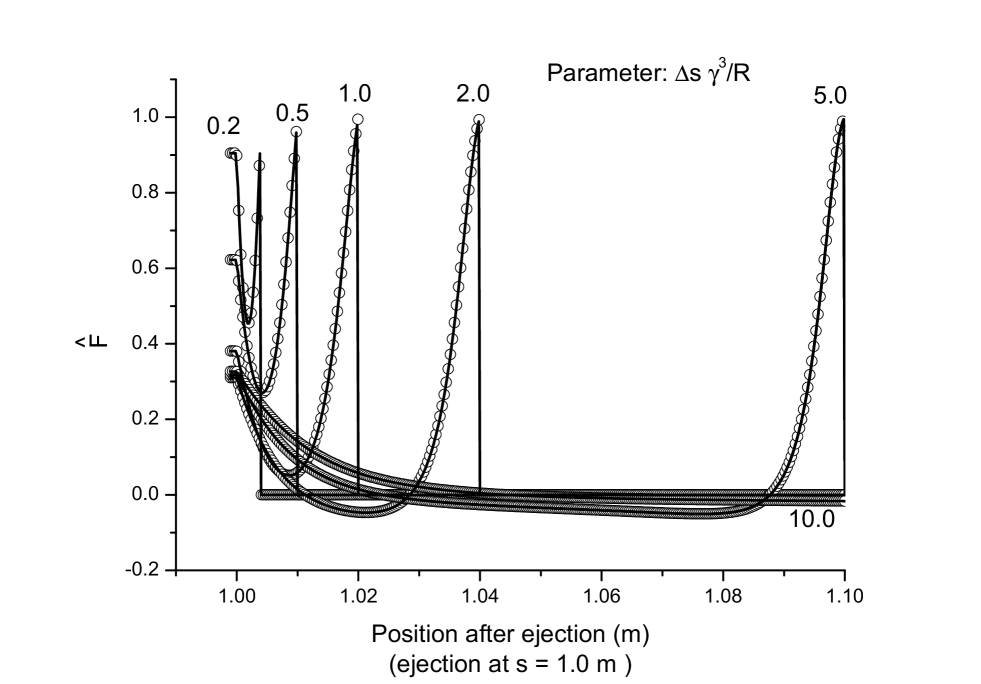
Figure 7: Normalized transverse force ($\hat{F}=F_{\mathrm{\bot}}/[e^{2}/(4\pi\varepsilon_{0}\Delta s)]$) for a two-particle system leaving a hard-edge bending magnet as a function of the position after the ejection. The solid lines show analytical results; the circles describe the outcome from $\mathrm{TRAFIC}^{4}$. We plotted several outcomes from different values of the normalized distance between the two particles.

$$F_{\mathrm{\bot C}}={2e^{2}\gamma^{3}\over{4\pi\varepsilon_{\mathrm{0}}R^{2}}}\hat{\psi}(\hat{x}+\hat{\psi})^{2}{-2\hat{x}^{2}+\hat{x}\left(\hat{\psi}^{3}-2\hat{\psi}\right)+{\hat{\psi}^{4}/2}\over{\left[(\hat{x}+\hat{\psi})^{2}+({\hat{\psi}^{2}/4})(2\hat{x}+\hat{\psi})^{2}\right]^{3}}}~{},$$ (67)

and

$$F_{\mathrm{\bot R}}={2e^{2}\gamma^{3}\over{4\pi\varepsilon_{\mathrm{0}}R^{2}}}(\hat{x}+\hat{\psi})\left\{{\hat{x}^{2}+\hat{x}\hat{\psi}(2-\hat{\psi}^{2})+\hat{\psi}^{2}-3/4\hat{\psi}^{4}\over{\left[(\hat{x}+\hat{\psi})^{2}+(\hat{\psi}^{2}/4)(2\hat{x}+\hat{\psi})^{2}\right]^{2}}}+{(\hat{x}+\hat{\psi})(\hat{x}+{\hat{\psi}/2})\hat{\psi}^{2}\left[-2\hat{x}^{2}+\hat{x}\hat{\psi}(-2+\hat{\psi}^{2})+{\hat{\psi}^{4}/2}\right]\over{\left[(\hat{x}+\hat{\psi})^{2}+(\hat{\psi}^{2}/4)(2\hat{x}+\hat{\psi})^{2}\right]^{3}}}\right\}~{}.$$ (68)

Similarly to the latter case, it can be easily verified that Eq. (67) and Eq. (68) reduce to Eq. (13) and Eq. (14), respectively, in the limit $x\rightarrow 0$. Again, it is possible to plot the normalized transverse force $\hat{F}$ (defined above) as a function of the position after the ejection (defined by the exit of the test particle from the hard-edge magnet) for different values of $\Delta\hat{s}=\Delta s\gamma^{3}/R$. In Fig. 7 we compared such a plot with numerical results from $\mathrm{TRAFIC}^{4}$.

Again, at the position which corresponds to the exit of the retarded source from the magnet there is a discontinuity in the plots. This, again, is linked to our model choice, and it is due to the fact that, for particles on axis, when the retarded source leaves the magnet there is only Coulomb repulsion along the longitudinal direction.

The last case left to discuss is depicted in Fig. 5d; the source particle has its retarded position in the straight line before the bend, and the test particle has its present position in the straight line following the magnet. This case occurs when

$$\Delta\hat{s}>{\hat{\phi}_{\mathrm{m}}+\hat{x}\over{2}}+{\hat{\phi}_{\mathrm{m}}^{3}\over{24}}{\hat{\phi}_{\mathrm{m}}+4\hat{x}\over{\hat{\phi}_{\mathrm{m}}+\hat{x}}}.$$ (69)

The retardation condition reads

$$\Delta\hat{s}\simeq{\hat{\phi}_{\mathrm{m}}+\hat{x}+\hat{y}\over{2}}+{\hat{\phi}_{\mathrm{m}}^{3}\over{24}}{\hat{\phi}_{\mathrm{m}}+4\hat{\phi}_{\mathrm{m}}(\hat{x}+\hat{y})\over{\hat{\phi}_{\mathrm{m}}+\hat{x}+\hat{y}}}.$$ (70)

In this case we have only velocity contributions. The exact expression for the electromagnetic transverse force on the test particle is

$$F_{\mathrm{\bot}}={e^{2}\over{4\pi\varepsilon_{\mathrm{0}}\gamma^{2}}}\Big{\{}(R+y\sin\phi_{\mathrm{m}}-R\cos\phi_{\mathrm{m}})(1-\beta^{2}\cos\phi_{\mathrm{m}})-\beta\sin\phi_{\mathrm{m}}\Big{[}\big{(}2R^{2}+x^{2}+y^{2}+\cos\phi_{\mathrm{m}}(2xy-2R^{2})$$

(71)

$$+2R(x+y)\sin\phi_{\mathrm{m}}\big{)}^{1/2}-\beta(x+y\cos\phi_{\mathrm{m}}+R\sin\phi_{\mathrm{m}})\Big{]}\Big{\}}\Big{\{}\left[2R^{2}+x^{2}+y^{2}+2\cos\phi_{\mathrm{m}}(xy-R^{2})+2R(x+y)\sin\phi_{\mathrm{m}}\right]^{1/2}$$

(72)

$$-\beta\cos\phi_{\mathrm{m}}(x+y\cos\phi_{\mathrm{m}}+R\sin\phi_{\mathrm{m}})-\beta\sin\phi_{\mathrm{m}}(R+y\sin\phi_{\mathrm{m}}-R\cos\phi_{\mathrm{m}})\Big{\}}^{-3}~{}.$$ (73)

Expanding the trigonometric functions in Eq. (73) and using normalized quantities one finds the following approximated expression for $F_{\mathrm{\bot}}$:

$$F_{\mathrm{\bot}}\simeq{e^{2}\over{4\pi\varepsilon_{\mathrm{0}}R^{2}}}8\gamma^{3}(\hat{x}+\hat{y}+\hat{\phi_{\mathrm{m}}})^{2}\phi_{\mathrm{m}}\left\{-{\hat{x}^{2}/2}+{\hat{y}^{2}/2}+({\hat{\phi}_{\mathrm{m}}^{2}/2})\hat{x}\hat{y}+{\hat{x}(\hat{\phi}_{\mathrm{m}}^{3}/4-\hat{\phi}_{\mathrm{m}}/2)}+{\hat{y}(\hat{\phi}_{\mathrm{m}}^{3}/4+\hat{\phi}_{\mathrm{m}}/2)}+{\hat{\phi}_{\mathrm{m}}^{4}/8}\right\}$$

(74)

$$\times{\left\{(\hat{x}+\hat{y}+\hat{\phi}_{\mathrm{m}})\left[\hat{x}(1+\hat{\phi}^{2}_{\mathrm{m}})+\hat{y}+\hat{\phi}_{\mathrm{m}}+{\hat{\phi}^{3}_{\mathrm{m}}/3}\right]-(\hat{\phi}^{2}_{\mathrm{m}}/12)[12\hat{x}\hat{y}+4(\hat{x}+\hat{y})\hat{\phi}_{\mathrm{m}}+\hat{\phi}_{\mathrm{m}}^{2}]\right\}^{-3}}~{}.$$ (75)

It is easy to verify that Eq. (75) reduces, respectively, to the steady state (Eq. (39)) when $x=0$ and $y=0$, to the transient case in Fig. 5a when $x=0$ (Eq. (59)) and to the transient case in Fig. 5d when $y=0$ (Eq. (63)). Following the treatment of the transient situations in Fig. 5a and in Fig. 5c it is possible to plot, for this case too, a normalized expression for the transient force, i.e. the usual $\hat{F}$, as a function of the curvilinear position of the test particle (s=0 indicates the entrance of the magnet) for different values of $\Delta\hat{s}=\Delta s\gamma^{3}/R$ and for different magnet lengths. In Fig. 8, Fig. 9 and Fig. 10 we compared our analytical results with numerical results from $\mathrm{TRAFIC}^{4}$, for the cases $\Delta\hat{s}=0.2$, $\Delta\hat{s}=1.0$ and $\Delta\hat{s}=5.0$ respectively.

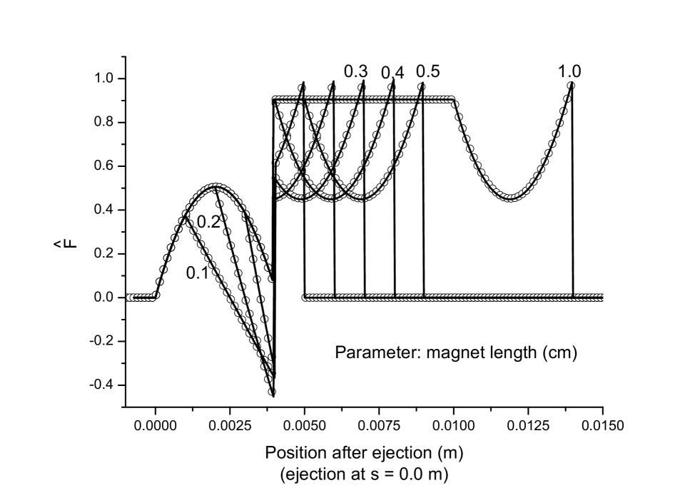
Figure 8: Normalized transverse force ($\hat{F}=F_{\mathrm{\bot}}/[e^{2}/(4\pi\varepsilon_{0}\Delta s)]$) for a two-particle system crossing a hard-edge bending magnet as a function of the position of the test particle inside the magnet in the case of a short magnet $\hat{\phi}_{\mathrm{m}}\ll 1$. The solid lines show analytical results; the circles describe the outcome from $\mathrm{TRAFIC}^{4}$. Here the normalized distance between the two particles is $\Delta\hat{s}=0.2$. We plotted several outcomes from different values of the magnet length $R\hat{\phi}_{\mathrm{m}}=0.1,~{}0.2,~{}0.3,~{}0.4,~{}0.5,~{}1.0$.

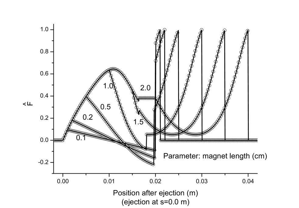
Figure 9: Normalized transverse force ($\hat{F}=F_{\mathrm{\bot}}/[e^{2}/(4\pi\varepsilon_{0}\Delta s)]$) for a two-particle system crossing a hard-edge bending magnet as a function of the position of the test particle inside the magnet in the case of a short magnet $\hat{\phi}_{\mathrm{m}}\ll 1$. The solid lines show analytical results; the circles describe the outcome from $\mathrm{TRAFIC}^{4}$. Here the normalized distance between the two particles is $\Delta\hat{s}=1.0$. We plotted several outcomes from different values of the magnet length $R\hat{\phi}_{\mathrm{m}}=0.1,~{}0.2,~{}0.5,~{}1.0,~{}1.5,~{}2.0$.

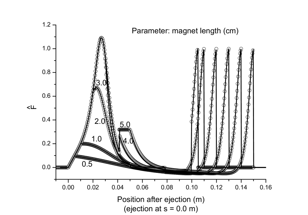
Figure 10: Normalized transverse force ($\hat{F}=F_{\mathrm{\bot}}/[e^{2}/(4\pi\varepsilon_{0}\Delta s)]$) for a two-particle system crossing a hard-edge bending magnet as a function of the position of the test particle inside the magnet in the case of a short magnet $\hat{\phi}_{\mathrm{m}}\ll 1$.The solid lines show analytical results; the circles describe the outcome from $\mathrm{TRAFIC}^{4}$. Here the normalized distance between the two particles is $\Delta\hat{s}=5.0$. We plotted several outcomes from different values of the magnet length $R\hat{\phi}_{\mathrm{m}}=0.5,~{}1.0,~{}2.0,~{}3.0,~{}4.0,~{}5.0$.

V TRANSVERSE INTERACTION BETWEEN AN ELECTRON AND A BUNCH ENTERING A BEND FROM A STRAIGHT PATH

In the previous Section we dealt with all the possible configurations for a two-particle system moving in an arc of a circle. Now, one can consider a bunch moving on the same trajectory and calculate the transverse force on a test particle as the sum of contributions from all the source particles within the bunch.

As an example, we will study here the case of a bunch entering a long bending magnet. Such a case is important, as mentioned before, for code benchmark purposes and for direct application in restricted regions of parameters (negligible transverse bunch size and bunch energy spread).

First we will analyze the case of a bunch with rectangular density function, and we will assume the test particle to be behind the bunch. Such an analysis will be performed using our line model and it is therefore valid only for transverse dimension of the bunch much smaller than the distance between the test particle and the bunch $\Delta s_{\mathrm{min}}$. After the discussion, in Section IV, about a two-particle system with the test particle behind the source electron, one is led to conclude that, within an electron bunch, interactions between sources in front of the test particle and the test particle itself are important and, in general, they must be responsible, at the entrance and at the exit of the bending magnet, for sharp changes in the transverse forces acting on the test electron. The quantitative change depends, of course, on the position of the test particle inside the bunch: the extreme cases are for the test particle at the head of the bunch, where there are just interactions with electrons behind the test particle (no head-tail interactions), and for the test particle at the tail of the bunch, where all the sources are in front of it (only head-tail interactions). It may be worthwhile to underline that the sharp jumps in the transverse force are expected to take place in a space interval comparable, at most, with half of the bunch length, in the case of the test electron at the tail of the bunch. In order to show this, one can easily calculate the transverse force acting on a test particle behind a bunch with rectangular density distribution entering a hard-edge magnet. If, as usual, we indicate with $\Delta s_{\mathrm{max}}$ the distance from the test particle to the head of the bunch and with $\Delta s_{\mathrm{min}}$ the distance from the test particle to the tail of the bunch, then one can easily derive such an expression from Eq. (22) and Eq. (23):

$${F_{\mathrm{\bot~{}HT}}^{\mathrm{B}}}(\phi)\simeq\Bigg{\{}\begin{array}[]{c}0~{}~{}~{}~{}~{}~{}~{}~{}~{}~{}~{}~{}~{}~{}~{}~{}~{}~{}~{}~{}~{}~{}~{}~{}~{}~{}~{}~{}~{}~{}~{}~{}~{}~{}~{}~{}~{}~{}~{}\phi<0\\ e^{2}\lambda_{0}/(4\pi\varepsilon_{\mathrm{0}}R)~{}\ln\left[\Delta s_{\mathrm{max}}/(\Delta s_{\mathrm{max}}-R\phi(1+\beta))\right]~{}~{}~{}~{}~{}~{}~{}~{}0<\phi<(\Delta s_{\mathrm{max}}-\Delta s_{\mathrm{min}})/[R(1+\beta)]\\ e^{2}\lambda_{0}/(4\pi\varepsilon_{\mathrm{0}}R)~{}\ln[\Delta s_{\mathrm{max}}/\Delta s_{\mathrm{min}}]~{}~{}~{}~{}~{}~{}~{}~{}~{}~{}~{}~{}~{}~{}~{}~{}~{}~{}~{}~{}~{}~{}~{}~{}~{}~{}~{}~{}~{}~{}~{}~{}~{}~{}\phi>(\Delta s_{\mathrm{max}}-\Delta s_{\mathrm{min}})/[R(1+\beta)]\end{array}~{},$$ (76)

where ”HT” stands for ”head-tail”.

The following step is to actually plot the transverse force in Eq. (76). It is convenient to choose, as normalization factor for the transverse force, the value $f_{1}={e^{2}\lambda_{0}/(4\pi\varepsilon_{\mathrm{0}}R)}\ln[\Delta s_{\mathrm{max}}/\Delta s_{\mathrm{min}}]$. Our results, compared, once again, with simulations by $\mathrm{TRAFIC}^{4}$, are shown in Fig. 11 for a bunch length $\Delta s_{\mathrm{max}}-\Delta s_{\mathrm{min}}=100~{}\mu$m, $\gamma=100$, $R=1$ m and for $\Delta s_{\mathrm{min}}=1~{}\mu$m. This means that, according to the validity limits of our model, this result can be applied only when $h\ll 1~{}\mu$m. Nevertheless, this simple example shows that the code TRAFIC⁴ is actually able to account for head-tail interactions. Note that, as expected, the transient has a spatial extent of about one half of the bunch length ($\Delta s_{\mathrm{max}}/(1+\beta)$).

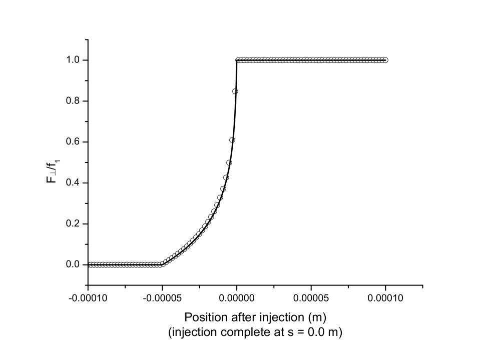
Figure 11: Normalized transverse force $F_{\mathrm{\bot}}/f_{1}$ acting on a test particle behind a bunch with rectangular density distribution. As the bunch enters a hard-edge bending magnet we plot the normalized force as a function of the position of the test particle inside the magnet (solid line) and we compare with results by $\mathrm{TRAFIC}^{4}$ (circles). Parameters choice are: bunch length $=100\mu m$, $\gamma=100$, $R=1m$; the value of $\Delta s_{\mathrm{min}}$ is $1\mu$m.

We will now analyze the case of a bunch with rectangular density function with the test particle in front of the bunch, as depicted in Fig. 4. In the injection case we have contributions from retarded sources both in the bend and in the straight line before the bend. The contribution from the retarded sources in the magnet is given, basically, by Eq. (42), and reads

$${F_{\mathrm{\bot m}}^{\mathrm{B}}}\simeq{e^{2}\lambda_{0}\over{4\pi\varepsilon_{\mathrm{0}}R}}\left[\ln\left({\hat{\phi}_{\mathrm{max}}\over{\hat{\phi}_{\mathrm{min}}}}\right)+{4\over{4+\hat{\phi}^{2}_{\mathrm{max}}}}-{4\over{4+\hat{\phi}^{2}_{\mathrm{min}}}}\right]~{},$$ (77)

where ”m” reminds that the contributions treated by Eq. (77) are all from the ”magnet”. All that is left to do now, is the investigation of the values which $\hat{\phi}_{\mathrm{min}}$ and $\hat{\phi}_{\mathrm{max}}$ assume. Let us first define with $\hat{\phi}^{*}$ the solution of the retardation equation $\Delta\hat{s}_{\mathrm{min}}=\hat{\phi}^{*}/2+\hat{\phi}^{*3}/24$. If $\hat{\phi}^{*}<\hat{\phi}$, the retarded position of the first source particle is in the bending magnet, and $\hat{\phi}_{\mathrm{min}}=\hat{\phi}^{*}$. On the other hand, when $\hat{\phi}^{*}>\hat{\phi}$ there are no contributions to the transverse force from the bend. Next, we define with $\hat{\phi}^{**}$ the solution of $\Delta\hat{s}_{\mathrm{max}}=\hat{\phi}^{**}/2+\hat{\phi}^{**3}/24$. Supposing $\hat{\phi}^{*}<\hat{\phi}$, if $\hat{\phi}^{**}<\hat{\phi}$ too, then all the particles contribute from the bend, and $\hat{\phi}_{\mathrm{max}}=\hat{\phi}^{**}$. On the other hand, when $\hat{\phi}^{**}>\hat{\phi}$, we have a mixed situation, in which part of the particles contribute from the bend and others from the straight line before the magnet. In this case $\hat{\phi}_{\mathrm{max}}=\hat{\phi}$.

The contribution from the retarded sources in the straight path before the bend is given by

$${F_{\mathrm{\bot s}}^{\mathrm{B}}}=\int_{\mathrm{\Delta\hat{s}_{\mathrm{min}}}}^{\Delta\hat{s}_{\mathrm{max}}}{R\over{\gamma^{3}}}F_{\mathrm{\bot}}(\hat{y}(\Delta\hat{s}),\hat{\phi})d\Delta\hat{s}~{},$$ (78)

where ”s” stands for ”straight path”, and where the expression for $F_{\mathrm{\bot}}$ in the integrand is given by Eq. (59). It is convenient, as done before, to switch the integration variable from $\Delta\hat{s}$ to $\hat{y}$. The Jacobian of the transformation is given by (see SALLONG )

$${d\Delta\hat{s}\over{d\hat{y}}}\simeq{(\hat{\phi}+\hat{y})^{2}+\hat{\phi}^{4}/4\over{2(\hat{\phi}+\hat{y})^{2}}}$$ (79)

After substitution of Eq. (79) and Eq. (59) in Eq. (78), one can easily carry out the integration, thus getting

$${F_{\mathrm{\bot\mathrm{s}}}^{\mathrm{B}}}\simeq{2e^{2}\lambda_{0}\over{4\pi\varepsilon_{\mathrm{0}}R}}\Bigg{[}{\hat{\phi}\left(4\hat{y}_{\mathrm{min}}+2\hat{\phi}+\hat{\phi}^{3}\right)\over{4\hat{y}_{\mathrm{min}}^{2}+8\hat{y}_{\mathrm{min}}\hat{\phi}+4\hat{\phi}^{2}+\hat{\phi}^{4}}}$$

$$-{\hat{\phi}\left(4\hat{y}_{\mathrm{max}}+2\hat{\phi}+\hat{\phi}^{3}\right)\over{4\hat{y}_{\mathrm{max}}^{2}+8\hat{y}_{\mathrm{max}}\hat{\phi}+4\hat{\phi}^{2}+\hat{\phi}^{4}}}\Bigg{]} ~{}.$$ (81)

As done before for $\hat{\phi}_{\mathrm{min}}$ and $\hat{\phi}_{\mathrm{max}}$, we can now investigate the values of $\hat{y}_{\mathrm{min}}$ and $\hat{y}_{\mathrm{max}}$. Let us start with $\hat{y}_{\mathrm{min}}$. First, we define with $\hat{y}^{*}$ the solution of the retardation condition $\Delta\hat{s}_{\mathrm{min}}=(\hat{\phi}+\hat{y}^{*})/2+(\hat{\phi}^{*3}/24)(4\hat{y}^{*}+\hat{\phi})/({\hat{y}^{*}+\hat{\phi}})$. If $\hat{y}^{*}>0$, the retarded position of the first source particle is in the straight line before bending magnet, and $\hat{y}_{\mathrm{min}}=\hat{y}^{*}$. On the other hand, when $\hat{y}^{*}<0$, the retarded position of the first source particle is in the bend, and $\hat{y}_{\mathrm{min}}=0$.

Next, we define with $\hat{y}^{**}$ the solution of $\Delta\hat{s}_{\mathrm{max}}=(\hat{\phi}+\hat{y}^{*})/2+(\hat{\phi}^{*3}/24)(4\hat{y}^{*}+\hat{\phi})/({\hat{y}^{*}+\hat{\phi}})$. Consider the case $\hat{y}^{**}<0$: all the particles contribute from the bend, that is we entered the steady-state situation. In this case $\hat{y}_{\mathrm{max}}=\hat{y}_{\mathrm{min}}=0$. On the other hand, when $\hat{y}^{**}>0$, we have again a mixed situation, in which part of the particles contribute from the bend and others from the straight line before the magnet. In this case $\hat{y}_{\mathrm{max}}=\hat{y}^{**}$.

The following step is to actually plot the transverse force on an electron from a bunch with rectangular distribution entering a long bend. It is convenient to choose, as normalization factor for the transverse force, the value $f={e^{2}\lambda_{0}/(4\pi\varepsilon_{\mathrm{0}}R)}\ln(\Delta\hat{s}_{\mathrm{max}})$. Our results, compared, once again, with simulations by $\mathrm{TRAFIC}^{4}$, are shown in Fig. 12 for a bunch length of $100~{}\mu$m, $\gamma=100$, $R=1$ m and for different values of $\Delta\hat{s}$.

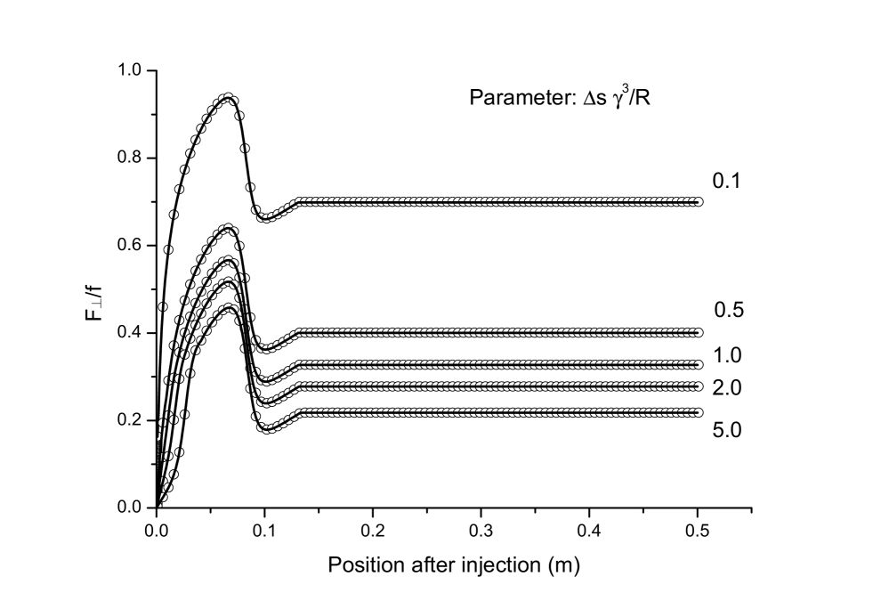
Figure 12: Normalized transverse force ($F_{\mathrm{\bot}}/f$) acting on a test particle from a bunch with rectangular density distribution entering a hard-edge bending magnet as a function of the position of the test particle inside the magnet. The solid lines show analytical results; the circles describe the outcome from $\mathrm{TRAFIC}^{4}$. We chose $\Delta s_{\mathrm{max}}=100\mu$m, $\gamma=100$, $R=1$ m; graphs are plotted for several values of the parameter $\Delta\hat{s}_{\mathrm{min}}$.

It is interesting to calculate the asymptotic expression for $F^{\mathrm{B}}_{\mathrm{\bot s}}$ in the limit for a long bunch ($\Delta\hat{s}_{\mathrm{max}}\gg 1$) and for a short distance between the test particle and the head of the bunch ($\Delta\hat{s}_{\mathrm{min}}\ll 1$). First let us indicate with $\hat{\phi}_{\mathrm{b}}$ the normalized angular extension of the bunch ($\hat{\phi}_{\mathrm{b}}=\gamma\phi_{\mathrm{b}}$, where $\phi_{\mathrm{b}}$ is just the ratio between the bunch length and the radius of the circle $R$). By means Eq. (56) it is easy to prove that, when $\hat{\phi}/\hat{\phi}_{\mathrm{b}}<2^{-2/3}$, $\hat{y}_{\mathrm{max}}$ takes bigger and bigger values, with an upper limit $\hat{y}_{\mathrm{max}}=2\Delta\hat{s}_{\mathrm{max}}$. On the other hand, when $\hat{\phi}/\hat{\phi}_{\mathrm{b}}>2^{-2/3}$, $\hat{y}_{\mathrm{max}}$ takes always decreasing values, with a lower limit $\hat{y}_{\mathrm{max}}=0$. Assuming $\hat{y}_{\mathrm{min}}\ll 1$, one may check that, in the long bunch limit, Eq. (81) reads

$$F^{\mathrm{B}}_{\mathrm{\bot s}}\simeq\Bigg{\{}\begin{array}[]{c}{e^{2}\lambda_{0}/(2\pi\varepsilon_{\mathrm{0}}R)}~{}~{}~{}~{}~{}~{}\hat{\phi}/\hat{\phi}_{\mathrm{b}}<2^{-2/3}\\ 0~{}~{}~{}~{}~{}~{}~{}~{}~{}~{}~{}~{}~{}~{}~{}~{}~{}~{}~{}~{}~{}~{}~{}\hat{\phi}/\hat{\phi}_{\mathrm{b}}>2^{-2/3}\end{array}~{},$$ (82)

which is a boxcar function. Note that in the passage from Eq. (81) to Eq. (82) we used the fact that $\hat{\phi}\gg 1$. In order to visualize the limiting process we plotted, in Fig. 13, $F^{\mathrm{B}}_{\mathrm{\bot s}}$, as it is given in Eq. (81) and normalized to $f={e^{2}\lambda_{0}/(4\pi\varepsilon_{\mathrm{0}}R)}\ln(\Delta\hat{s}_{\mathrm{max}})$ (i.e. $v=F^{\mathrm{B}}_{\mathrm{\bot s}}/f$, in the plot), as a function of the position after injection, normalized to $\hat{\phi}_{\mathrm{b}}$ (i.e. $u=R\hat{\phi}/(\gamma\hat{\phi}_{\mathrm{b}})$, in the plot). The plots in Fig. 13a, b, c and d refer to different bunch lengths (respectively $10^{2}\mu$m, $10^{3}\mu$m, $10^{4}\mu$m and $10^{5}\mu$m). For every choice of the bunch length we show different outcomes for several choices of $\Delta\hat{s}_{\mathrm{min}}$. As one can see from Fig. 13, in the limit for $\Delta\hat{s}_{\mathrm{min}}\ll 1$ and $\Delta\hat{s}_{\mathrm{max}}\gg 1$, one approaches the boxcar function described by Eq. (82). Note that, here, the radius of the bend is $R=1$m and $\gamma=100$, therefore we have $2^{-2/3}R/\gamma\simeq 6.3\cdot 10^{-3}$m, while the maximum value for $v$, due to the normalization choice, is given, from Eq. (82), by $2/\ln(\hat{\Delta}s_{\mathrm{min}})$. In the case of Fig. 13d, for example, we have $2/\ln(\Delta\hat{s}_{\mathrm{min}})\simeq 0.174$ (in agreement, of course, with the maximum value found in the plot).

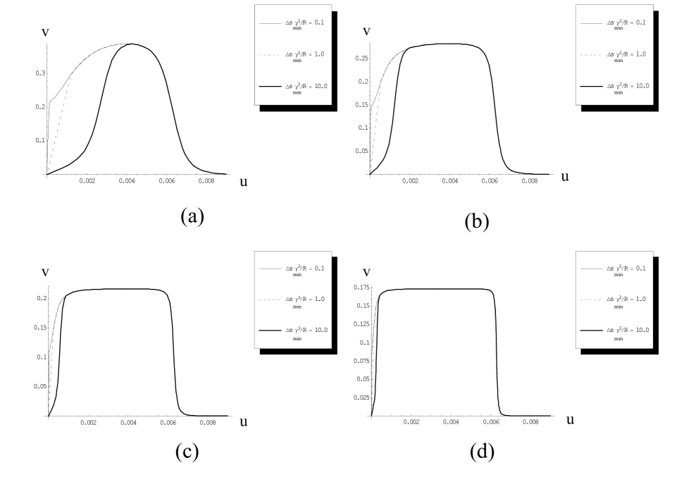
Figure 13: Plot of $v=F^{\mathrm{B}}_{\mathrm{\bot s}}/f$ as a function of $u=R\hat{\phi}/(\gamma\hat{\phi}_{\mathrm{b}})$; here $R=1$m and $\gamma=100$. Case (a) the bunch length is $10^{2}\mu$m, (b) $10^{3}\mu$m, (c) $10^{4}\mu$m and (d) $10^{5}\mu$m. Each case is parameterized with respect to different values of $\Delta\hat{s}_{\mathrm{min}}=\gamma^{3}\Delta s_{\mathrm{min}}/R$ (see the legends in the plots).

On the other hand, again in the same limits, one can find the asymptotic expression for the contribution from particles with retarded position in the bend: this is given, indeed, by Eq. (77), with the limit expressions for $\hat{\phi}_{\mathrm{min}}$ in the case of a small distance $\Delta\hat{s}_{\mathrm{min}}$, and $\hat{\phi}_{\mathrm{max}}$ in the long bunch limit. For $\hat{\phi}_{\mathrm{min}}$ we have, from the retardation condition in Eq. (56) $\hat{\phi}_{\mathrm{min}}=2\hat{s}_{\mathrm{min}}$.

For $\hat{\phi}_{\mathrm{max}}$, if $\Delta\hat{s}_{\mathrm{max}}<\hat{\phi}^{3}/24$ we have, again from Eq. (56), $\hat{\phi}_{\mathrm{max}}=\hat{\phi}_{\mathrm{b}}=(24\Delta\hat{s}_{\mathrm{max}})^{1/3}$. Otherwise, when $\Delta\hat{s}_{\mathrm{max}}>\hat{\phi}^{3}/24$ then $\hat{\phi}_{\mathrm{max}}=\hat{\phi}$, and we have the steady state situation.

By means of these results one can build an expression for the transverse force in the case of a bunch with general density distribution $\lambda$, by considering it as a composition of rectangular bunches with length $(s-s^{\prime})$ and linear density $ds^{\prime}d\lambda(s^{\prime})/ds^{\prime}$, under the constraint that the important bunches for such a composition are long enough to neglect all linear terms in the expression for the retardation condition (i.e. $\lambda(s)\gamma^{3}/R\gg d\lambda(s^{\prime})/ds^{\prime}$, see SALLONG ). In this case, the contribution from particles in the straight line reads

$${F_{\mathrm{\bot s}}^{\mathrm{tot}}}\simeq\int_{\mathrm{-\infty}}^{s-R\phi^{3}/6}F_{\mathrm{\bot s}}^{\mathrm{B}}(\phi,s-s^{\prime}){d\lambda(s^{\prime})\over{ds^{\prime}}}ds^{\prime}$$

(83)

$$={e^{2}\over{2\pi\varepsilon_{\mathrm{0}}R}}\lambda(s-R\phi^{3}/6)$$ (84)

Note that the latter expression does not depend on $\Delta s_{\mathrm{min}}$. On the other hand the contribution from particles in the bend is

$${F_{\mathrm{\bot m}}^{\mathrm{tot}}}\simeq\int_{\mathrm{-\infty}}^{s-s_{\mathrm{min}}}F_{\mathrm{\bot m}}^{\mathrm{B}}(\phi,s-s^{\prime}){d\lambda(s^{\prime})\over{ds^{\prime}}}ds^{\prime}$$

(85)

$$={e^{2}\over{2\pi\varepsilon_{\mathrm{0}}R}}\int_{\mathrm{-\infty}}^{s-s_{\mathrm{min}}}{1\over{2}}\Bigg{[}-1+{1\over{3}}\ln\left({24\gamma^{3}\over{R}}{\Delta s}_{\mathrm{max}}\right)$$

(86)

$$-\ln\left({2\gamma^{3}\over{R}}{\Delta s}_{\mathrm{min}}\right)\Bigg{]}{d\lambda(s^{\prime})\over{ds^{\prime}}}ds^{\prime}~{},$$ (87)

which, instead, depends on $\Delta s_{\mathrm{min}}$. It is very interesting to show that this dependence on $\Delta s_{\mathrm{min}}$ cancels with the dependence on $\Delta s_{\mathrm{min}}$ of the steady-state force: in fact this constitutes a general result independent from the choice of the position of the test particle. In order to show this, let us first note that Eq. (87) can be written as

$${F_{\mathrm{\bot m}}^{\mathrm{tot}}}\simeq{e^{2}\over{4\pi\varepsilon_{\mathrm{0}}R}}\times$$

$$\times\Bigg{\{}\int_{\mathrm{s-\phi^{3}R/24}}^{s-s_{\mathrm{min}}}\left[-1+\ln(\hat{\phi}_{\mathrm{b}}(s^{\prime}))-\ln(\hat{\phi}_{\mathrm{min}})\right]{d\lambda(s^{\prime})\over{ds^{\prime}}}ds^{\prime}+$$

$$+\int_{\mathrm{-\infty}}^{s-\phi^{3}R/24}\left[-1+\ln(\hat{\phi})-\ln(\hat{\phi}_{\mathrm{min}})\right]{d\lambda(s^{\prime})\over{ds^{\prime}}}ds^{\prime}\Bigg{\}} ~{},$$ (90)

while the steady state contribution is given by

$${F_{\mathrm{\bot steady}}^{\mathrm{tot}}}\simeq{e^{2}\over{4\pi\varepsilon_{\mathrm{0}}R}}\times$$

(91)

$$\times\int_{\mathrm{-\infty}}^{s-s_{\mathrm{min}}}\left[-1+\ln(\hat{\phi}_{\mathrm{b}}(s^{\prime}))-\ln(\hat{\phi}_{\mathrm{min}})\right]{d\lambda(s^{\prime})\over{ds^{\prime}}}ds^{\prime}~{}.$$ (92)

Subtracting side by side Eq. (92) from Eq. (90), and adding the contribution from the straight path, one finally gets the following ”regularized” expression for the transient transverse force:

$${\widetilde{F}_{\mathrm{\bot}}^{\mathrm{tot}}}\simeq{e^{2}\over{2\pi\varepsilon_{\mathrm{0}}R}}\Bigg{[}\lambda(s-R\phi^{3}/6)-$$

(93)

$$-{1\over{6}}\int_{\mathrm{-\infty}}^{s-R\phi^{3}/24}\ln\left(24(s-s^{\prime})\over{R\phi^{3}}\right){d\lambda(s^{\prime})\over{ds^{\prime}}}ds^{\prime}\Bigg{]}~{},$$ (94)

which is completely independent from $\Delta s_{\mathrm{min}}$ and, therefore, free from singularity in the limit $\Delta s_{\mathrm{min}}\rightarrow 0$. It might be worthwhile to remark that usual regularization techniques take place, in the study of longitudinal (CSR) self-interactions (see SALLONG ) at the stage of the two-particle system and before integration of the contributions from all the retarded sources within the bunch. The situation is reversed here, where regularization takes place after integration.

VI TRANSVERSE DYNAMICS AND CANCELLATION OF CENTRIFUGAL FORCES

We will discuss here, from a qualitative viewpoint, the effect of perpendicular forces on the transverse beam dynamics (although, as we stated in Section I, this article is mainly devoted to the study of electrodynamical effects). In particular we will concentrate on the controversial issue of the cancellation of the centrifugal force, in the transverse equation of motion of a particle, by the ratio between the electron energy deviation of from its nominal value and the design radius $R$ (see RUI2 , LEE … STUP , LCLS ).

To illustrate this cancellation as it is explained in literature, let us consider a bunch moving in a circular orbit with design radius $R$, and let us indicate with $X$ the transverse displacement of a test electron from the equilibrium orbit. Then (see, for example, RUI2 ), up to the first order in $X$, one can easily write the equation for the transverse motion of the test electron as:

$${d^{2}X\over{c^{2}dt^{2}}}+{X\over{R^{2}}}={\Delta E_{0}\over{RE_{0}}}+{F_{r}\over{E_{0}}},$$ (95)

where $E_{0}=\gamma_{0}mc^{2}$ is the design energy (which is linked to the equilibrium radius by the relation $\beta\gamma_{0}mc=eBR$), $\Delta E_{0}=(\gamma-\gamma_{0})mc^{2}$ is the kinetic energy deviation, from $E_{0}$ and, finally, $F_{r}$ is the self-interaction force in the transverse direction.

We already discussed (see Section III) the fact that the transverse force on a test electron, both on-orbit ($X=0$) and off-orbit ($X\neq 0$) can be written, in the long bunch limit, as the sum of two terms: a logarithmic, centrifugal term, and a constant, centripetal one.

In LCLS , the case of bunch compression by means of a magnetic chicane (at LCLS) is analyzed, and the centrifugal term is told to be essentially (aside for a negligible residual) canceled by part of the $\Delta E_{0}$-term in Eq. (95). In fact all contributions to the transverse emittance growth are attributed to the centripetal force ”which originates from radiation of trailing particles and depends on the local charge density along the bunch. The maximum force takes place at the center of the bunch and its effect on the transverse emittance is estimated in the reference. This estimate predicts an emittance growth of $\ll 1\%$ for the worst case (last dipole of chicane-2 where the bunch is shortest)” (quoted from LCLS ).

Here we will discuss this effect, well known to the CSR community as ”the cancellation effect”, within the limits of our line model, and show that, in contrast to what has been implicitly assumed in LCLS , it has no general validity.

As a general remark to all the previous analysis of the problem, we must say that, up to now, only the situation of sources behind the test particle has been discussed, while we know, from Section IV, that head-tail interactions are present too: they are characterized, at least within the limits of our model, by a magnitude of the same order of the tail-head interactions and the spatial extension of their transient is negligible (comparable, at most, with half of the bunch length). Since this centrifugal force depends on the position of the test particle along the bunch, it will be responsible for normalized emittance growth.

Anyway, let us consider, in particular, the tail-head interaction problem. As underlined in Section I, the full solution to the evolution problem is met when one is able to solve simultaneously the equation of motion and the equation for the electromagnetic field. Then, in principle, we may adopt, in our discussion, two separate viewpoints: in the first one we imagine to solve, in some way, the full evolution problem, while in the second we treat the same situation by means of a perturbation theory approach, assuming that, in first approximation, the motion of a rigid bunch is driven by the external magnetic field alone and then calculating the perturbation to the particle motion due to transverse self-fields: we will show that, in both cases, the cancellation effect has no general validity.

Let us begin with the first viewpoint. Generally speaking, if there was complete compensation between the total transverse force and the $\Delta E_{0}$-term, then the particles with the same total energy (assumed equal to the sum of kinetic energy and potential self-energy from the bunch) would have followed the same trajectory. Such a complete cancellation would be based upon two assumptions. Firstly, $\Delta E_{0}=-e\Delta\Phi$ and, secondly, $F_{\bot}=e\Phi/R$. Note that, in this case, $\Delta E_{0}+RF_{\bot}=e\Phi(0)$. This, of course, is not the case, since the cancellation has always been understood for the centrifugal term alone (and, anyway, it is not complete). Moreover let us remind that, as explained in Section III, there is no physical ground to distinguish between the centripetal term and the centrifugal one: from a physical viewpoint there is just an overall centrifugal force. A further subdivision is just of mathematical nature, and explains how the transverse force plotted in Fig. 2 behaves from one asymptotic (short distance between test and source particle) to the other (large distance between test and source particle). This fact, alone, suggests that the cancellation issue has no general validity and that, indeed, it is artificial (as the subdivision between centripetal and centrifugal term is) even when it works, like in the case of a coasting beam in a simple, circular steady-state motion.

Nevertheless, let us retain, in our terminology, the distinction between centripetal and centrifugal term. Then, a complete cancellation between centrifugal force and potential term would be based, similarly as before, upon two facts. Firstly, $\Delta E_{0}=-e\Delta\Phi$ and, secondly, $F_{\bot}^{\mathrm{centrifugal}}=e\Phi/R$, at any time. Whenever one of these assumptions is no more verified, the cancellation fails to happen.

Of course, in order to show that the cancellation effect is not valid in general, it is sufficient to provide a counter-example. Let us consider, therefore, the case of a bunch with zero initial energy spread or, more simply, a two-particle system with the test electron in front of the source, such that $\Delta\gamma=\gamma-\gamma_{0}=0$. Let us restrict to a case in which only space charge effects are important, as concerns the longitudinal motion: therefore we consider, in this sense, two electrons running on a straight path.

The Coulomb (space-charge) interaction changes both the kinetic energy of the particles and their relative distance, which we will assume, initially, equal to $\Delta s$ in the laboratory frame. Let us deal with the problem in the (instantaneous) rest frame of the center of mass of the system (simply designated as the rest frame, in the following) and assume that the particles do not move relativistically in such a frame. After a long time one will be left, asymptotically, with two particles far away from each other, each one with a kinetic energy equal to $e^{2}/(8\pi\epsilon_{0}\Delta\widetilde{s})$, where $\Delta\widetilde{s}=\gamma\Delta s$. Therefore, the change in kinetic energy of the test particle in the laboratory frame, can be found by means of a Lorentz transformation (performed on the momentum in the longitudinal direction):

$$\Delta E_{0}=\gamma{c\over{\beta}}\left({2me^{2}\over{8\pi\epsilon_{0}\gamma\Delta s}}\right)^{1/2}={c\over{\beta}}\left({\gamma me^{2}\over{4\pi\epsilon_{0}\Delta s}}\right)^{1/2}~{}.$$ (96)

On the other hand, again in the asymptotic limit, the potential energy of the test electron (as well as the one of the source) will approach zero. Then, at least after a long time from the beginning of the evolution, one has

$$\Delta E_{0}(t\rightarrow\infty)\neq-e\Delta\Phi(t\rightarrow\infty)=e\Phi(0)~{}.$$ (97)

This means that the first assumption for the cancellation ($\Delta E_{0}=-e\Delta\Phi$ at every time) is violated, due to the inclusion of space charge forces in the longitudinal motion; as a result we can say that there is no cancellation effect.

Of course, one could also treat the situation of a circular motion, which is more complicated, but the example we gave is sufficient to show that the effect is not valid in general.

We are now left to deal with the second viewpoint. As it has already been said above, by following this approach, we assume that, in zero approximation, the particles move under the action of the external field alone and then, once the particles motion is fixed (in the zeroth order), one can calculate the perturbation to such a motion due to self-fields. Note that, if one treats in this framework the example of a coasting beam or of a rigid line bunch with finite longitudinal dimension, then $\Phi$ is constant, which suggest there are no more contradictions with the cancellation assumptions. Nevertheless we will now show that cancellation is far from being a general effect. Let us study, first, the case of a rigid bunch. Consider, for example, the two cases of a rigid line bunch oriented either along the velocity or perpendicular to it (see Fig. 14).

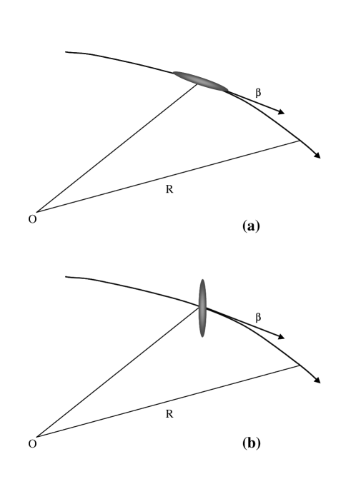
Figure 14: Schematic of a line bunch in a circular trajectory; (a) the line bunch is oriented along the velocity; (b) the line bunch is oriented perpendicularly with respect to the velocity.

For simplicity we can study the non-relativistic case: in the relativistic one we have an analogous situation. The kinetic energy of the line bunch and the scalar potential acting on each particle do not depend on the orientation of the bunch with respect to the velocity vector. If the cancellation effect had general validity, also the transverse self-force should not depend on the orientation but, indeed, one can easily verify that, for the case of the line bunch oriented along the perpendicular direction (see Fig. 14b), the self-interaction force is two times smaller than in the case of orientation along the longitudinal direction. In fact, in the case of the bunch oriented in the longitudinal direction we have repelling forces parallel to the velocity vector while, in the other case, they are perpendicular: according to Eq. (27), the momentum flux along the parallel direction (that is $T_{33}$) is then equal to the potential energy but having opposite sign in the first case, and equal to zero in the second. This fact shows that the cancellation effect has no general validity. This can be discussed in a somewhat deeper way too. As we showed in Section II, in order to get a correct dynamical interpretation of the electrodynamical transverse forces for a two-particle system, one needs to account for the self-interaction energy and momentum flux and, by doing so, the energy and momentum of the system do not form a four-vector anymore (as, instead, people always assume in considering the cancellation issue). They are, indeed, components of a second rank tensor (the energy-momentum tensor) and, therefore, transform in a different way with respect to a four-vector: this is the conceptual reason which explains why the cancellation is not a fundamental effect; as soon as one cannot consider energy and momentum as a four-vector anymore the cancellation is spoiled, in general, by the $T_{33}$ component of the stress tensor in the rest frame.

Also the analysis of the transient behavior leads to the conclusion that the compensation is not of general importance. Let us consider the case of a bunch entering a bend (which we discussed in Section V, in the laboratory frame. The formation length for both the scalar potential and the transverse force (after which the bunch reaches the steady state situation) is simply the overtaking length $2(3sR^{2})^{1/3}$. Now, on the one hand the transverse force is zero at the beginning of the bend, and relaxes to a $\gamma$-independent value in the steady-state situation while, on the other hand, the scalar potential starts from a $\gamma$-dependent value before the bend and relaxes to a $\gamma$-independent value in the steady state regime too. Comparing the two transients for the scalar potential and for the transverse force, we can therefore conclude that the first one is characterized by an additional free parameter (the initial value of the beam energy) with respect to the second, and this means that the two transients are completely independent. As a result, again, the compensation proves to fail in this case (since it should follow from the subtraction of the centrifugal force with the term, in $\Delta E_{0}/(RE_{0})$, proportional to $e\Phi/R$). Of course, again, from a more general viewpoint, the failure of the cancellation can be just seen as a consequence of the fact that energy and momentum are components of a tensor, and not of a vector, that is as a consequence of the different geometrical nature of a vector with respect to a tensor.

As a last example, one can study, again in the perturbative framework, the case of a beam with an initial kinetic energy chirp (which encompasses the bunch compression case) or, equivalently, the case of two electrons moving on rectilinear trajectory in such a way that that, for the test particle,

$$\Delta T_{\mathrm{chirp}}\equiv\Delta\gamma(0)mc^{2}\gg{c\over{\beta}}\left({\gamma me^{2}\over{4\pi\epsilon_{0}\Delta s}}\right)^{1/2}~{},$$ (98)

which justifies the perturbative approach.

It is possible to demonstrate that, in first order in the self-fields, space charge induces a change in kinetic energy, in the laboratory frame, given by

$$\Delta E_{0}={c\over{\beta}}\left({\gamma me^{2}\over{4\pi\epsilon_{0}\Delta s}}\right)^{1/2}{\left({\Delta T_{\mathrm{chirp}}e^{2}\over{8\pi\epsilon_{0}\Delta s}}\right)^{1/2}/{\Delta T_{\mathrm{chirp}}}}~{},$$ (99)

where we started from the rest frame, we used a first order expansion in the kinetic energy difference, $\Delta T_{\mathrm{chirp}}$, and, finally, a Lorentz transformation to the laboratory frame. Eq. (99) shows that $\Delta E_{0}$ includes a free parameter (equal to ${\left({\Delta T_{\mathrm{chirp}}e^{2}/{8\pi\epsilon_{0}\Delta s}}\right)^{1/2}/{\Delta T_{\mathrm{chirp}}}}$) which depends on the energy chirp. This makes the assumption $\Delta E_{0}=-e\Delta\Phi$ incorrect and demonstrates that the cancellation issue does not exist at all during the bunching process.

To sum up, the final result of this investigation is that the cancellation effect has by no means general validity and that one must exercise extreme care when dealing with transverse dynamics issues. For example, the qualitative discussion in this Section shows that, in contrast with LCLS , when one considers the problem of calculating the emittance dilution in a bunch compressor, not only centripetal force but also centrifugal contributions must be taken into account. We can conclude that, in practice, the total force one has to account for is, at least, one order of magnitude larger than the so called centripetal force.

VII SUMMARY AND CONCLUSIONS

In this paper we presented a fully electrodynamical study of transverse self-forces within an electron bunch moving in an arc of a circle. Our analysis is based on a line-bunch model. In the case of test particles in front of the source, our model is valid whenever $h\ll R/\gamma^{2}$. On the other hand, when the source electron is in front of the test electron, then the situation is more complicated and the model can be applied for $|\Delta|s\gg h$ The cases that do not fulfill these conditions are left for future study.

In Section II we studied, first, the situation of a two-particle system moving on a circular path, finding an approximated expression for the transverse self-forces which is the product of a factor dependent on the parameters that specify the system setup and a universal function (i.e. a function independent of such parameters): for every distance between the particles we found a centrifugal force, which has a qualitative and quantitative explanation by means of simple arguments from relativistic dynamics. We concluded that both the tail-head and head-tail interactions are important: in the first case the Coulomb interaction plays a role besides the Radiative one, while in the second only Radiative contributions are present.

Further on, in Section III, after discussing the applicability region of our model, we integrated the results for a two-particle system, thus finding an expression for the transverse interaction between a line bunch and a particle in front of it. Such an expression is structured as the sum of a centrifugal logarithmic part and a centripetal term, of which we studied the asymptotic behaviors in the limit of short and long bunch, both with a small distance between the test particle and the bunch head.

In particular we found that, in the limit of a short bunch, the centripetal force tends to zero as $(\gamma\phi_{\mathrm{max}})^{2}$, while in the limit of a long bunch we found results already well known in literature. We were able to explain the constant centripetal term in the latter case as an overall effect of the transient between the asymptotic behavior (identical in $\phi$, different in $\Delta s$) of the transverse force in the two-particle system, respectively for small or long distance between the two electrons. We concluded that the centripetal term is therefore only of mathematical nature, and there is no physical ground to distinguish it from the centrifugal term: from a physical viewpoint there is, in fact, just an overall centrifugal force.

In Section IV, again within the region of applicability of our model, we extended our considerations to a two-particle system moving in an arc of a circle, thus finding, for the first time, exact and approximated analytical expressions for the transverse force in all the possible transient configurations (see Fig. 5), including the case in which the source particle is in front of the test particle. Furthermore we plotted the expression for the transverse force in several practical cases, which are important for a quick evaluation of the magnitude of the effect and for cross-checks between computer codes. In particular we report a very good agreement with TRAFIC⁴, which demonstrates that such a code can easily deal, from a numerical viewpoint with the transverse transient problem.

In Section V, we analyzed the situation of the transverse interaction between a line bunch and a test particle moving in an arc of a circle. We treated, in particular the case of the injection from a straight section into a hard-edge bending magnet. Firstly we calculated exact and approximated expressions for the transverse force; secondly, following what we did in Section IV, we provided a few graphical examples; thirdly we analyzed our expressions in the limit for a long bunch and a short minimal distance between the test particle and the head of the bunch.

We showed that the contribution from the particles whose retarded positions are in the straight line before the bend is well described, as a function of the normalized angular position of the test particle inside the bend, by a boxcar function with length equal to the normalized bunch angular length multiplied by a characteristic constant which depends on the structure of the retardation condition. By simple composition of rectangular bunches we provided an expression for the calculation of the transverse interaction in the case of a long bunch with an arbitrary density distribution. We showed that, in the chosen limits, the contribution from the particles in the bend is independent from $\Delta s_{\mathrm{min}}$ and that, in contrast to this, the contribution from the particles in the straight line is dependent on $\Delta s_{\mathrm{min}}$. Finally we proved that such a dependence can be removed by subtraction of the steady-state transverse self-interaction, thus providing a ”regularized” expression for $F_{\mathrm{\bot}}$.

The case of injection provides a useful example for a quick evaluation of the transverse self-fields magnitude as well as for computer codes benchmark. By means of the same approach one can analyze also the case of ejection, which is left to future work.

Finally, in Section VI we proved that the partial compensation of transverse self-force has by no means general validity, and one must exercise extreme care when dealing with transverse dynamic issues. In fact, in contrast with LCLS , we concluded that, when one considers the problem of calculating the emittance dilution in a bunch compressor, not only centripetal force but also centrifugal contributions must be taken into account. Therefore, in practice, the total force one has to account for is, at least, one order of magnitude larger than the so called centripetal force.

VIII ACKNOWLEDGEMENTS

The authors wish to thank Reinhard Brinkmann, Yaroslav Derbenev, Klaus Floettmann, Vladimir Goloviznin, Georg Hoffstaetter, Rui Li, Torsten Limberg, Helmut Mais, Philippe Piot, Joerg Rossbach, Theo Schep and Frank Stulle for their interest in this work.

References

- (1) K. Rothemund, M. Dohlus and U. van Rienen, in Proceedings of the 21st International Free Electron Laser Conference and 6th FEL Applications Workshop, Hamburg, 1999, edited by J. Feldhaus and H. Weise
- (2) Ya. S. Derbenev, J. Rossbach, E. L. Saldin and V. D. Shiltsev, TESLA-FEL Report No. 95-05, DESY, Hamburg, 1995
- (3) E. L. Saldin, E. A. Schneidmiller and M. V. Yurkov, Nucl. Instr. Methods A 398, 373 (1997)
- (4) R. Li, C. L. Bohn and J. J. Bisognano, in Proceedings of the SPIE Conference, San Diego, 1997, vol. 3154, p. 223
- (5) E. L. Saldin, E. A. Schneidmiller and M. V. Yurkov, Nucl. Instr. Methods A 417, 158 (1998)
- (6) R. Li, in Proceedings of the 2nd ICFA Advanced Accelerator Workshop on The Physics of High Brightness Beams, Los Angeles, 1999.
- (7) G. Geloni, V. Goloviznin, J. Botman and M. van der Wiel, Phys. Rev. E 64, 046504
- (8) M. Borland, Phys. Rev. Special Topics 4, 070701 (2001)
- (9) TESLA Technical Design Report, DESY 2001-011, edited by F. Richard et al. and http://tesla.desy.de/
- (10) W. Knulst, J. Luiten, M. van der Wiel and J. Verhoeven, Applied Physics Letters 79, 2999 (2001)
- (11) R. Talman, Phys. Rev. Letters, (1986)
- (12) E. P. Lee, Partcle Accelerators , (1990)
- (13) Y. Derbenev and V. Shiltsev, in Fermilab-TM-1974 (1996)
- (14) G. Stupakov, in Proceedings of the ICFA conferfence Arcidosso, 1998
- (15) John David Jackson, Classical electrodynamics, third edition, Chapter 16, John Wiley Sons Inc. (1998)
- (16) C. Möller, The theory of relativity, second edition, Chapter 7, Clarendon press, Oxford (1972)
- (17) V. Ayvazyan et al., Phys. Rev. Lett. 88, 104802 (2002)
-
(18)
The LCLS Design
Study Group, LCLS Design Study Report, SLAC reports SLAC -R521,
Stanford (1998)
and http://www-ssrl.slac.stanford.edu/lcls/CDR