Fundamental parameters of QCD

Abstract

The theory of strong interactions, QCD, is described in terms of a few parameters, namely the strong coupling constant $\alpha_{s}$ and the quark masses. We show how these parameters can be determined reliably using computer simulations of QCD on a space-time lattice, and by employing a finite-size scaling method, which allows to trace the energy dependence of $\alpha_{s}$ and quark masses over several orders of magnitude. We also discuss methods designed to reduce the effects of finite lattice spacing and address the issue of computer resources required.

1 The Standard Model of particle physics

Over the last few decades, particle physicists have explored the fundamental forces down to distance scales of $\approx 10^{-18}$ m. It was found that the experimental observations are described to very high accuracy by a theory which is known as the Standard Model of particle physics. During the 1990s in particular, the predictions of this theoretical framework have been put to very stringent tests in accelerator experiments across the world. Perhaps one of the most impressive examples of its predictive power, the line shape of the $Z$-resonance in $e^{+}e^{-}$ scattering, is shown in Fig. 1.

The Standard Model describes the interactions of the fundamental constituents of matter through electromagnetic, weak and strong forces in terms of three different quantum gauge theories. The success of the Standard Model is not only a consequence of the mathematical simplicity of its basic equations, but also because the forces they describe are relatively weak at the typical energy transfers in current experiments of about $10-100\,{\rm GeV}$. The strengths of the interactions are characterized by so-called coupling constants. When the forces are weak, the predictions of the theory can be worked out in terms of an expansion in powers of these coupling constants, a procedure known as perturbation theory. For instance, in Quantum Electrodynamics (QED), the quantum gauge theory describing the interactions between electrons and photons, the coupling constant is the well-known fine structure constant $\alpha\approx 1/137$. Its smallness guarantees that only a few terms in the power series are sufficient in order to predict physical quantities with high precision.

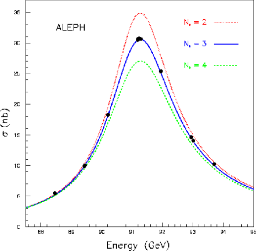
Figure 1: The line-shape of the Z-resonance in $e^{+}e^{-}$ scattering as a function of the center of mass energy [1, 2, 3, 4]. The theoretical prediction is shown under the assumption that nature contains $N_{\nu}$ different neutrinos (Figure taken from [1]).

The gauge theory for the strong force is called Quantum Chromodynamics (QCD), in which quarks and gluons assume the rôles of the electrons and photons of QED. Quarks are the constituents of the more familiar protons and neutrons. The coupling constant of QCD, $\alpha_{s}$, then characterizes the strength of the interaction between quarks and gluons in a similar manner as the fine structure constant does in QED. One important property of all coupling “constants” in the Standard Model is that they depend on the energy transfer $\mu$ in the interaction process. In this sense they are not really constant, and one usually refers to them as couplings that “run” with the energy scale. For instance, at $\mu\approx 100\,{\rm GeV}$ the strong coupling constant has been determined as $\alpha_{s}=0.12$. Although this is much larger than the fine structure constant of QED, the method of perturbation theory still works well. However, if the energy scale $\mu$ is decreased from $100\,{\rm GeV}$ it is found that the value of $\alpha_{s}$ increases. In fact, at $\mu\approx 1\,{\rm GeV}$ it becomes so large that perturbation theory cannot be relied upon any more. It is then obvious that particle theorists require a tool which is able to deal with large values of $\alpha_{s}$. In other words, what is needed is a non-perturbative method to work out the predictions of QCD in this situation.

As mentioned before, the simple and elegant theory of QCD is formulated in terms of quarks and gluons. Evidence for their existence has been accumulated in scattering experiments at high energies. Yet what is observed in experiments at low energies, say, $\mu\lesssim 1\,{\rm GeV}$ are protons, neutrons, $\pi$-mesons and many other particles, all known as hadrons. In fact, a striking property of QCD is “confinement”, which means that quarks and gluons cannot be produced in experiments. Intuitively this property of QCD can be understood in terms of the strong growth of forces between quarks as their separation increases. Thus, the only directly observable particles are the bound states of quarks and gluons, i.e. the hadrons.

Particle physicists are then faced with the task of connecting the theoretically rather simple regime of QCD at high energies with the properties of protons, $\pi$-mesons and other hadrons observed at low energies. This task is made all the more difficult since analytic methods such as perturbation theory fail completely to describe the world of hadrons. This has led to the development of numerical techniques, namely computer simulations of QCD formulated on a discrete lattice of space-time points. This method allows for a non-perturbative treatment of the theory in the low-energy regime.

The basic reason why the two regimes can be connected is the fact that QCD contains only the fundamental gauge coupling $\alpha_{s}$ and the masses of the quarks as free parameters. All observables, such as the mass of the proton, can in principle be predicted in terms of these quantities. The ALPHA Collaboration has embarked on a project to connect low and high energies in practice, by means of extensive computer simulations of lattice QCD. Following the original idea of [5], new methods have been developed and applied, which have yielded rather precise results. It is then possible to turn the tables: starting from the accurate experimental information on the properties of hadrons, the fundamental parameters of QCD can be determined numerically.

In particular, the high-energy behaviour of the strong coupling constant $\alpha_{s}$ is given by

$$\alpha_{s}^{-1}\,\stackrel{{\scriptstyle\mu\rightarrow\infty}}{{\propto}}\,\ln\left({\mu\over\Lambda}\right)\,,$$ (1)

This implies that the energy dependence of $\alpha_{s}$ is specified completely in terms of a single parameter, $\Lambda$, measured in energy units. It is only natural to take $\Lambda$ as a basic parameter of QCD instead of the energy-dependent $\alpha_{s}$. The ratio of $\Lambda$ to the proton mass is computable in lattice simulations – but not in perturbation theory. Thus, one of the main goals of the ALPHA Collaboration is the precise determination of $\Lambda$.

Figure 2: Two dimensional slice of a 4-dimensional space-time lattice. Red (yellow) points at the bottom (left) are identified with those at the top (right) by periodic boundary conditions.

With QCD being one of the pillars of the Standard Model, it is clear that the precise knowledge of its parameters such as $\Lambda$ is important for the ongoing quest for generalizations of the Standard Model. Such more complete theories are needed to describe the early stages of the universe and are also expected to be relevant at energies which will be accessible at future particle colliders.

2 Lattice QCD

In the mathematical formulation of QCD, the basic quantities are quark and gluon fields, which are functions of the space-time coordinates $x_{\mu}$, with $x_{0}$ identified with time. The classical field equations, which describe their dynamics, are differential equations – generalizations of Maxwell’s equations for electromagnetism. To allow for a numerical treatment, it is then natural to discretize the differential equations with a discretization length $\color[rgb]{1,0,1}a$, termed the lattice spacing. This procedure turns differential operators into finite difference operators and the fields are defined only at the points of a space-time lattice, illustrated in Fig. 2.

Quantization is achieved by Feynman’s path integral representation. It involves integrations over all degrees of freedom weighted with the exponential of the classical action. Let $\Omega$ denote an observable, represented e.g. by a combination of quark and antiquark fields. Its expectation value, $\langle\Omega\rangle$, is defined as ⟨Ω⟩= 1Z∫D[U]D [¯ψ,ψ] Ω  e^-S_G[U]-S_F[U,¯ψ,ψ], where $Z$ is fixed by the condition $\langle\mathchoice{\rm 1\kern-5.20004pt{1}}{\rm 1\kern-5.20004pt{1}}{\rm 1\kern-3.99994pt{1}}{\rm 1\kern-3.99994pt{1}}\rangle=1$. To further prepare for an evaluation of the path integral on a computer, the quark degrees of freedom are integrated out analytically. The expression for $\langle\Omega\rangle$ then becomes ⟨Ω⟩= 1Z∫D[U] Ω_eff {det(D[U])}^N_f  e^-S_G[U]. $\Omega_{\rm eff}$ denotes the representation of $\Omega$ in the effective theory, where only gluon fields remain in the path integral measure. Equation (2) requires some further explanation:

• $D[U]$ denotes the Dirac operator, and for simplicity of presentation we have considered QCD with $N_{\rm f}$ quarks of equal mass $m$, which enters $D[U]$. For hadron physics at small energies the case $N_{\rm f}=3$ is most relevant. The heavier quarks decouple from the dynamics up to small effects;

• The gluon field is represented by link variables $U(x,\mu)$ connecting the sites $x$ and $x+a\hat{\mu}$ (shown as in Fig. 2). The measure ${\cal D}[U]$ is the product of integration measures for each link;

• The action $S_{\rm G}[U]$ is a sum of local terms over the lattice, coupling only gluon variables within one plaquette ( in Fig. 2). By contrast, the effective interaction resulting from the integration over the anticommuting quark fields is of infinite range: although the finite difference Dirac-operator $D[U]$ is local, $\det(D[U])$ couples gluons at arbitrary distances.

• Using the representation eq. (2), our expression for $\langle\Omega\rangle$ has the form of a thermal average in statistical mechanics, and one may use stochastic sampling to evaluate the integral if the space-time volume is made finite by restricting $0\leq x_{\mu}<L$.

• As an example, consider $\langle\Phi(x)\Phi^{\dagger}(y)\rangle$ where $\Phi(x)$ is a suitable combination of quark fields at a point $x$, which has the quantum numbers of some hadron. The expectation value is then proportional to the quantum-mechanical amplitude for the propagation of the hadron from point $y$ to $x$, from which the mass of the hadronic bound state may be obtained.

The lattice formulation sketched above leads to a mathematically well-defined expression for $\langle\Omega\rangle$. In particular, the typical infinities which are encountered in field theoretical expectation values are absent.

The exact treatment of the determinant, eq. (2), still presents a major challenge, even on today’s massively parallel computers. In many applications one has therefore set $N_{\rm f}=0$. This – very drastic – approximation defines the so-called quenched approximation. Physically it means that the quantum fluctuations of quarks are neglected and only those due to the gluons are taken (exactly) into account. Although it turns out that the quenched approximation works well at the 10%-level, the proper treatment for $N_{\rm f}>0$ is perhaps the most important issue in current simulations.

Whether or not the quenched approximation is employed, one always has to address the problem of lattice artefacts. Let $R$ denote a dimensionless observable, such as a ratio of hadron masses. Then its expectation value on the lattice differs from the value in the continuum by corrections of order $a^{p}$:

$$R^{\rm lat}=R^{\rm cont}+O(a^{p}),$$ (2)

where the power $p$ depends on the chosen discretization of the QCD action. The correction term for typical values of $a$ can be quite large, and an extrapolation to the continuum limit is then required to obtain the desired result. If $p$ is large, the rate of convergence to the continuum limit is high, and hence the extrapolation is much better controlled.

Let us now return to the problem of determining the energy dependence of quantities such as the running coupling $\alpha_{s}$. Obviously the numerical simulation is possible only if the number of points of the lattice, $(L/a)^{4}$, is not too large; typical lattice sizes are $L/a\leq 32$. Therefore, besides $a$ also the effect of the finite value of $L$ has to be considered. It is known rather well that $L=2\,{\rm fm}$ is sufficient for most quantities, and that much smaller volumes would lead to unacceptably large corrections to the desired $L\to\infty$ limit. A physical box size of $L=2\,{\rm fm}$ together with $L/a\leq 32$ thus implies a $\stackrel{{\scriptstyle\textstyle{>}}}{{\sim}}$ 0.05 fm. The existence of such a lower bound on $a$, imposed by practicability considerations, also means that the energies, $\mu$, that can be expected to be treated correctly have to satisfy μ≪a^-1 ≲4 GeV . In other words, lattice QCD is well suited for the computation of low energy properties of hadrons, while high energies appear impossible to reach. The ALPHA Collaboration has developed and applied an approach to circumvent this problem, which is described below.

3 Running coupling and quark masses

We are now going to outline the strategy which allows to connect the low- and high-energy regimes of QCD in a controlled manner. Results for the $\Lambda$ parameter and the quark masses will then be presented. From now on we will drop the subscript “s” on the strong coupling constant $\alpha_{s}$.

3.1 Gedankenexperiment

From the above it is evident that the restriction of numerical lattice QCD to low energies is necessary to avoid finite-size effects (FSE) when working with a manageable number of lattice sites. For the computation of an effective coupling, this problem can be circumvented since one has great freedom in the definition of such a coupling. Even the strength of finite-size effects serve as a measure of the interactions of the theory, and thus a suitably chosen FSE may be used to define [5] an

$$\color[rgb]{1,0,0}\text{effective coupling }\;\bar{g}(L)\color[rgb]{0,0,0}\;\text{with}\;\alpha(\mu)={\bar{g}^{2}(L)\over 4\pi}\,,\;\color[rgb]{1,0,0}\mu=1/L\,\color[rgb]{0,0,0}.$$ (3)

It depends on (“runs with”) the energy scale $\mu=1/L$. Such a coupling can be computed in the regime $\mu\ll a^{-1}$ requiring only a moderate resolution of the space-time world; $L/a={\rm O}(10)$ points per coordinate are sufficient.

In a numerical calculation, the success of this general idea will depend on a few properties of the coupling. It must be computable with good statistical precision in a Monte Carlo (MC) simulation, and with small discretization errors. Furthermore, one would like to know its scale dependence analytically for large energies. This is achieved by determining the perturbative expansion of the so-called $\beta$-function,

$$\beta(\bar{g})=-L{\partial\bar{g}\over\partial L} \buildrel{\bar{g}}\rightarrow 0\over{\sim}\, -{\bar{g}}^{3}\left\{b_{0}+b_{1}{\bar{g}}^{2}+b_{2}{\bar{g}}^{4}+\ldots\right\},$$ (4)

to the order indicated above, or even higher.

Figure 3: The boundary conditions used for the definition of the finite-size coupling $\bar{g}(L)$ in QCD.

In QCD, a coupling with these properties could indeed be found [6, 7, 8]. Its definition starts from QCD in a box of size $L^{4}$. Periodic boundary conditions are imposed for the fields as functions of the three spatial coordinates, and Dirichlet boundary conditions are set in the time-direction, as shown in Fig. 3. The Dirichlet boundary conditions are homogeneous except for the spatial components of the gluon gauge potentials, $A_{k}$. With this choice of boundary conditions the topology is that of a 4-dimensional cylinder.

Classically, these boundary conditions lead to a homogeneous (${\it\bf x}$ and $t$ independent) colour-electric field inside the cylinder. The walls at time $t=0$ and $t=T$ act quite similarly to the plates of an electric condensor. The strength of the QCD interactions is conveniently defined in terms of the colour-electric field at the condensor plates: ¯g^2(L) = E_classical ⟨E ⟩  . Here $E$ is a special colour component of the electric field.

For weak coupling, i.e. for small $L$, the path integral is dominated by field configurations which correspond to small fluctuations about the classical solution. On the other hand, for $L\approx 1\,{\rm fm}$ they may deviate significantly from the classical solution, and this can be realized in a MC-simulation of the path integral.

3.2 The running coupling

The energy dependence of the coupling $\bar{g}^{2}(L)$ can be determined recursively through a number of compute-effective steps. Figure 4 illustrates the implementation of the recursion

$$\bar{g}^{2}(2L)=\sigma(\bar{g}^{2}(L))\,.$$ (5)

Figure 4: The recursion to compute $\bar{g}(L)$ with $L=L_{0}\color[rgb]{1,0,1}\to\color[rgb]{0,0,0}2L_{0}\color[rgb]{1,0,1}\to\color[rgb]{0,0,0}4L_{0}\color[rgb]{1,0,1}\to\color[rgb]{0,0,0}8L_{0}$. It is iterated further until one arrives at $2^{n}L_{0}$, in practice $n\sim 8$. One always alternates between keeping $a$ fixed and increasing $L\to 2L$ and keeping $L$ fixed and increasing $a$.

The function $\sigma$ describes the change in the coupling when the physical box size is doubled. Since the relevant energy scale for the running of the coupling ($\mu=1/L$) is separated from the lattice spacing $a$, one may compute $\sigma$ recursively over several orders of magnitude in $\mu$, whilst keeping the number of lattice sites at a manageable level, i.e. $L/a={\rm O}(10)$.

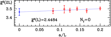
Figure 5: The extrapolation of the function $\bar{g}^{2}(2L)=\sigma(\bar{g}^{2}(L))$ from the data at finite lattice spacing $a$ to the continuum (blue square).

The results of one horizontal step in Fig. 4, performed on the APE-computers at NIC/Zeuthen, is displayed in Fig. 5. They are shown as a function of the resolution $a/L$. Because the coupling and the details of the discretization were chosen with great care, the dependence on the resolution is tiny and the lattice numbers can be extrapolated to the continuum $a/L\to 0$. To arrive at the continuum limit, each of the horizontal steps in the figure is indeed repeated several times with different resolutions!

In this way, the continuum function $\sigma(u)$ was obtained for a range of $u=\bar{g}^{2}(L)$. Starting from a minimal value of $u$, the recursive application of eq. (5) yields the points in Fig. 6. They may be compared to the integration of the differential equation (4) towards low values of $\mu$, starting at the lowest value of $\alpha$. One then makes the important observation, that eq. (4), truncated at the indicated order, is quantitatively verified in the region of low enough $\alpha$. It may hence also be used to compute the $\Lambda$-parameter from ($\bar{g}=\bar{g}(L=1/\mu)$)

$$\Lambda = \mu\,(b_{0}\bar{g}^{2})^{-b_{1}/2b_{0}^{2}}{\rm e}^{-1/2b_{0}\bar{g}^{2}}\times\exp\left\{-\int_{0}^{\bar{g}}{\rm d}g\left[{1\over\beta(g)}+{1\over b_{0}g^{3}}-{b_{1}\over b_{0}^{2}g}\right]\right\},$$ (6)

with negligible errors due to higher-order terms that are not included.

The attentive reader will have noticed that the computation explained so far, “only” determines the dependence of $\alpha$ on the combination $\mu/\Lambda$, while in the figure we show it as a function of $\mu$ in physical units for $N_{\rm f}=0$, i.e. in the quenched approximation. The missing link is to connect the lowest energy $\mu=1/L_{\rm max}$ contained in the figure, to a low energy – experimentally accessible – property of a hadron. The connection with the decay rate of the K-meson [9], which we do not describe here, yields the physical units shown in the figure as well as the final result

$$\Lambda=238(19)\,{\rm MeV}\text{ for }N_{\rm f}=0\,.$$ (7)

Currently, the ALPHA Collaboration is extending these computations to the numerically very demanding case of $N_{\rm f}=2$. First promising results, which are still awaiting a final check for the absence of discretization errors are shown on the r.h.s. of Fig. 6. The step to connect $L_{\rm max}$ to a low-energy observable has yet to be performed, and hence the results are plotted as a function of $\mu/\Lambda$. It is worth pointing out that, in order to ensure efficiency and correctness of these $N_{\rm f}>0$ simulations, the development and testing of MC-algorithms is very important [10, 11, 12].

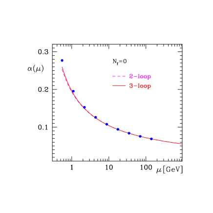
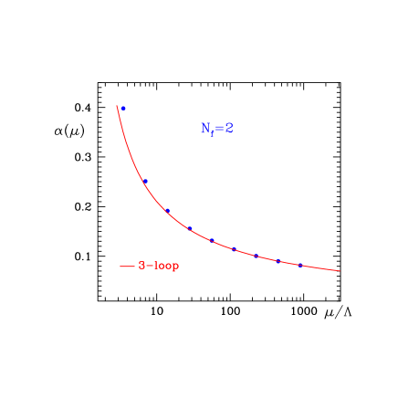
Figure 6: The energy dependence of the coupling as computed from lattice QCD (points) compared to the perturbative expression eq. (4) with the $b_{2}$-term (full line) and without.

3.3 Quark masses

The masses of the quarks are of a very different nature from the mass of the electron. The fundamental difference is the property of confinement mentioned in section 1. It means that a quark can not be prepared in isolation to perform an experimental measurement of its mass. Consequently, quark masses have to be understood as parameters of the theory, and their proper definition very much resembles that of an effective coupling. In particular, they have an energy dependence similar to the one of $\alpha$. When defined in a natural way [13], the energy dependence is the same for all quark flavours; in other words, ratios of quark masses do not depend on the energy. The overall energy dependence has been determined with the same strategy as the one described for $\alpha$ and in fact with similar precision (see Fig. 2 in [13]).

The numerical values of the quark masses (at a particular low energy scale) are conveniently extracted by relating them to the masses of quark-antiquark bound states with pseudoscalar quantum numbers: $\pi$-, K-, D-, B-mesons. Results of the ALPHA Collaboration obtained in the $N_{\rm f}=0$ approximation are shown in Fig. 7 in two different (common) conventions.  The upper row shows the running masses $\kern 1.0pt\overline{\kern-1.0ptm\kern-1.0pt}\kern 1.0pt$ in the so-called ${\rm\overline{MS\kern-0.50003pt}\kern 0.50003pt}$ scheme at a renormalization energy $\mu=2\,{\rm GeV}$, while the lower one shows the so-called renormalization group invariant quark masses. The latter are related to the running quark masses via

$$M=\lim_{\mu\to\infty}\kern 1.0pt\overline{\kern-1.0ptm\kern-1.0pt}\kern 1.0pt(\mu)\left[2b_{0}\left(\bar{g}(\mu)\right)^{2}\right]^{-d_{0}/2b_{0}}\,,$$ (8)

where $d_{0}$ characterizes the asymptotic behavior of $\kern 1.0pt\overline{\kern-1.0ptm\kern-1.0pt}\kern 1.0pt(\mu)$ for large energy. It is computable in perturbation theory and has a value of $d_{0}=8/(4\pi)^{2}$.

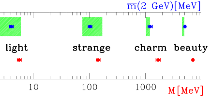
Figure 7: Quark masses determined by the ALPHA collaboration in the $N_{\rm f}=0$ approximation [16, 13, 9, 17, 15]. The label “light” denotes the average mass of the up and the down quark mass. Green shaded areas show the error band quoted by the particle data group [18].

4 Improvement

Equation (2) shows that lattice and continuum quantities differ by discretization errors. In Wilson’s formulation of lattice QCD these discretization effects are of order $a$, which can be quite large. People have therefore tried to find an improved version of the Wilson action, so that the deviation of observables computed on the lattice to their continuum values is of O($a^{2}$), or even higher.

In order to illustrate the problem, let us consider the solution of differential equations by means of numerical integration. Given the initial value problem

$${{{\rm d}y}\over{{\rm d}x}}=f(x,y),\quad y(x_{0})=y_{0},$$ (9)

the well-known Euler method provides a formula for its numerical solution, i.e.

$$y_{j+1}=y_{j}+a\,f(x_{j},y_{j}),\quad j=0,1,2,\ldots.$$ (10)

Here the quantity $a$ denotes the finite step size used to approximate the derivative ${{\rm d}y}/{{\rm d}x}$ in terms of finite differences. In order to compute the solution at point $x=x_{0}+na$ for a fixed value of $a$ one has to perform $n$ iteration steps. The central question then is by how much this solution deviates from the exact one. For the simple Euler method one can show that this so-called truncation error is proportional to $a^{2}$. Obviously the accuracy of the solution will be larger for small $a$, but then the number of iterations, $n$, may become very large. It is much more efficient to use an improved solution scheme, such as the Runge-Kutta method. Here the function $f$ in eq. (10) is replaced by a more complicated expression, which is chosen in such a way that the truncation error is proportional to $a^{5}$.

The analogy of this example with lattice QCD is obvious: the step size is now the lattice spacing, and the lattice action must be chosen such that the leading discretization error is of higher order in $a$. However, in a quantum field theory like QCD the search for an improved action is not straightforward: although one can quite easily write down an action which formally has O($a^{2}$) artefacts, the interactions between quarks and gluons in the discretized theory can again introduce O($a$) errors at the quantum level.

To be more explicit, let $S_{\rm W}$ denote the Wilson action for lattice QCD. Sheikholeslami and Wohlert [19] have shown that it is sufficient to add just one more interaction term, corresponding to an action $\delta{S}$, to $S_{\rm W}$ in order to cancel its leading discretization error proportional to $a$. To ensure that quantum effects do not introduce O($a$) effects “via the back door”, the term $\delta{S}$ has to be multiplied by a coefficient $c_{\rm sw}$. This improvement coefficient must be suitably tuned in order to achieve the complete cancellation of O($a$) artefacts at the quantum level for observables such as hadron masses. The O($a$) improved version of Wilson’s action then reads

$$S_{\rm SW}=S_{\rm W}+c_{\rm sw}\delta{S}.$$ (11)

The ALPHA Collaboration has developed and applied a method to determine $c_{\rm sw}$ in computer simulations [20, 21, 22, 23]. The method amounts to computing the expectation value of a pure lattice artefact as a function of $c_{\rm sw}$. The value of $c_{\rm sw}$ at the point where the artefact vanishes then defines the improved action for the corresponding value of the lattice spacing. Thus, non-perturbative methods are not only used to compute physical observables, but also to improve the reliability of the numerical treatment of the theory as such. The improved action is only slightly more complicated to implement in practical simulations. The increased effort is easily offset by the faster convergence to the continuum limit. As a result, the action with $c_{\rm sw}$ as determined in [22, 23] has by now become a standard for precision lattice QCD computations. In particular this improvement was essential in obtaining most of the results quoted in the previous section.

Of course, one also has to verify that observables computed with the improved action indeed approach the continuum limit with a rate proportional to $a^{2}$. Tests of this kind have been performed successfully (see, e.g. ref. [24]), and other examples for the effectiveness of the improvement programme for the evaluation of many hadronic observables can be found in [9].

5 Machines and resources

Although conceptual advances like O($a$) improvement are of great importance, progress in lattice QCD is also dependent on the availability of sufficient computer resources.

In the 1980s most simulations were performed on vector supercomputers like the Cray X-MP. Since then the demand for increased performance has led to the development of massively parallel machines, which are now widely used. Lattice QCD is a problem which lends itself easily to parallelization: the total volume can be divided into many sublattices, which are distributed over a grid of processors. The latter can perform the same task on independent data. Furthermore, the communication pattern for lattice QCD is simple, since most algorithms only require nearest-neighbour communications.

The ALPHA Collaboration has mostly used parallel computers from the APE family of machines [25, 26, 27, 28]. The latest generation, APEmille, has been developed jointly by INFN and DESY. The smallest entity in the APEmille processor grid consists of a cube of $2\times 2\times 2$ processors. These cubes are then connected to form larger grids. Despite its very conservative clock speed of 66 MHz, each processor achieves a peak performance of 528 MFlops, thanks to the optimization for complex arithmetic: the operation $a\times{b}+c$, which requires 8 floating point operations for the three 32-bit complex numbers $a,\,b$ and $c$, is performed in one clock cycle. The total peak speed of the current installation of APEmille machines at DESY-Zeuthen amounts to more than 500 GFlops (single precision).

The programming language for APEmille is TAO, which has a FORTRAN-like syntax, but also includes special features designed to facilitate parallelization and coding, and allows to achieve a high proportion of the peak speed. One such feature is the easy access to any desired number of the 512(!) registers. The typical efficiency of ALPHA-programs on APEmille is about 30% of the peak speed. A similar figure has been achieved by other lattice QCD collaborations on machines like the Cray T3E, but at the price of having to code the core routines in assembler language [29]. An interesting figure-of-merit is the price/performance ratio. For APEmille it is $(8-10)$ Euro per sustained MFlops and there are efforts under way to reduce this number much further. In addition it was also demonstrated that PC clusters with Myrinet network can achieve about $3-4$ Euro/MFlops sustained [30]. These developments let us await the future with optimism.

6 Future

Moving towards the realistic case of $N_{\rm f}=3$ should soon be possible. Once this has been achieved, the most precise determinations of the fundamental parameters of QCD may come from the low energy hadron spectrum combined with lattice QCD to evaluate the theory. The methods developed in this project are expected to play an important rôle in this program.

Furthermore these methods and related ones [31, 32, 33] will improve the reliability of the determination of properly normalized weak decay (and mixing) amplitudes of hadrons [34]. Their knowledge is again of vital importance in tests of the Standard model and the search for an even more fundamental theory.

The results presented in this article were obtained on the APE100 and APEmille installations at Zeuthen. The total CPU time required was about $10^{7}$ processor-hours on APE100 and $0.2\cdot 10^{7}$ processor-hours on APEmille, respectively.

References

- [1] See: http://alephwww.cern.ch/ALEPHGENERAL/reports/figures/ew/index.html
- [2] ALEPH, DELPI, L3 and OPAL Collaborations. Combination procedure for the precise determination of z boson parameters from results of the LEP experiments. hep-ex/0101027, 2001.
- [3] R. Barate et al. Measurement of the Z-resonance parameters at LEP. Eur. Phys. J., C14:1–50, 2000.
- [4] G. Abbiendi et al. Precise determination of the Z-resonance parameters at LEP: ’Zedometry’. Eur. Phys. J., C19:587–651, 2001.
- [5] Martin Lüscher, Peter Weisz and Ulli Wolff. A numerical method to compute the running coupling in asymptotically free theories. Nucl. Phys., B359:221–243, 1991.
- [6] Martin Lüscher, Rainer Sommer, Ulli Wolff and Peter Weisz. Computation of the running coupling in the SU(2) Yang-Mills theory. Nucl. Phys., B389:247–264, 1993.
- [7] Martin Lüscher, Rainer Sommer, Peter Weisz and Ulli Wolff. A precise determination of the running coupling in the SU(3) Yang-Mills theory. Nucl. Phys., B413:481–502, 1994.
- [8] Stefan Sint and Rainer Sommer. The running coupling from the QCD Schrödinger functional: A one loop analysis. Nucl. Phys., B465:71–98, 1996.
- [9] Joyce Garden, Jochen Heitger, Rainer Sommer and Hartmut Wittig. Precision computation of the strange quark’s mass in quenched QCD. Nucl. Phys., B571:237–256, 2000.
- [10] Roberto Frezzotti, Martin Hasenbusch, Ulli Wolff, Jochen Heitger and Karl Jansen. Comparative benchmarks of full QCD algorithms. Comput. Phys. Commun., 136:1–13, 2001.
- [11] M. Hasenbusch. Speeding up finite step-size updating of full QCD on the lattice. Phys. Rev., D59:054505, 1999.
- [12] Martin Hasenbusch. Speeding up the Hybrid Monte Carlo algorithm for dynamical fermions. Phys. Lett., B519:177–182, 2001.
- [13] Stefano Capitani, Martin Lüscher, Rainer Sommer and Hartmut Wittig. Non-perturbative quark mass renormalization in quenched lattice QCD. Nucl. Phys., B544:669, 1999.
- [14] H. Leutwyler. The ratios of the light quark masses. Phys. Lett., B378:313–318, 1996.
- [15] Jochen Heitger and Rainer Sommer. A strategy to compute the b-quark mass with non-perturbative accuracy. Nucl. Phys. Proc. Suppl., 106:358–360, 2002.
- [16] Stefan Sint and Peter Weisz. The running quark mass in the SF scheme and its two loop anomalous dimension. Nucl. Phys., B545:529, 1999.
- [17] Juri Rolf and Stefan Sint. The charm quark’s mass in quenched QCD. Nucl. Phys. Proc. Suppl., 106:239–241, 2002.
- [18] D. E. Groom et al. Review of particle physics. Eur. Phys. J., C15:1–878, 2000.
- [19] B. Sheikholeslami and R. Wohlert. Improved continuum limit lattice action for QCD with Wilson fermions. Nucl. Phys., B259:572, 1985.
- [20] Martin Lüscher, Stefan Sint, Rainer Sommer and Peter Weisz. Chiral symmetry and O() improvement in lattice QCD. Nucl. Phys., B478:365–400, 1996.
- [21] M. Lüscher and P. Weisz. O() improvement of the axial current in lattice QCD to one-loop order of perturbation theory. Nucl. Phys., B479:429–260, 1996.
- [22] Martin Lüscher, Stefan Sint, Rainer Sommer, Peter Weisz and Ulli Wolff. Non-perturbative O() improvement of lattice QCD. Nucl. Phys., B491:323–343, 1997.
- [23] Karl Jansen and Rainer Sommer. O() improvement of lattice QCD with two flavors of Wilson quarks. Nucl. Phys., B530:185–203, 1998.
- [24] Jochen Heitger. Scaling investigation of renormalized correlation functions in O() improved quenched lattice QCD. Nucl. Phys., B557:309–326, 1999.
- [25] A. Bartoloni et al. A hardware implementation of the APE100 architecture. Int. J. Mod. Phys., C4:995, 1993.
- [26] A. Bartoloni et al. The software of the APE100 processor. Int. J. Mod. Phys., C4:969, 1993.
- [27] P. Vicini et al. The teraflop supercomputer APEmille: Architecture, software and project status report. Comput. Phys. Commun., 110:216–219, 1998.
- [28] A. Bartoloni et al. Status of APEmille. Nucl. Phys. Proc. Suppl., 106:1043–1045, 2002.
- [29] C.R. Allton et al. Light hadron spectroscopy with O() improved dynamical fermions. Phys. Rev. D60:034507, 1999; Stephen Pickles, private communication.
- [30] Martin Lüscher. Lattice QCD on PCs? Nucl. Phys. Proc. Suppl., 106:21–28, 2002.
- [31] Roberto Frezzotti, Pietro Antonio Grassi, Stefan Sint and Peter Weisz. Lattice QCD with a chirally twisted mass term. JHEP, 08:058, 2001.
- [32] Roberto Frezzotti, Stefan Sint and Peter Weisz. O() improved twisted mass lattice QCD. JHEP, 07:048, 2001.
- [33] M. Guagnelli, J. Heitger, C. Pena, S. Sint and A. Vladikas. mixing from the Schrödinger functional and twisted mass QCD. Nucl. Phys. Proc. Suppl., 106:320–322, 2002.
- [34] G. Martinelli. Matrix elements of light quarks. Nucl. Phys. Proc. Suppl., 106:98–110, 2002.