Parallel J-W Monte Carlo Simulations of Thermal Phase Changes in Finite-size Systems

Abstract

The thermodynamic properties of $(TeF_{6})_{59}$ clusters that undergo temperature-driven phase transitions have been calculated with a canonical J-walking Monte Carlo technique. A parallel code for simulations has been developed and optimized on SUN3500 and CRAY-T3E computers. The Lindemann criterion shows that the clusters transform from liquid to solid and then from one solid structure to another in the temperature region 60-130 K.

1 Introduction

The interest in phase transitions in finite systems is two-fold: firstly, bulk properties of the material can be simulated if the system is studied under periodic boundary conditions [1] and proper account for rounding and shifting of the measurable quantities is taken in the analysis. Secondly, free finite systems, such as molecular clusters, are of interest due to their peculiar properties, which are not observed in bulk systems of the same substance [2]. These are important for the synthesis of nanomaterials and nanodevices [3].

We use a canonical Monte Carlo (MC) method to investigate temperature-induced critical behavior in clusters containing 59 $TeF_{6}$ molecules.

Our model system contains 59 octahedral rigid $TeF_{6}$ molecules which are allowed to rotate and translate. Their interaction is reliably described by a Lennard-Jones and a Coulomb atom-atom potential:

$$V({\bf q}) = \sum\limits_{i<j}{}U(r_{ij})$$ (1)

$$V({\bf q}) = \sum\limits_{i<j}{}\sum\limits_{\alpha,\beta}4\epsilon_{\alpha\beta}\left[\left(\frac{\sigma_{\alpha\beta}}{r_{ij}}\right)^{12}-\left(\frac{\sigma_{\alpha\beta}}{r_{ij}}\right)^{6}\right]+$$

$$+ \sum\limits_{i<j}{}\sum\limits_{\alpha,\beta}\left(\frac{q_{i\alpha}q_{i\beta}}{r_{ij}}\right)$$

where ${\bf q}$ is a generalized coordinate; $r_{ij}$ is the distance between the $i-th$ and $j-th$ atom. The indices $\alpha,\beta$ denote either a fluorine or a tellurium atom. The parameter values are taken from [4].

This orientation-dependent potential generates rugged potential energy surfaces. How to tackle the behavior of a system having a rugged potential energy surface in MD simulations is discussed in [5, 6].

Here we tackle the problem with the help of the jump-walking Monte Carlo method, [7, 8], which is a smart development of the Metropolis algorithm. We have parallelized the code to speed up the computations [9].

2 J-walking algorithm

In its general form, the method generates trial moves from a higher-temperature $(T_{J})$ equilibrium distribution with a probability specified by the variable $P_{J}$:

$$P=min{}\left\{1,q[x^{*}|x]\right\}$$ (2)

where the Metropolis probability function is:

$$q(x^{*}|x)=e^{-(\frac{1}{T}-\frac{1}{T_{J}})\left\{V(x^{*})-V(x)\right\}}$$ (3)

$V(x)$ is the potential energy of the system at a temperature $T$ and $V(x^{*})$ is the potential energy of a new configuration at the temperature $T_{J}$.

The remaining trial moves are of conventional Metropolis character.

In our study we use multi-temperature generalizations [10] of the basic approach.

We develop a parallel J-walking code that enables us to carry out a Monte Carlo simulation efficiently in a multiprocessor computing environment. We apply the code in the study of the thermodynamic properties of $(TeF_{6})_{n}$, $n=59$ clusters.

The J-walking technique can be implemented in two ways. The first approach is to write the configurations from the simulation at the J-walking temperature to an external file and access these configurations randomly, while carrying out a simulation at the lower temperature. It is necessary to access the external files randomly to avoid correlation errors [11]. The large storage requirements limit the application of the method to small systems. The second approach uses tandem walkers, one at a high temperature where Metropolis sampling is ergodic and multiple walkers at lower temperatures.

The best features of these two approaches can be combined into a single J-walking algorithm [12] with the use of multiple processors and the Message Passing Interface (MPI) library. We incorporate MPI functions into the MC code to send and receive configuration geometries and potential energies of the clusters. Instead of generating external distributions and storing them before the actual simulation, we generate the required distributions during simulation and pass them to the lower-temperature walkers.

Parallel J-walking algorithm:

• Step 1. For each t make Metropolis MC steps:

  • Rotate each molecule.

  • Translate each molecule.

  • Reject or accept step.

  • Go to step 1.

• Step 2. After $S_{1}$ steps - collect statistics:

  • Potential energy histogram.

  • Energy average and deviation.

  • Heat capacity $C_{V}$.

  • Save current configuration.

• Step 3. After $S_{2}$ steps - make jump-walking step by exchanging the configurations using MPI.

• Step 4. Go to step 1.

The diagram of model J-walking is shown in fig.1. Each square is a Metropolis MC simulation at a particular temperature. The set of boxes on the right-hand side represents the array of previous configurations of the system, which are stored in the memory to avoid correlations between the lower and the higher temperature. At each trial jump we randomly choose one of the 4 systems. When a configuration is transmitted to a lower-temperature process, it is a configuration randomly chosen from the array of higher-temperature walkers. The current configuration of the walker then replaces the configuration just passed from the array to another temperature. In fig.2 we show the parallel decomposition of computation. Each process computes part of one of 4 multistage J-walking chains, and exchanges configurations and energy with others.

We use array sizes of 2500 configurations. The number of configurations is limited by the processor RAM used in simulation. In the parallelization implemented in our code, the arrays are small and do not inhibit applications of the method to large systems. For the computations in the present work the number of MC passes for each temperature is $6.10^{5}$ for each cluster containing 59 $TeF_{6}$ molecules (413 atoms). We make J-walk jump attempts at every 50 Metropolis MC steps during the thermalisation and at every 150 steps during the main computation.

The computer code has been ported, tested and optimized on SUN 3500 and CRAY-T3E machines. In our program dynamic memory management has been implemented for optimal usage of the memory. We find that memory and performance requirement make CRAY-T3E more suitable for such computations. In our runs we use 64 processors each with 64 MB RAM. Each run of $6.10^{5}$ steps takes approximately 11h per CPU.

3 Results and Conclusions

Using the parallel code described in the previous section we make sets of production runs for 59 molecule clusters. The previous MD analysis of the temperature behavior of $TeF_{6}$ clusters pointed out a two-step structural transformation process [13] from an orientationally disordered bcc structure below cluster solidification to an orientationally oriented ordered monoclinic structure detected at low $T$ (below $20K$). The first step involves lattice reconstruction (bcc to monoclinic) and a partial order of one of the molecular axes, when the cluster is cooled down to its freezing point. This transition has been proved to be a first-order phase change [14] by detecting coexisting phases. A further temperature decrease causes complete orientational order of the three molecular axes. This transformation is continuous. The diagnostic method developed in [13] has been implemented to animate the solid-solid transformations [15].

To distinguish between the different phases, which the clusters adopt at different temperatures, we have computed the Lindemann index [16]:

$$\delta_{lin}=\frac{2}{N(N-1)}\sum\limits_{i,j(>i)=1}^{N}{\frac{\sqrt{<r_{ij}^{2}>-<r_{ij}>^{2}}}{<r_{ij}>}}$$ (4)

where $r_{ij}$ is the distance between the centers of the molecules ($Te$ atoms). For the values of $\delta_{lin}>0.08$ the system is in liquid phase and for $\delta_{lin}<0.08$ is in the solid phase. Fig.3 presents the Lindemann criterion for the 4 systems. The solidification occurs in interval $100K-115K$. In the interval $75K-80K$ the angle of the curve has changed.

We calculate the radial distribution function to reconstruct the crystal lattice. Fig.4 and fig.5 show the normalized radial distribution function for distances between centers of the $TeF_{6}$ molecules ($Te$ atoms). Fig.4 is at $157$. The peaks of the curve correspond to disordered liquid structure. Fig.5 is at $76K$ where the peaks correspond to an ordered structure (bcc lattice).

In this study a J-walking Monte Carlo algorithm has been implemented to study $(TeF_{6})$ clusters. A parallel J-walking code has been developed. Thermodynamic properties have been observed in the range from $60K$ to $150K$. We can compare the results to the results obtained from MD simulations.

Acknowledgments

The work was supported under the EC (contract No. HPRI-CT-1999-00026) TRACS-EPCC.

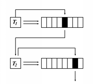
Figure 1: Diagram of a simple J-walking process. $T_{1}$ and $T_{2}$ present the systems at two different temperatures

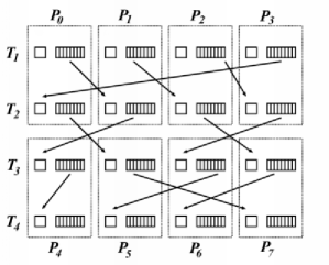
Figure 2: Diagram of a parallel decomposition of data and calculation between processors in J-walking algorithm. In this example we have 3 different systems at temperatures $T_{1}$, $T_{2}$, $T_{3}$ and $T_{4}$ distributed between 6 processors

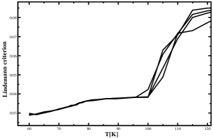
Figure 3: Lindemann criterion calculated for 4 clusters of 59 molecules.

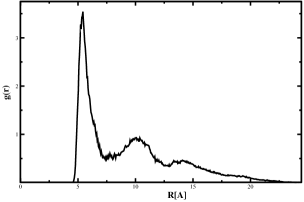
Figure 4: Radial distribution function for 59 molecule $TeF_{6}$ cluster at $157K$.

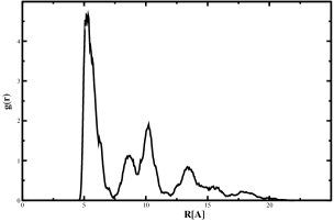
Figure 5: Radial distribution function for 59 molecule $TeF_{6}$ cluster at $76K$.

References

- [1] Monte Carlo Methods in statistical physics, edited by K. Binder (Springer - Berlin 1979).
- [2] A. Proykova and R. S. Berry, Z. Phys D. 40, (1997) 215.
- [3] A. Proykova, Physics (ISBN 0204 - 6946) 5, 2 (1999).
- [4] Kurtis E. Kinney, Shimin Xu, and Lawrence S. Bartell, J. Phys. Chem. 100, (1996) 6935.
- [5] A.Proykova, S. Pisov, R. S. Berry (to appear in JCP:AIPID 515140JCP).
- [6] A. Proykova, Bussei Kynkynu(Kyoto)76 (2001)62.
- [7] D.D. Frantz, D.L. Freeman, J.D. Doll, J. Chem. Phys. 93, (1990) 2769.
- [8] D.D. Frantz, D.L. Freeman, J.D. Doll, J. Chem. Phys. 97, (1992) 5713.
- [9] R.A. Radev, Parallel Monte Carlo simulation of critical behavior of finite systems, Report from the TRACS program, Edinburgh-UK (May-June 2000)
- [10] D.L. Freeman, J.D. Doll, Ann. Rev. Phys. Chem. 47, (1996) 43.
- [11] D.D. Frantz, J. Phys. Chem. 102, (1995) 3747.
- [12] A. Metro, D.L. Freeman, and Q. Topper, J. Chem. Phys. 104 (1996) 8690.
- [13] R. Radev, A. Proykova, Feng-Yin Li, R.S. Berry, J Chem. Phys. 109 (1998) 3596.
- [14] A. Proykova, I. Daykov and R.S.Berry, in Proc. of the Int.Thermo Symposium, (Bled, 11-14 June, 2000)
- [15] R.Radev, A. Proykova, R.S.Berry, http://www.ijc.com/articles/1998v1/36
- [16] F.A. Lindemann, Phys. Z. 11(1910) 609.