Manuscript Title:
Recurrence Plot Based Measures of Complexity and its Application to Heart Rate Variability Data

Abstract

The knowledge of transitions between regular, laminar or chaotic behavior is essential to understand the underlying mechanisms behind complex systems. While several linear approaches are often insufficient to describe such processes, there are several nonlinear methods which however require rather long time observations. To overcome these difficulties, we propose measures of complexity based on vertical structures in recurrence plots and apply them to the logistic map as well as to heart rate variability data. For the logistic map these measures enable us not only to detect transitions between chaotic and periodic states, but also to identify laminar states, i. e. chaos-chaos transitions. The traditional recurrence quantification analysis fails to detect the latter transitions. Applying our new measures to the heart rate variability data, we are able to detect and quantify the laminar phases before a life-threatening cardiac arrhythmia occurs thereby facilitating a prediction of such an event. Our findings could be of importance for the therapy of malignant cardiac arrhythmias.

I Introduction

Numerous scientific disciplines, such as astrophysics, biology or geosciences, use data analysis techniques to get an insight into the complex processes observed in nature Glass (2001); Blasius et al. (1999); Marvel (2001) which show generally a nonstationary and complex behavior. As these complex systems are characterized by different transitions between regular, laminar and chaotic behaviors, the knowledge of these transitions is necessary for understanding the process. However, observational data of these systems are typically rather short. Linear approaches of time series analysis are often not sufficient Goldberger et al. (1988); Glass and Kaplan (1993) and most of the nonlinear techniques (cf. Abarbanel et al. (1993); Kantz and Schreiber (1997)), such as fractal dimensions or Lyapunov exponents Kantz and Schreiber (1997); Kurths and Herzel (1987); Mandelbrot (1982); Wolf et al. (1985), suffer from the curse of dimensionality and require rather long data series. The uncritical application of these methods, especially to natural data, can therefore be very dangerous and it often leads to serious pitfalls.

To overcome these difficulties other measures of complexity have been proposed, such as the Renyi entropies, the effective measure complexity, the $\varepsilon$-complexity or the renormalized entropy Wackerbauer et al. (1994); Rapp et al. (2001). They are mostly based on symbolic dynamics and are efficient quantities for characterizing measurements of natural systems, such as in cardiology Kurths et al. (1995); Voss et al. (1996); Wessel et al. (2000a), cognitive psychology Engbert et al. (1997) or astrophysics Hempelmann and Kurths (1990); Schwarz et al. (1993); Witt et al. (1994). In this paper we focus on another type of measures of complexity, which is based on the method of recurrence plots (RP). This approach has been introduced for the analysis of nonstationary and rather short data series Casdagli (1997); Eckmann et al. (1987); Koebbe and Mayer-Kress (1992). Moreover, a quantitative analysis of recurrence plots has been proposed to detect typical transitions (e. g. bifurcation points) occurring in complex systems Trulla et al. (1996); Webber Jr. and Zbilut (1994); Zbilut and Webber Jr. (1992). However, the quantities introduced so far are not able to detect more complex transitions, especially chaos-chaos transitions, which are also typical in nonlinear dynamical systems. Therefore in this paper we introduce measures of complexity based on recurrence plots which allow us to identify laminar states and their transitions to regular as well as other chaotic regimes in complex systems. These measures make the investigation of intermittency of processes possible, even if they are only represented by short and nonstationary data series.

The paper is organized as follows: After a short review of the technique of recurrence plots and some measures we introduce new measures of complexity based on recurrence plots. After that we apply the new approach to the logistic equation and demonstrate the ability to detect chaos-chaos transitions. Finally, we apply this technique to heart rate variability data Wessel et al. (2000b). We demonstrate that by applying our new proposed methods we are able to detect laminar phases before the onset of a life-threatening cardiac arrhythmia.

II Recurrence Plots and their Quantification

The method of recurrence plots (RP) was firstly introduced to visualize the time dependent behavior of the dynamics of systems, which can be pictured as a trajectory $\vec{x}_{i}\in\mathcal{R}^{n}$ ($i=1,\dots,N$) in the $n$-dimensional phase space Eckmann et al. (1987). It represents the recurrence of the phase space trajectory to a certain state, which is a fundamental property of deterministic dynamical systems Argyris et al. (1994); Ott (1993). The main step of this visualization is the calculation of the $N\times N$-matrix

$$\mathbf{R}_{i,\,j}:=\Theta(\varepsilon_{i}-\|\vec{x}_{i}-\vec{x}_{j}\|),\quad\,i,j=1\dots N,$$ (1)

where $\varepsilon_{i}$ is a cut-off distance, $\|\cdot\|$ a norm (e. g. the Euclidean norm) and $\Theta(x)$ the Heaviside function. The phase space vectors for one-dimensional time series $u_{i}$ from observations can be reconstructed by using the Taken’s time delay method $\vec{x}_{i}=(u_{i},u_{i+\tau},\dots,u_{i+(m-1)\,\tau})$ (Kantz and Schreiber, 1997). The dimension $m$ can be estimated with the method of false nearest neighbours (theoretically, $m=2n+1$) (Argyris et al., 1994; Kantz and Schreiber, 1997). The cut-off distance $\varepsilon_{i}$ defines a sphere centered at $\vec{x}_{i}$. If $\vec{x}_{j}$ falls within this sphere, the state will be close to $\vec{x}_{i}$ and thus $\mathbf{R}_{i,j}=1$. These $\varepsilon_{i}$ can be either constant for all $\vec{x}_{i}$ Koebbe and Mayer-Kress (1992) or they can vary in such a way, that the sphere contains a predefined number of close states Eckmann et al. (1987). In this paper a fixed $\varepsilon_{i}$ and the Euclidean norm are used, resulting in a symmetric RP. The binary values in ${R}_{i,\,j}$ can be simply visualized by a matrix plot with the colors black ($1$) and white ($0$).

The recurrence plot exhibits characteristic large-scale and small-scale patterns which are caused by typical dynamical behavior Eckmann et al. (1987); Webber Jr. and Zbilut (1994), e. g. diagonals (similar local evolution of different parts of the trajectory) or horizontal and vertical black lines (state does not change for some time).

Zbilut and Webber have recently developed the recurrence quantification analysis (RQA) to quantify an RP Trulla et al. (1996); Webber Jr. and Zbilut (1994); Zbilut and Webber Jr. (1992). They define measures using the recurrence point density and the diagonal structures in the recurrence plot, the recurrence rate, the determinism, the maximal length of diagonal structures, the entropy and the trend. A computation of these measures in small windows moving along the main diagonal of the RP yields the time dependent behavior of these variables and, thus, makes the identification of transitions in the time series possible Trulla et al. (1996).

The RQA measures are mostly based on the distribution of the length of the diagonal structures in the RP. Additional information about further geometrical structures such as vertical and horizontal elements are not included. Gao has therefore recently introduced a recurrence time statistics, which corresponds to vertical structures in an RP Gao (1999); Gao and Cai (2000). In the following, we extend this view on the vertical structures and define measures of complexity based on the distribution of the vertical line length. Since we are using symmetric RPs here, we will only consider the vertical structures.

III Measures of Complexity

We consider a point $\vec{x}_{i}$ of the trajectory and the set of its associated recurrence points $S_{i}:=\{\vec{x}_{k}:\mathbf{R}_{i,\,k}\overset{!}{=}1\,;\;k\in[1\ldots N-1]\}$. Denote a subset of these recurrence points $s_{i}:=\{\vec{x}_{l}\in S_{i}:(\mathbf{R}_{i,\,l}\cdot\mathbf{R}_{i,\,l+1})+(\mathbf{R}_{i,\,l}\cdot\mathbf{R}_{i,\,l-1})>0\,;\;l\in[1\ldots N],\;\mathbf{R}_{i,\,0}=\mathbf{R}_{i,\,N+1}:=0\}$ which contains the recurrence points forming the vertical structures in the RP at column $i$. In continuous time systems with high time resolution and with a not too small threshold $\varepsilon$, a large part of this set $s_{i}$ usually corresponds to the sojourn points described in Gao (1999); Gao and Cai (2000). Although sojourn points do not occur in maps, the subset $s_{i}$ is not necessarily empty. Next, we determine the length $v$ of all connected subsets $\{\vec{x}_{j}\not\in s_{i};\;\vec{x}_{j+1}\ldots\vec{x}_{j+v}\in s_{i};\;\vec{x}_{j+v+1}\not\in s_{i}\}$ in $s_{i}$. $P_{i}(v)=\{v_{l}\,;\;l=1,2,\dots L\}$ denotes the set of all occurring subset lengths in $s_{i}$ and from $\bigcup_{i=1}^{N}P_{i}(v)$ we determine the distribution of the vertical line lengths $P(v)$ in the entire RP.

Analogous to the definition of the determinism Webber Jr. and Zbilut (1994); Marwan (1999), we compute the ratio between the recurrence points forming the vertical structures and the entire set of recurrence points

$$\Lambda:=\frac{\sum_{v=v_{min}}^{N}vP(v)}{\sum_{v=1}^{N}vP(v)},$$ (2)

and call it laminarity $\Lambda$. The computation of $\Lambda$ is realized for $v$ which exceeds a minimal length $v_{min}$. For maps we use $v_{min}=2$. $\Lambda$ is the measure of the amount of vertical structures in the whole RP and represents the occurrence of laminar states in the system, without, however, describing the length of these laminar phases. It will decrease if the RP consists of more single recurrence points than vertical structures.

Next, we define the average length of vertical structures

$$T:=\frac{\sum_{v=v_{min}}^{N}vP(v)}{\sum_{v=v_{min}}^{N}P(v)},$$ (3)

what we call trapping time $T$. The computation also uses the minimal length $v_{min}$ as in $\Lambda$. The measure $T$ contains information about the amount and the length of the vertical structures in the RP.

Finally, we use the maximal length of the vertical structures in the RP

$$V_{max}=\max\left(\{v_{l}\,;\;l=1,2,\dots L\}\right)$$ (4)

as a measure, which is the analogue to the standard RQA measure $L_{max}$ Webber Jr. and Zbilut (1994).

Although the distribution of the diagonal line lengths also contains information about the vertical line lengths, the two distributions are significantly different. In order to compare the measures proposed with the standard RQA measures, we apply them to the logistic map.

IV Application to the Logistic Map

In order to investigate the potentials of $\Lambda$, $T$ and $V_{max}$, we firstly analyze the logistic map

$$x_{n+1}=a\,x_{n}\left(1-x_{n}\right),$$ (5)

especially the interesting range of the control parameter $a\in[3.5,4]$ with a step width of $\Delta a=0.0005$. Starting with the idea of Trulla et al. Trulla et al. (1996) to look for vertical structures, we are especially interested in finding the laminar states in chaos-chaos transitions. Therefore we generate for each control parameter $a$ a separate time series. In the analyzed range of $a\in[3.5,4]$ various regimes and transitions between them occur, e. g. accumulation points, periodic and chaotic states, band merging points, period doublings, inner and outer crisis Collet and Eckmann (1980); Oblow (1988); Argyris et al. (1994).

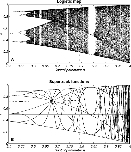
Figure 1: (A) Bifurcation diagram of the logistic map. (B) Low ordered supertrack functions $s_{i}(a)$ ($i=1\dots 10$) and the fixed point of the logistic map $1-1/a$ (dashed). Their intersections represent periodic windows, band merging and laminar states. The vertical dotted lines show a choosing of points of band merging and laminar behaviour ($a=3.678$, $3.727$, $3.752$, $3.791$, $3.877$, $3.927$).

A useful tool for studying the chaotic behavior are the recursively formed supertrack functions

$$s_{i+1}(a)=a\,s_{i}(a)\bigl{(}1-s_{i}(a)\bigr{)},\quad s_{0}(a)=\frac{1}{2}\,,$$ (6)

which represent the functional dependence of stable states Oblow (1988). The intersection of $s_{i}(a)$ with $s_{i+j}(a)$ indicates the occurrence of a $j$-period cycle and the intersection of $s_{i}(a)$ with the fixed-point $(1-1/a)$ of Eq. 5 indicates the point of an unstable singularity, i. e. laminar behavior (Fig. 1, intersection points are marked with dotted lines). For each $a$ we compute a time series of the length $N=2,000$. In order to exclude transient responses we use the last $1,000$ values of these data series in the following analysis.

We compute the RP after embedding the time series with a dimension of $m=1$, a delay of $\tau=1$ and a cut-off distance of $\varepsilon=0.1$ (in units of the standard deviation $\sigma$). Since the considered example is a one-dimensional map, $m=1$ is sufficient. In general, a too small embedding leads to false recurrences, which are expressed in numerous vertical structures and diagonals from the upper left to the lower right corner Gao and Cai (2000). In contrast, an over-embedding should theoretically not distort the reconstructed phase trajectory. Whereas false recurrences and over-embedding do not strongly influence the measures based on diagonal structures Gao and Cai (2000), the measures based on vertical structures are, in general, much more sensitive to the embedding. This is due to the fact, that the embedding method causes higher order correlations in the phase-space trajectory, which will be of course visible in the RP. A theoretical and more detailed explanation of this effect within the analysis of RPs is in preparation and beyond the scope of this article. For the logistic map, however, an increasing of $m$ slightly amplifies the peaks of the vertical based complexity measures (up to $m=3$), but it does not change the result significantly. The cut-off distance $\varepsilon$ is selected to be 10 percent of the diameter of the reconstructed phase space. Smaller values would lead to a better distinction of small variations (e. g. the range before the accumulation point consists of small variations). However, the recurrence point density decreases in the same way and thus the statistics of continuous structures in the RP becomes soon insufficient. Larger values cause a higher recurrence point density, but a lower sensitivity to small variations.

IV.1 Recurrence Plots of the Logistic Map

For various values of the control parameter $a$ we obtain RPs, which already exhibit specific features (Fig. 2). Periodic states (e. g. in the periodic window of length three at $a=3.830$) cause continuous and periodic diagonal lines in the RP of a width of one. There are no vertical or horizontal lines (Fig. 2 A). Band merging points and other cross points of supertrack functions (e. g. $a=3.720$, Fig. 2 C) represent states with short laminar behavior and cause vertically and horizontally spread black areas in the RP. The band merging at $a=3.679$ causes frequent laminar states and therefore a lot of vertically and horizontally spread black areas in the RP (Fig. 2 B). Fully developed chaotic states ($a=4$) cause a rather homogeneous RP with numerous single points and rare short diagonal or vertical lines (Fig. 2 D).

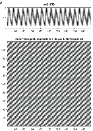
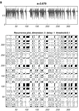
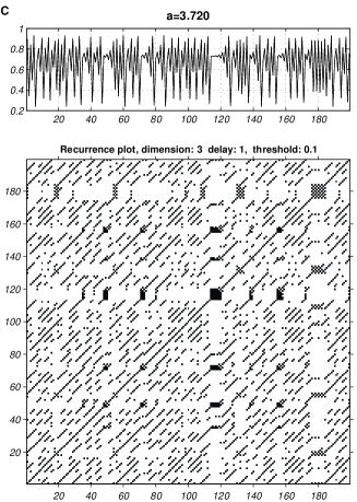
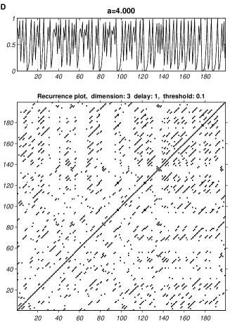
Figure 2: Recurrence Plots (RP) of the logistic map for various control parameters $a$, near different qualitative changes: periodic-3-window $a=3.830$ (A), band merging $a=3.679$ (B), supertrack intersection $a=3.720$ (C) and chaos (exterior crisis) $a=4$ (D); with embedding dimension $m=1$, time delay $\tau=1$ and distance cutoff $\varepsilon=0.1\sigma$.

IV.2 Complexity Measures of the Logistic Map

Now we compute the known RQA measures $\Delta$, $L_{max}$ and in addition $\langle L\rangle$ (average length of diagonal lines) and our measures $\Lambda$, $V_{max}$ and $T$ for the entire RP of each control parameter $a$. As expected, the known RQA measures $\Delta$, $L_{max}$ and $\langle L\rangle$ clearly detect the transitions from chaotic to periodic sequences and vice versa (Fig. 3 A, C, E) Trulla et al. (1996). However, it seems that one cannot get more information than the periodic-chaotic/ chaotic-periodic transitions. Near the supertrack crossing points (band merging points included), e. g. $a=3.678,3.791,3.927$, there are no significant indications in these RQA measures. They clearly identify the bifurcation points (periodic-chaotic/ chaotic-periodic transitions), without, however, finding the chaos-chaos transitions and the laminar states.

Calculating the vertical based measures $\Lambda$ and $T$, we are able to find the periodic-chaotic/ chaotic-periodic transitions and the laminar states (Fig. 3 B, F). The occurrence of vertical lines starts shortly before the band merging from two to one band at $a=3.678\dots$

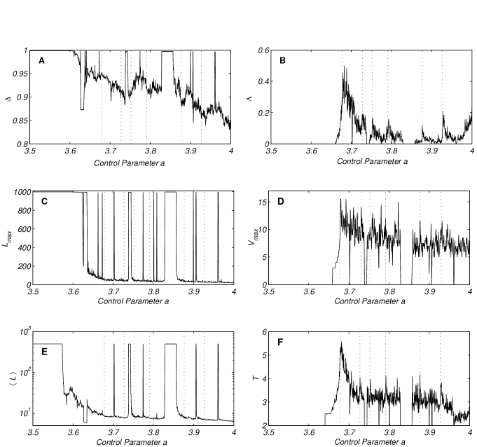
Figure 3: Selected RQA parameters $\Delta$, $L_{max}$ and $\langle L\rangle$ and the new measures $\Lambda$, $V_{max}$ and $T$. The vertical dotted lines show some of the points of band merging and laminar behavior (cf. Fig. 1), whereby not all of them have been marked. Whereas $\Delta$ (A), $L_{max}$ (C) and $\langle L\rangle$ (E) show periodic-chaotic/ chaotic-periodic transitions (maxima), $\Lambda$ (B), $V_{max}$ (D) and $T$ (F) exhibit in addition to those transitions (minima) chaotic-chaotic transitions (maxima). The differences between $\Lambda$ and $V_{max}$ are caused by the fact, that $\Lambda$ measures only the amount of laminar states, whereas $V_{max}$ measures the maximal duration of the laminar states. Although some peaks of $V_{max}$ and $T$ are not at the dotted lines, they correspond with laminar states (not all can be marked).

For smaller $a$-values the consecutive points jump between the two bands and it is therefore impossible to obtain a laminar behavior. A longer persistence of states is not possible until all bands are merged. However, due to the finite range of neighborhood searching in the phase space, vertical lines occur before this point.

Vertical lines occur much more frequently at supertrack crossing points (band merging points included), than in other chaotic regimes, which is revealed by $\Lambda$ (cf. Fig. 3 B, again, supertrack crossing points are marked with dotted lines). As in the states before the merging from two to one band, vertical lines are not found within periodic windows, e. g. $a=3.848$. The mean of the distribution of $v$ is the introduced measure $T$ (Fig. 3 F). It will vanish if $a$ is smaller than the point of merging from two to one band. $T$ increases at those points where more low ordered supertrack functions are crossing (Fig. 3 F). This corresponds to the occurrence of laminar states. Although $V_{max}$ also reveals laminar states, it is quite different from the other two measures, because it gives the maximum of all of the durations of the laminar states. However, periodic states are also associated with vanishing $T$ and $V_{max}$.

Hence, the vertical length based measures yield periodic-chaotic/ chaotic-periodic as well as chaos-chaos transitions (laminar states).

We have also computed $\Lambda$, $V_{max}$ and $T$ for the logistic map with transients using the same approach as described in Trulla et al. (1996). The qualitative statement of the measures is the same as above.

V Application to heart rate variability data

Heart rate variability (HRV) typically shows a complex behavior and it is difficult to identify disease specific patterns Schumann et al. (2002, in press). A fundamental challenge in cardiology is to find early signs of ventricular tachyarrhythmias (VT) in patients with an implanted cardioverter-defibrillator (ICD) based on HRV data Diaz et al. (2001); Huikuri and Makikallio (2001); Wessel et al. (2000b); Guzzetti et al. (2001). Therefore standard HRV parameters from time and frequency domain Task Force Heart Rate Variability (1996), parameters from symbolic dynamics Kurths et al. (1995); Voss et al. (1996) as well as the finite-time growth rates Nese (1989) were applied to the data of a clinical pilot study Wessel et al. (2000b). Using two nonlinear approaches, we have recently found significant differences between control and VT time series based mainly on laminar phases in the data before a VT. Therefore the aim of this investigation is to test whether our RP approach is suitable to identify and quantify these laminar phases.

The defibrillators used in the study cited (PCD 7220/7221, Medtronic) are able to store at least 1000 beat-to-beat intervals prior to the onset of VT (10 ms resolution), corresponding to approximately 9–15 minutes. We reanalyze these intervals from 17 chronic heart failure ICD patients just before the onset of a VT and at a control time, i. e. without a following arrhythmic event. Time series including more than one non-sustained VT, with induced VT’s, pacemaker activity or more than 10 % of ventricular premature beats are not considered in this analysis. Some patients had several VT’s; we finally had 24 time series with a subsequent VT and the respective 24 control series without a life-threatening arrhythmia. In order to analyze only the dynamics occurring just before a VT, the beat-to-beat intervals of the VT itself at the end of the time series are removed from the tachograms.

We calculate all standard RQA parameters described in Webber Jr. and Zbilut (1994) as well as the new measures laminarity $\Lambda$, trapping time $T$ and maximal vertical line length $V_{max}$ (in similarity to the maximal diagonal line length $L_{max}$) for different embedding dimensions $m$ and nearest neighbouring radii $\varepsilon$. We find differences between both groups of data for several of the parameters mentioned above. However, the most significant parameters are $V_{max}$ and $L_{max}$ for rather large radii (Tab. 1). The vertical line length $V_{max}$ is more powerful in discriminating both groups than the diagonal line length $L_{max}$, as can be recognized by the higher $p$-values for $V_{max}$ (Tab. 1). Figure 4 gives a typical example of the recurrence plots before a VT and at a control time with an embedding of 6 and a radius of 110. The RP before a life-threatening arrhythmia is characterized by large black rectangles ($V_{max}=242$ here), whereas the RP from the control series shows only small rectangles ($V_{max}=117$).

         

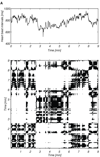
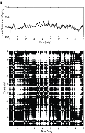
Figure 4: Recurrence plots of the heart beat interval time series at a control time (A) and before a VT (B) with an embedding of 6 and a radius of 110. The RP before a life-threatening arrhythmia is characterized by big black rectangles whereas the RP from the control series shows only small rectangles.

Table 1: Results of maximal diagonal and vertical line length shortly before VT and at control time, nonparametric Mann-Whitney U-test, $p$ – significance; * – $p<0.05$; ** – $p<0.01$; n. s. – not significant $p\geq 0.05$)

$m$	$\varepsilon$	VT	Control	$p$
Maximal diagonal line length $L_{max}$
$3$	$77$	396.6$\pm$253.8	261.5$\pm$156.6	n. s.
$6$	$110$	447.6$\pm$269.1	285.5$\pm$160.4	*
$9$	$150$	504.6$\pm$265.9	311.6$\pm$157.2	*
$12$	$170$	520.7$\pm$268.8	324.7$\pm$180.2	*
Maximal vertical line length $V_{max}$
$3$	$77$	261.4$\pm$193.5	169.2$\pm$135.9	*
$6$	$110$	283.7$\pm$190.4	179.5$\pm$134.1	**
$9$	$150$	342.4$\pm$193.6	216.1$\pm$137.1	**
$12$	$170$	353.5$\pm$221.4	215.1$\pm$138.6	**

VI Summary

We have introduced three new recurrence plot (RP) based measures of complexity, the laminarity $\Lambda$, the trapping time $T$ and the maximal length of vertical structures in the RP $V_{max}$. These measures of complexity have been applied to the logistic map and heart rate variability data. In contrast to the known RQA measures (Trulla et al. (1996), Zbilut and Webber Jr. (1992)), which are able to detect transitions between chaotic and periodic states (and vice versa), our new measures enable us to identify laminar states too, i. e. chaos-chaos transitions. These measures are provided by the vertical lines in recurrence plots. The occurrence of vertical (and horizontal) structures is directly related to the occurrence of laminar states.

The laminarity $\Lambda$ enables us generally to detect laminar states in a dynamical system. The trapping time $T$ contains information about the frequency of the laminar states and their lengths. The maximal length $V_{max}$ reveals information about the time duration of the laminar states thus making the investigation of intermittency possible.

If the embedding of the data is too small, it will lead to false recurrences, which is expressed in numerous vertical structures and diagonals perpendicular to the main diagonal. Whereas false recurrences do not influence the measures based on diagonal structures, the measures based on vertical structures are sensitive to it.

The application of these measures to the logistic equation for a range of various control parameters has revealed points of laminar states without any additional knowledge about the characteristic parameters or dynamical behavior of the specific systems. Nevertheless, $\Lambda$, $V_{max}$ and $T$ are different in their magnitudes. Further investigations are necessary to understand all relations between the magnitudes of $V_{max}$ and the recognized chaos-chaos transitions.

The application of the new complexity measures to the ICD stored heart rate data before the onset of a life-threatening arrhythmia seems to be very successful for the detection of laminar phases thus making a prediction of such VT possible. The differences between the VT and the control series are more significant than in Wessel et al. (2000b). However, two limitations of this study are the relative small number of time series and the reduced statistical analysis (no subdivisions concerning age, sex and heart disease). For this reason, our results should to be validated on a larger data base. Furthermore, this investigation could be enhanced for tachograms including more than 10% ventricular premature beats. In conclusion, this study has demonstrated that the RQA based complexity measures could play an important role in the prediction of VT events even in short term HRV time series.

Many biological data contain epochs of laminar states, which can be detected and quantified by the RP based measures. We have demonstrated differences between the measures based on the vertical and the diagonal structures and therefore we suggest the use of the method proposed in this article in addition to the traditional measures.

A download of the Matlab implementation is available at: www.agnld.uni-potsdam.de/~marwan.

VII Acknowledgments

This work was partly supported by the priority programme SPP 1097 of the German Science Foundation (DFG). We gratefully acknowledge M. Romano, M. Thiel and U. Schwarz for fruitful discussions.

References

- Glass (2001) L. Glass, Nature 410, 277 (2001).
- Blasius et al. (1999) B. Blasius, A. Huppert, and L. Stone, Nature 399, 354 (1999).
- Marvel (2001) K. B. Marvel, Nature 411, 252 (2001).
- Goldberger et al. (1988) A. L. Goldberger, D. R. Rigney, J. Mietus, E. M. Antman, and S. Greenwald, Experientia 44, 983 (1988).
- Glass and Kaplan (1993) L. Glass and D. Kaplan, Med. Prog. Technol. 19, 115 (1993).
- Abarbanel et al. (1993) H. D. I. Abarbanel, R. Brown, J. J. Sidorowich, and L. S. Tsimring, Rev. Mod. Phys. 65, 1331 (1993).
- Kantz and Schreiber (1997) H. Kantz and T. Schreiber, Nonlinear Time Series Analysis (University Press, Cambridge, 1997).
- Kurths and Herzel (1987) J. Kurths and H. Herzel, Physica D 25, 165 (1987).
- Mandelbrot (1982) B. B. Mandelbrot, The fractal geometry of nature (Freeman, San Francisco, 1982).
- Wolf et al. (1985) A. Wolf, J. B. Swift, H. L. Swinney, and J. A. Vastano, Physica D 16, 285 (1985).
- Wackerbauer et al. (1994) R. Wackerbauer, A. Witt, H. Atmanspacher, J. Kurths, and H. Scheingraber, Chaos, Solitons & Fractals 4, 133 (1994).
- Rapp et al. (2001) P. E. Rapp, C. J. Cellucci, K. E. Korslund, T. A. Watanabe, and M. A. Jimenez-Montano, Physical Review E 64, 016209 (2001).
- Kurths et al. (1995) J. Kurths, A. Voss, A. Witt, P. Saparin, H. J. Kleiner, and N. Wessel, Chaos 5, 88 (1995).
- Voss et al. (1996) A. Voss, J. Kurths, H. J. Kleiner, A. Witt, N. Wessel, P. Saparin, K. J. Osterziel, R. Schurath, and R. Dietz, Cardiovasc Res 31, 419 (1996).
- Wessel et al. (2000a) N. Wessel, A. Voss, J. Kurths, A. Schirdewan, K. Hnatkova, and M. Malik, Med Biol Eng Comput 38, 680 (2000a).
- Engbert et al. (1997) R. Engbert, M. S. C. Scheffczyk, J. Kurths, R. Krampe, R. Kliegl, and F. Drepper, Nonlin. Anal. Theo. Meth. Appl. 30, 973 (1997).
- Hempelmann and Kurths (1990) A. Hempelmann and J. Kurths, Astron. Astrophys. 232, 356 (1990).
- Schwarz et al. (1993) U. Schwarz, A. O. Benz, J. Kurths, and A. Witt, Astron. Astrophys. 277, 215 (1993).
- Witt et al. (1994) A. Witt, J. Kurths, F. Krause, and K. Fischer, Geoph. Astroph. Fluid Dyn. 77, 79 (1994).
- Casdagli (1997) M. C. Casdagli, Physica D 108, 12 (1997).
- Eckmann et al. (1987) J.-P. Eckmann, S. O. Kamphorst, and D. Ruelle, Europhysics Letters 5, 973 (1987).
- Koebbe and Mayer-Kress (1992) M. Koebbe and G. Mayer-Kress, in Proceedings of SFI Studies in the Science of Complexity. Nonlinear modeling and forecasting, edited by M. Casdagli and S. Eubank (Addison-Wesley, Redwood City, 1992), vol. XXI, pp. 361–378.
- Trulla et al. (1996) L. L. Trulla, A. Giuliani, J. P. Zbilut, and C. L. W. Jr., Physics Letters A 223, 255 (1996).
- Webber Jr. and Zbilut (1994) C. L. Webber Jr. and J. P. Zbilut, Journal of Applied Physiology 76, 965 (1994).
- Zbilut and Webber Jr. (1992) J. P. Zbilut and C. L. Webber Jr., Physics Letters A 171, 199 (1992).
- Wessel et al. (2000b) N. Wessel, C. Ziehmann, J. Kurths, U. Meyerfeldt, A. Schirdewan, and A. Voss, Physical Review E 61, 733 (2000b).
- Argyris et al. (1994) J. H. Argyris, G. Faust, and M. Haase, An Exploration of Chaos (North Holland, Amsterdam, 1994).
- Ott (1993) E. Ott, Chaos in Dynamical Systems (University Press, Cambridge, 1993).
- Gao (1999) J. B. Gao, Physical Review A 83, 3178 (1999).
- Gao and Cai (2000) J. B. Gao and H. Q. Cai, Physics Letters A 270, 75 (2000).
- Marwan (1999) N. Marwan, Master’s thesis, Dresden University of Technology, Dresden (1999).
- Collet and Eckmann (1980) P. Collet and J.-P. Eckmann, Iterated maps on the interval as dynamical systems (Birkhäuser, Basel Boston Stuttgart, 1980).
- Oblow (1988) E. M. Oblow, Phys. Lett. A 128, 406 (1988).
- Schumann et al. (2002, in press) A. Schumann, N. Wessel, A. Schirdewan, K. J. Osterziel, and A. Voss, Statist Med (2002, in press).
- Diaz et al. (2001) J. O. Diaz, T. H. Makikallio, H. V. Huikuri, G. Lopera, R. D. Mitrani, A. Castellanos, R. J. Myerburg, P. Rozo, F. Pava, and C. A. Morillo, Am J Cardiol 87, 1123 (2001).
- Huikuri and Makikallio (2001) H. V. Huikuri and T. H. Makikallio, Auton Neurosci 90, 95 (2001).
- Guzzetti et al. (2001) S. Guzzetti, R. Magatelli, E. Borroni, and S. Mezzetti, Auton Neurosci 90, 102 (2001).
- Task Force Heart Rate Variability (1996) Task Force Heart Rate Variability, Circulation 93, 1043 (1996).
- Nese (1989) J. M. Nese, Physica D 35, 237 (1989).