Helium in superstrong magnetic fields
Abstract
We investigate the helium atom embedded in a superstrong magnetic field - au. All effects due to the finite nuclear mass for vanishing pseudomomentum are taken into account. The influence and the magnitude of the different finite mass effects are analyzed and discussed. Within our full configuration interaction approach calculations are performed for the magnetic quantum numbers M=,,,, singlet and triplet states, as well as positive and negative z parities. Up to six excited states for each symmetry are studied. With increasing field strength the number of bound states decreases rapidly and we remain with a comparatively small number of bound states for au within the symmetries investigated here.
I Introduction
The term “strong” field characterizes a situation for which the system is in the nonperturbative regime, i.e. where the magnetic forces are of the same order of magnitude or greater than the Coulomb binding force. For the ground state of the hydrogen atom this corresponds to field strengths a.u. (1 a.u. corresponds to T). We refer to the term “superstrong” to indicate a field strength of atomic units and more.
The motivation to study atoms and molecules in strong magnetic fields originates from several sources. Certainly the properties of atoms and molecules in strong magnetic fields are interesting from a pure theoretical point of view. Due to the competition of the spherically symmetric Coulomb potential and the cylindrically symmetric magnetic field interaction we encounter a nonseparable, nonintegrable problem already for a one-electron system, i.e. the hydrogen atom. Therefore it is necessary to develop new techniques to solve the Schrödinger equation in strong magnetic fields.
The discovery of strong magnetic fields on the surface of magnetic white dwarfs (– T) and neutron stars (– T) is a further major motivation. The spectra of these astrophysical objects can be dominated by the influence of magnetic and electric fields. For the analysis of atmospheres of magnetic white dwarfs and neutron stars, it is very important to have reliable data on the behavior of matter in strong magnetic fields. As an example we mention the the white dwarf GrW+70∘. The interpretation of its spectrum was very important for the understanding of the properties of spectra of magnetic white dwarfs in general (see Refs. [1, 2, 3, 4, 5]).
Highly accurate data are available for hydrogen in strong magnetic fields (see e.g. [6, 7]). This system is now understood to a very high degree. But there is also a significant interest in accurate data on heavier elements such as He, Na, Fe and molecules. Especially helium plays an important role in the atmosphere of certain magnetic white dwarfs (see e.g. [8, 9, 10]).
There were several attempts to calculate accurate energies for bound states of helium, but for astrophysical applications an accuracy of approximately for the energies is needed for a large number of levels. We will concentrate here on investigations that address the high field regime: In 1975 Mueller et al. [11] calculated the few lowest levels of He for up to 20000 a.u. using a variational approach. Virtamo [12] presented Hartree-Fock calculations on the ground state (which is a triplet state with magnetic quantum number equal to ). The same state has been considered by Pröschl [13] in 1982 in the range 21 – 21000 au. Vincke and Baye [14] provide correlated calculations (=, and a.u.) for the lowest singlet and triplet states with positive z parity and magnetic quantum numbers =,,. In the work of Thurner [15] several triplet states are considered in the very broad range = — a.u. We mention also the important work by Becken and Schmelcher, which covers the same symmetries and the same number of excited states in the broad range — a.u. of the magnetic field strength published in a series of papers [16, 17, 18, 19].
The properties of matter in superstrong magnetic fields are especially interesting for the physics of cold neutron stars [20, 21, 22]. But for the case of superstrong magnetic fields the finite nuclear mass effects become increasingly important. This is due to the fact, that energy shifts, caused by the finite nuclear mass, are of the order of , where is the mass of the nucleus. Evidently this correction is for superstrong magnetic fields of the same order of magnitude as the ionization energies.
Of course the conceptual and in particular the computational situation becomes more complex when the full Hamiltonian, i.e. for finite nuclear mass, is taken into account. For both neutral [23, 24] as well as charged systems [23, 24, 25, 26, 27, 28, 29, 30, 31, 32] we encounter couplings among the different electrons as well as couplings between the collective and electronic motion.
Some approximations to the ionic problem are available: An approximate separation of the collective and relative motion of the charged system has been introduced in [25] and applied to calculate the finite nuclear mass corrections for low-lying levels of hydrogenic ions in a magnetic field [26]. Elaborated MCHF computations as well as adiabatic approximations were given in Ref. [32]. However these approaches cannot be used to calculate accurate results for all field strengths and all states investigated here. We mention that the behavior of the ion He+ has to be known in order to determine the ionization energies of the neutral He atom.
In the present paper we provide a full configuration interaction calculation for helium in superstrong magnetic fields. All finite mass effects at zero pseudomomentum are taken into account and are analyzed. In section II we will describe the Hamiltonian, and some technical details concerning our calculation. Furthermore we provide some remarks on the problem of the threshold energies. In section III we analyze the deviations of the Hamiltonian in the infinite nuclear mass frame from the full Hamiltonian. Ionization energies and transition wavelengths, resulting from our calculations, are provided in Sect. IV.
II Formulation of the problem
A Hamiltonian and Symmetries
To investigate the He atom we use a nonrelativistic approach. This is well justified by the fact, that relativistic corrections have been shown to be very small in strong and even superstrong magnetic fields [33, 34]. For the sake of simplicity we take the electronic spin g factor to be 2, but our results can be easily adapted to any g factor by multiplying the spin operators and their eigenvalues by . On the other hand, the ionization energies, and transition wavelengths, which are presented in this paper are not affected by this choice. The magnetic field vector will be denoted by , whereas its magnitude will be denoted by . The magnetic field vector is chosen to point in z direction.
The first step in our approach is the pseudoseparation of the collective and relative motion for the Hamiltonian in the laboratory frame [23, 24, 35] which exploits the conservation of the so-called pseudomomentum . The resulting transformed Hamiltonian is divided into three parts, which are denoted by , , and . The operator involves only center of mass (CM) degrees of freedom, where is the mass of the atom. contains exclusively electronic degrees of freedom. The operator represents the coupling between and , i.e. the CM and electronic degrees of freedom. It involves the motional electric field which arises due to the motion of the (neutral) atom in the magnetic field and is oriented perpendicular to the magnetic field. This coupling is proportional to the pseudomomentum, and therefore vanishes for vanishing pseudomomentum. The pseudoseparation is possible for neutral systems only, since only then all components of the pseudomomentum commute.
Within the present work we assume a vanishing pseudomomentum. Therefore we have no additional motional electric field and all effects due to the finite nuclear mass are included in which is a function of the mass of the nucleus and the magnetic field . In atomic units the electronic Hamiltonian takes the following form (internal coordinates are taken with respect to the nucleus):
| (1) |
where
| (3) | |||||
and
| (4) |
The reduced masses are and . The Hamiltonian can be considered to consist of three parts. The first part contains the one-particle operators , the Zeeman terms , the diamagnetic terms , the attractive Coulomb interaction with the nucleus , and the spin Zeeman terms . The second part contains the two particle operator (3), which describes the repulsive Coulomb interaction between the two electrons. The third operator is the so-called mass polarization operator . It arises due to the transformation of the laboratory coordinates to the internal coordinates, which are relative to the nucleus. The reader should note that the Hamiltonian (1) has the same good quantum numbers as the Hamiltonian for infinite nuclear mass: the total spin , the z component of the total spin, the magnetic quantum number and the total spatial z parity (parity is not an independent symmetry, it can be deduced from these corresponding symmetry operations). In the following we will denote the states by , where is the spin multiplicity and denotes the degree of excitation within a given subspace.
If we compare in Eq. (1) to the electronic Hamiltonian of helium in the infinite nuclear mass frame [16] , we observe two different kinds of corrections due to the finite nuclear mass. The first is due to the occurrence of the reduced masses and in which are the so called normal mass corrections. The spectrum of the Hamiltonian which contains exclusively these normal mass corrections can be related to the spectrum of the Hamiltonian at a different field strength , via a unitarian transformation and an additional trivial energy shift (see section III and also Refs. [6, 16, 36]). The second type of finite nuclear mass effects is due to the mass polarization operators . We will call these specific finite mass corrections. They are by no means trivial and are related to the correlation of the electrons (the corresponding operators contain one-particle operators of both electrons). If the electrons behave in a correlated way, the specific nuclear mass effects are enhanced. Note that these operators are a consequence of the transformation from the laboratory to our non-inertial system thereby eliminating the CM degrees of freedom.
B Technical remarks
Some comments concerning our computational approach are in order. Its basic ingredient is an anisotropic Gaussian basis set, which was put forward by Schmelcher and Cederbaum [37]. This one-particle basis is sufficiently flexible to to describe finite electronic systems for any field strength and was successfully applied to several atoms and molecules in magnetic fields [16, 17, 18, 38, 39, 40, 41].
This basis set is not only flexible: in the case of atoms all matrix element can be calculated analytically and in particular evaluated efficiently [16, 17]. The price, which has to be paid, is that for each field strength and each symmetry, the basis set has to be (nonlinearly) optimized. This is achieved by variationally computing the eigenfunctions of the corresponding one-particle problems (H, He+, etc). This task is time consuming and needs experience, because the starting values for the nonlinear variational parameters have to be chosen carefully in oder to obtain well-converged results. In recent times however this has become more comfortable and was speeded up by new optimization algorithms and tools, which allow an almost automatic construction of a basis set. The implementation of these tools still needs a proper selection of the coefficients and an evaluation of the outcome of the optimization. The latter is of particular importance for the field regime addressed in the present work for which small changes in the basis set can have a considerable effect on the results of the full problem, i.e. the eigenenergies and eigenfunctions of in Eq. (1). A one particle basis set typically consists of 200–400 basis functions, which combine 3000 to 5000 two particle configurations. The full CI approach leads then to a generalized eigenvalue problem. Numerical problems arise in this generalized eigenvalue problem if near linear dependencies in the basis set arise. These dependencies cannot fully be avoided, but the resulting numerical instabilities can be removed by a cutoff of the small eigenvalues of the corresponding overlap matrix.
The most CPU time consuming part in the above approach, is the evaluation of the electron-electron matrix elements. Although analytical formulas for all matrix elements are available, it is important to have efficient algorithms for their evaluation, since the matrix elements for the electron-electron Coulomb interaction are by no means trivial. A detailed and sophisticated analysis of their analytical representation is crucial. In the simplest form it contains multiple sums over hypergeometric functions [16, 17]. For the evaluation of the hypergeometric function all possible analytical continuation formulas have been worked out (see Ref. [42]) and made it possible to reduce the time for the calculation of the matrix elements by a factor of 50 compared to a straightforward implementation. We emphasize that the present investigation would have been impossible without this efficient implementation of the evaluation of the matrix elements.
C Threshold
The result of the solution of the generalized eigenvalue problem are the total energies of the system. These energies are however not of primary interest: they increase almost linearly with the magnetic field strength due to the raise of the kinetic energy in the presence of the field. The relevant energies are e.g. the transition and ionization energies which are for the high field regime addressed here by several orders of magnitude smaller than the total energies and therefore ‘hidden’ in the total energies. To obtain the ionization energies we need to know the energy of the He+ ion taking into account the finite nuclear mass in the magnetic field. These energies for He+ are unfortunately not known exactly. In contrast to this the energies for He+ assuming an infinite nuclear mass can be calculated from the well-known energies for the hydrogen atom with fixed nucleus in strong magnetic fields (see e.g. Ref.[7]) via the corresponding scaling relations (see for example [6]). However the energies of the He+ ion with finite nuclear mass cannot be extracted from results for the hydrogen atom (with finite or infinite nuclear mass) because of the unique coupling between the collective and electronic motion which has to be taken into account. This coupling inherently mixes the collective and electronic motion and the exact ground state therefore combines both motions. The moving He+–ion in a strong magnetic field is a problem which has not been solved numerically exactly in the literature. As a result the exact threshold energy for He+ + e- is not known. Using the threshold energy of He+ + e- for fixed nucleus E provides a wrong description of the threshold energies in superstrong fields.
The Hamiltonian for the helium positive ion reads in atomic units as follows:
| (5) | |||||
| (6) | |||||
| (7) | |||||
| (8) |
Here describes the collective motion of the ion as a free particle with charge 1 and mass moving in a magnetic field ( and are the center of mass coordinate and momentum, respectively). The operator couples electronic and collective motion. The operator is the electronic part of the He+ Hamiltonian with and .
Although the exact threshold energy for He+ + e- is not available some approximations to it have been calculated in the literature. One of those approximations E ignores the coupling between the collective and electronic motion . The corresponding threshold values consist of the sum of eigenenergies of the electronic Hamiltonian and the zero point energy for . The zero point energy for the collective motion is the corresponding energy for the lowest Landau level. The energy for this threshold is typically too high, i.e. the true ionization energies are overestimated, since the coupling , which is neglected in this approximation, tends to reduce the threshold energy. All ionization energies shown in the present work are calculated by applying E.
The second approximation we will choose, ignores the zero point energy of the ion and the coupling term, i.e. and . Therefore, only the eigenenergies of the mass corrected electronic Hamiltonian are taken into account. This threshold is denoted as E. It is motivated by the fact, that for an infinitely strong magnetic field the energetic contributions due to the zero point energy of and the coupling exactly cancel. A third alternative threshold energy E is obtained by employing the adiabatic expansion approach presented in [32]. Since this approximation only takes into account the lowest Landau energy for the CM motion, it becomes increasingly accurate for increasing energetic separation between the Landau levels (and therefore increasing magnetic field strength). For field strengths below a.u. this approximation is not reliable. It can be observed, that the threshold E approaches the threshold energy E in the limit of high fields. E is expected to be very accurate for sufficient high field strengths.
III The finite nuclear mass effects
There is a transformation, which connects the spectrum of the infinite nuclear mass Hamiltonian with the spectrum of the Hamiltonian Hrm [16]. This transformation reads as follows:
| (9) |
Here denotes a unitarian transformation, which transforms and . The second term on the right hand side of Eq. (9) represents a field dependent trivial energy shift, since the total z component of the spin and the total z component of the orbital angular momentum are conserved quantities.
From equation (9) it can be seen, that the leading mass correction is of the order of . For the states with magnetic quantum number , this correction is positive. This means that the corresponding energy levels are shifted i.e. increase linearly with and eventually pass the ionization threshold. The latter implies that the corresponding bound electronic state becomes ionized. This shift depends exclusively on the magnetic quantum number , the total z component of the spin , the magnetic field strength , and the nuclear mass M0.
The energy difference =EE, where denotes the eigenvalues of and the eigenvalues of , can be related to the energy difference of the eigenvalues of the Hamiltonian H and H. The operator H describes two free noninteracting electrons
| (10) |
whereas H refers to the corresponding ‘artificial’ Hamiltonian with reduced masses
| (11) |
For the energetically lowest Landau level with negative magnetic quantum number and vanishing momentum in z direction we have
| (12) |
It cannot be expected, that the normal mass corrections of the helium atom follow exactly equation (12), because the Hamiltonian Hrm contains the interaction between the two electrons and of the electrons with the nucleus. However it is suggestive to introduce a parameter such that
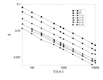
For the states and field strengths investigated in the present work we have . Therefore can be treated as a correction term. Since this correction is due to the Coulomb interaction it is state dependent. In Fig. 1 the quantity is shown as a function of the magnetic field strength for a few selected singlet states belonging to several different symmetries. It can be seen, that , for all states considered, follows a power law , where the exponent does not depend on the state. However the corresponding proportionality constant varies over nearly one order of magnitude for the different states.
To understand more on the behavior of the quantity we expand the first part on the right hand side of Eq. (9) in powers of . Omitting the spin part we obtain:
| (13) | |||||
| (14) |
Here the prime indicates the derivative with respect to the field strength. Now and consequently can be expressed in terms of the eigenenergies of H():
| (15) |
Now the state dependency of can be understood as the dependence on the derivative of the eigenenergies with respect to the field strength. We emphasize, that the quantities and in Eq. (15) are almost equal and therefore approximately cancel in the superstrong field regime. Thus can be approximated by .
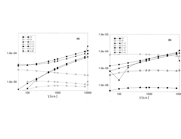
Fig. 2 (a) illustrates the mass polarization energies for the energetically lowest singlet states and Fig. 2 (b) for the corresponding triplet states. Here denotes the eigenenergies of . First we observe, that the absolute values of are very small: For they are at least eight orders of magnitude smaller than the corresponding total energies. They are also small compared to the normal finite mass corrections . For is at least four orders of magnitude smaller the normal finite mass corrections. Opposite to the quantity the behavior of depends strongly on the state. For the states ,,, the quantity increases. These states contain so-called magnetically tightly bound orbitals [6, 43, 44] and therefore their ionization energy diverges logarithmically in the limit . An increase of the influence of can also be observed in Fig. 2 (b) for the states , and , which represent also magnetically tightly bound states. For the remaining states , and the corresponding triplet states as well for remains almost constant as a function of the magnetic field strength. This effect can be easily understood: For the magnetically tightly bound states the electrons are close to each other in a relatively narrow region of space and therefore electron correlation is important. The mass polarization operator is sensitive to electronic correlation, due to the fact that it contains operators of both electrons. The sign of is not shown in Fig. 2. It is positive for the states related to the above mentioned tightly bound states and negative for the others. The only exception is the state , which does not belong to the tightly bound states, but nevertheless has a positive sign.
IV Results
In the following we will present our results for the ionization energies and transition wavelengths of the helium atom for magnetic fields ranging from au to au. These investigations have been performed for the magnetic quantum numbers , singlet and triplet states and positive and negative z parity. Only for the magnetic quantum number exclusively positive z parity states have been studied. For most symmetry subspaces we investigated 6 excited states.
A Ionization energies
According to the above the reader should keep in mind, that the exact energy of the ionization threshold is not known, and therefore the ionization energies are not known accurately. However the ionization energies calculated by using different approximative threshold energies , , , show the same trend: the number of bound states of the helium atom becomes finite for superstrong magnetic fields in contrast to the situation without a magnetic field, or in the limit of an infinitely heavy nucleus, where the helium atom has an infinite number of bound states. Only the so-called magnetically tightly bound states are bound within the complete regime of field strengths and quantum numbers considered in the present work. We consider in the following the quantity as a function of the field strength together with the above mentioned approximations for the threshold.
Fig. 3 (a) shows for the six energetically lowest states of zero magnetic quantum number and positive z parity. The state is the most tightly bound state. In strong magnetic fields it represents however not the ground state of the atom, because energetically low-lying states are fully spin-polarized in the high field regime. The ground state is given by the state, which is also a tightly bound state. Fig. 3 (a) shows, that increases for the tightly bound state , but remains approximately constant for all other states as a function of the magnetic field strength. Furthermore we observe that all states with as well as the corresponding triplet states pass the threshold energies being either or with increasing field strength. The only remaining bound state for au is the state.
In Fig. 3 (b) the corresponding quantity for states with and negative z parity are shown. For these states as a function of varies only to a very minor extent, which is due to the fact, that none of these states is a tightly bound one, and none of these states remains bound when approaches au. For the triplet states with negative z parity the quantity decreases slightly, for au. This is not due to the finite mass effect, but can be also observed for the quantity , whereas this quantity increases monotonically for all other states investigated in the present work. The reason is the complicated interplay between correlation, which tends to increase ionization energies and Coulomb repulsion, which tends to decrease it. For the states with the electrons are confined in a very small domain of space, which increases correlation as well as the Coulomb repulsion. On the other hand for triplet states the electrons are separated, because the wavefunction is antisymmetric, which reduces both effects. For the states the increase of correlation energy is smaller than the increase of the Coulomb repulsion energy.
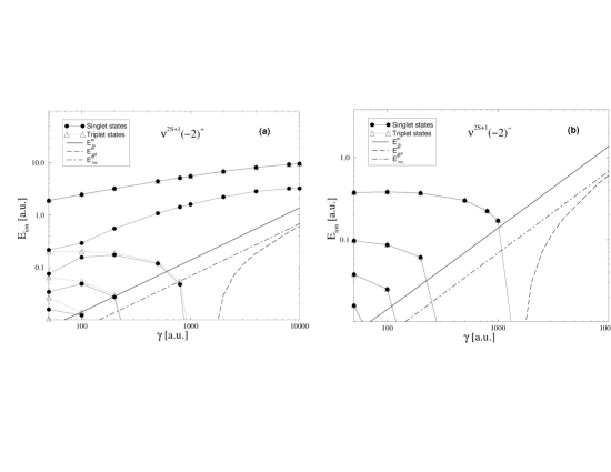
In figure 4 (a) is shown for the states . For the magnetically tightly bound states and the ionization energy remains positive, i.e. these states are bound in the complete regime au. For higher excited states, i.e. with the energy becomes even larger than and therefore decreases strongly on the logarithmic scale. To understand this we review Eq. (9): The dominant term on the right hand side is of the form (the spin part does not affect the ionization energies). Therefore for states with raises about this amount and will pass the threshold at lower field strength than their counterparts with .
In Fig. 4 (b) we show our results for for and negative z parity. A similar behavior to that of the states , with is observed: The ionization energy as a function of the magnetic field strength decreases rapidly. This is due to the fact, as mentioned above, that the finite mass corrections force these states to pass even the threshold and the states become unbound. For negative z parity tightly bound states do not exist.
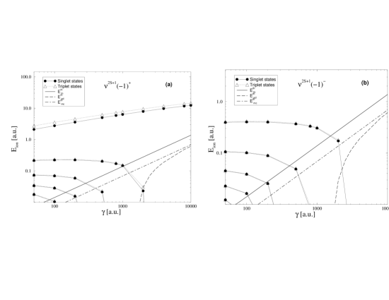
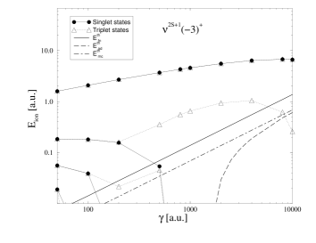
In Fig. 5 (a) we present our results for for the energetically lowest singlet and triplet states with and positive z parity. Similar to Fig. 4 (a) the quantity rises for the two energetically lowest singlet and triplet states from au to approximately 10 au. These two states belong to the magnetically tightly bound states. However in contrast to for the states in Fig. 4 (a) for the state , which is the first excited singlet state of this symmetry, does also rise and stays bound within the complete regime of field strength considered here. This is a remarkable feature since the influence of the finite mass effects for this state is even bigger than for the states with . The reason for this behavior lies in the presence of an avoided crossing which takes place at au. It can be seen that for the higher excited singlet states is raised as well and it approaches the corresponding value for the next energetically higher triplet state.
The ionization energies for the negative z parity states for in Fig. 5 (b) look similar to these of the in Fig. 4 (b). Magnetically tightly bound states do not exist for and negative parity, therefore all states of this symmetry become unbound with increasing field strength. As mentioned above the influence of the finite nuclear mass increases with increasing magnetic quantum number , therefore the states become unbound at lower field strengths than the corresponding states with magnetic quantum number .
In Fig. 6 we encounter that for the energetically lowest singlet and triplet states with and positive z parity is positive for all field strengths, considered in the present work. These two states belong to the magnetically tightly bound states. Similar to Fig. 5 (a) an avoid crossing takes place at au. This can be more clearly seen if the quantity is considered. But unlike to the case of , where Eion for the first excited singlet state is raised, here the triplet state is shifted to lower energies and remains therefore bound for relatively high field strengths. Nevertheless, the state passes the ionization threshold for approaching au and therefore becomes unbound due to the influence of the finite nuclear mass effects.
B Transition wavelengths
In contrast to the ionization energies, which strongly depend on the exact values for the threshold energies, transition wavelengths can be calculated from total energies without the knowledge of the exact threshold energy. The only feature which remains unknown for the transition wavelengths is the exact field strength, foe which the particular bound-bound transition disappears. Therefore we refer the total energy of a state to the threshold in order to decide upon its bound character as a function of the field strength. According to the discussion provided in Sect. II C the true field strength for which the state becomes unbound is lower than the value obtained by refering the total energies to .
Some general remarks on our results for the transition wavelengths presented in Figs. 7 – 14 are in order. Linearly polarized transitions show the general feature, that there are two separated parts of the spectrum. A few transition wavelengths become shorter, following approximately a power law as a function of the field strength. Other transition wavelengths, which are much longer, stay almost constant as a function of the magnetic field strength. The short wavelengths correspond to transitions involving the magnetically tightly bound states. The other lines correspond to transitions between higher excited states.
For circular polarized transitions the appearance of the spectrum of wavelengths is different. Only for circular polarized transitions which involve states with positive z parity a separated bundle of short wavelengths is present. This is again due to the presence of tightly bound states for positive z parity but their absence for negative z parity states. Transitions between higher excited states which do not involve tightly bound states, look different than their corresponding linear polarized transitions: the wavelengths increase or decrease as a function of . In the case of circular polarized transitions, states belonging to different magnetic quantum numbers are involved and therefore the energy of the state with the higher absolute value of the magnetic quantum number raises more strongly with increasing field strength than the energy of the state with the lower magnetic quantum number. This again goes back to the nuclear mass effects contained in Eq. (9) and yields the increase or decrease of the wavelengths for the circular polarized transitions with increasing field strengths.
In Fig. 7 the transition wavelengths for the singlet and triplet transitions among the and states are shown. The separation mentioned above, which is a general feature for linearly polarized transitions is obvious. The short wavelengths are the transitions involving the most tightly bound state . According to Fig. 3 (a) its ionization energy increases with increasing field strength, whereas the ionization energy of all other (excited) states varies only marginally.
The circular polarized transition wavelengths shown in Fig. 8 involve the and symmetry subspaces. Separated by a large energetically gap there is a bundle of short wavelengths, which is due to transitions to the magnetically tightly bound states , and and a long wavelength part.
The spectrum of circular polarized transitions among the subspaces and , shown in Fig. 9 shows also the characteristics of circular polarized transitions discussed above. Since in this case only states with negative z parity are involved, we have no tightly bound states,and the part of the spectrum with very short wavelengths is missing.
The behavior of the wavelengths of the linear polarized transition from the states to the states is shown in Fig. 10 and looks similar to the one given in Fig. 7. Two well separated parts of the spectrum can be distinguished: Short wavelengths, which are due to transitions to the magnetically tightly bound states and and decrease as a function of the field strength. Transition wavelengths between higher excited states, with wavelengths larger than 1000 Ångstrøm, remain approximately constant. Due to the fact, that the influence of the finite nuclear mass is more significant than for those shown in Fig. 7, much less lines belonging to bound-bound transitions are present.
The spectrum shown in Fig. 11 for the symmetry subspaces and differs in some respect from the common pattern of circularly polarized transitions. Similar to other spectra circular polarized transitions, wavelengths involving transitions to the tightly bound states (,,,) can be easily identified. As a function of the magnetic field strength, these wavelengths follow approximatively a power law. On the other hand there are structures shown in Fig. 11, which arise due to the influence of the finite nuclear mass. However in the gap between these two parts of the spectrum, additional lines occur which are caused by avoided crossings. The transitions to shown in Fig. 12 show the clear signature described above for circular polarized transitions. Only a few lines belong to bound-bound transitions.
The spectral transitions given in Fig. 13 ( to ) show the typical behavior of linear polarized transitions. Deviating from the general pattern, transition wavelengths to the state form their own bundle of short wavelengths, being located between the wavelengths of the transitions of the tightly bound states and and the transitions among higher excited states.
The spectrum of transitions among the subspaces to is shown in Fig. 14. Transitions to the magnetically tightly bound states ,, , can be clearly identified. Also the transitions dominated by the normal finite mass effects can be seen for long wavelengths. Additionally the influence of the avoided crossings is visible.
V Brief Summary
We have presented the first systematic full CI calculations for helium in superstrong magnetic fields, taking into account the effects of finite nuclear mass. These effects are extremely important in the superstrong field regime, because the relevant parameter for the importance of the finite nuclear mass effects is . We analyzed the influence of the normal and the specific finite nuclear mass effects. It has been shown that the leading finite nuclear mass effect, does not depend on the state, but only on the magnetic quantum number. The state dependent part of the normal finite mass effects depends on the derivative with respect to the magnetic field strength of the total energy of the corresponding state in the infinite nuclear mass frame. Furthermore it has been shown, that the specific mass effects, which are caused by the mass polarization operators, are very small compared to the total energies and small compared to the leading normal mass effects .
In the superstrong magnetic field regime, the spectrum of helium is cut off by the effects of the finite nuclear mass. We found that only a comparatively small number of
states is bound in the complete regime of magnetic field strengths investigated in the present work. Although the exact ionization threshold for helium is unknown, all available approximations to the exact threshold confirm this trend. Transition wavelengths for many linear and circular polarized transitions were provided. Their typical behavior has been identified and the effects of the finite mass on the transition wavelengths has been analyzed.
The determination of the critical field strengths (i.e. the field strengths where the individual states become unbound) require a detailed investigation of the ground state of the moving helium positive ion in a magnetic field.
Acknowledgments
The Deutsche Forschungsgemeinschaft (O.A.A.) is gratefully acknowledged for financial support.


REFERENCES
- [1] J. Angel, J. Liebert, and H. S. Stockmann, Astrophys. J. 292, 260 (1985).
- [2] J. Angel, Ann. Rev. Astron. Astrophys. 16, 487 (1978).
- [3] J. L. Greenstein, R. Henry, and R. F. O‘Connel, Astrophys. J. 289, L25 (1985).
- [4] G. Wunner, W. Rösner, H. Herold, and H. Ruder, Astron. Astrophys. 149, 102 (1985).
- [5] D. T. Wickramasinghe and L. Ferrario, Astrophys. J. 327, 222 (1988).
- [6] H. Ruder, G. Wunner, H. Herold, and F. Geyer, Atoms in strong magnetic fields (Springer Verlag, Berlin, 1994).
- [7] Y. P. Kravchenko, M. A. Liberman, and B. Johansson, Phys. Rev. A 54, 287 (1996).
- [8] S. Jordan, P. Schmelcher, W. Becken, and W. Schweizer, Astron. Astrophys. Lett. 336, L33 (1998).
- [9] S. Jordan, P. Schmelcher, and W. Becken, Astron. Astrophys. 376, 614 (2001).
- [10] D. T. Wickramasinghe and L. Ferrario, Pub. Astron. Soc. Pac. 112, 873 (2000).
- [11] R. O. Mueller, A. Rau, and L. Spruch, Phys. Rev. A 11, 789 (1975).
- [12] J. Virtamo, J. Phys. B 9, 751 (1976).
- [13] P. Pröschl, W. Rösner, G. Wunner, and H. Herold, J. Phys. B 15, 1959 (1982).
- [14] M. Vincke and D. Baye, J. Phys. B 22, 2089 (1989).
- [15] G. Thurner et al., J. Phys. B 26, 4719 (1993).
- [16] W. Becken, P. Schmelcher, and F. Diakonos, J. Phys. B 32, 1557 (1999).
- [17] W. Becken and P. Schmelcher, J. Phys. B 33, 545 (2000).
- [18] W. Becken and P. Schmelcher, Phys. Rev. A 63, 053412 (2001).
- [19] W. Becken and P. Schmelcher, acc. f. publ. in Phys. Rev. A, (2001).
- [20] G. G. Pavlov and A. Y. Potekhin, Astroph. J. 450, 883 (1995).
- [21] G. G. Pavlov, Y. A. Shibanov, V. E. Zavlin, and R. D. Meyer, in Proc. NATO ASI C 450, edited by M. A. Alpar, U. Kiziloǧlu, and J. van Paradijs (Kluwer, Dordrecht, 1995), pp. 71–90.
- [22] J. H. Taylor, R. N. Manchester, and A. G. Lyne, Astrophys. J. Suppl. Ser. 88, 529 (1993).
- [23] P. Schmelcher, L. S. Cederbaum, and U. Kappes, in Conceptual Trends in Quantum Chemistry, edited by E. S. Kryachko and J. L. Calais (Kluwer, Dordrecht, 1994), pp. 1–51.
- [24] B. R. Johnson, J. O. Hirschfelder, and K. H. Yang, Rev. Mod. Phys. 55, 109 (1983).
- [25] D. Baye, J. Phys. B 15, L795 (1982).
- [26] D. Baye and M. Vincke, J. Phys. B 19, 4051 (1986).
- [27] M. Vincke and D. Baye, J. Phys. B 21, 1407 (1988).
- [28] M. Vincke, J. Phys. B 23, 1991 (1990).
- [29] D. Baye and M. Vincke, J. Phys. B 23, 2467 (1990).
- [30] P. Schmelcher and L. Cederbaum, Phys. Rev. A 43, 287 (1991).
- [31] P. Schmelcher, Phys. Rev. A 52, 130 (1995).
- [32] V. G. Bezchastnov, G. G. Pavlov, and J. Ventura, Phys. Rev. A 58, 180 (1998).
- [33] Z. Chen and S. P. Goldman, Phys. Rev. A 45, 1722 (1992).
- [34] A. Poszwa and A. Rutkowski, Phys. Rev. A 63, 043418 (2001).
- [35] J. E. Avron, I. W. Herbst, and B. Simon, Ann. Phys. 114, 431 (1978).
- [36] V. Pavlov-Verevkin and B. I. Zhilinskii, Phys. Lett. A 78 A, 244 (1980).
- [37] P. Schmelcher and L. S. Cederbaum, Phys. Rev. A 37, 672 (1988).
- [38] U. Kappes and P. Schmelcher, Phys. Rev. A 54, 1313 (1996); 53, 3869 (1996); 51, 4542 (1995).
- [39] T. Detmer, P. Schmelcher, F. K. Diakonos, and L. Cederbaum, Phys. Rev. A 56, 1825 (1997).
- [40] T. Detmer, P. Schmelcher, and L. Cederbaum, Phys. Rev. A 57, 1767 (1998); 61, 043411 (2000); 64, 023410 (2001); J. Chem. Phys., 109 (1998); J. Phys. B 28 (1995).
- [41] O.-A. Al-Hujaj and P. Schmelcher, Phys. Rev. A 61, 063413 (2000).
- [42] W. Becken and P. Schmelcher, J. Comput. Appl. Math. 126, 449 (2000).
- [43] R. Loudon, Am. J. Phys. 27, 649 (1959).
- [44] M. V. Ivanov and P. Schmelcher, Phys. Rev. A 57, 3793 (1998); Phys. Rev. A 60, 3558 (1999); J. Phys. B 34, 2031 (2001); Eur. Phys. J. D 14, 279 (2001).