Light scattering by optically anisotropic scatterers II:
T–matrix computations for radially and uniformly anisotropic droplets

Abstract

This is the second paper in a series on light scattering from optically anisotropic scatterers embedded in an isotropic medium. The apparently complex T-matrix theory involving mixing of angular momentum components turns out to be an efficient approach to calculating scattering in these systems. We present preliminary results of numerical calculations of the scattering by spherical droplets in some simple cases. The droplets contain optically anisotropic material with local radial or uniform anisotropy. We concentrate on cases in which the scattering is due only to the local optical anisotropy within the scatterer. For radial anisotropy we find non-monotonic dependence of the scattering cross-section on the degree of anisotropy can occur in a regime for which both the Rayleigh and semi-classical theories are inapplicable. For uniform anisotropy the cross-section is strongly dependent on the angle between the incident light and the optical axis, and for larger droplets this dependence is non-monotonic.

I Introduction

In the first paper in this series Kiselev et al. (2001), we developed a T-matrix theory of light scattering by spherical but optically anisotropic – either radially or uniformly – scatterers. Whereas for radial anisotropic scatterers it is possible to derive closed form expressions for the elements of the T-matrix, in the uniformly anisotropic case this is no longer true. To further complicate matters, in this latter case the T–matrix elements can only be derived numerically by inverting a rather difficult set of matrix equations. Because the spherical symmetry of a usual scattering problem is reduced in this case to cylindrical symmetry, the scattering involves angular momentum mixing. The consequence is that the set of equations to be inverted is in principle infinite in number.

In this paper we continue this study. We find that notwithstanding the daunting nature of the formal structure of the T–matrix theory, in fact this theory provides a viable and efficient strategy for calculating the elements of the T–matrix, and thus computing the scattering properties of these objects. Throughout this paper we shall refer to the first paper in this series as I, and write Eq. (n) of I as Eq. (n.I).

A number of approaches are available to study light scattering by complex objects. A brief summary is as follows. The scattering amplitudes can be described using Green’s function techniques Newton (1982), but these involve solving complex integral equations over infinite domains. Under some circumstances one can approximate the kernels of these equations either as the incident wave or as a semi-classical perturbed wave, leading to the well-known Rayleigh-Gans (R-G) and Anomalous Diffraction Approximations (ADA). These have been used by Žumer and coworkers to examine the problems we consider in this paper Žumer and Doane (1986); Žumer (1988). However, the approximations are only valid over certain wavelength and optical contrast regimes. The century-old Mie strategy and its modern T–matrix extensions yield exact solutions, but unfortunately this approach does not work in every case. Finally one can of course use real space finite element approaches, but these are notoriously inefficient at reproducing known solutions. For a more comprehensive review we refer the reader to Chap. 2 in Mishchenko et al. (2000) and references therein.

The T-matrix theory is known to be a computationally efficient approach to study light scattering by nonspherical optically isotropic particles Mishchenko et al. (2000). One may thus expect that a T–matrix approach to geometrically spherical but optically non-spherical scatterers can at the very least enable scattering properties to be evaluated when the approximate methods cannot be applied. In addition, whereas the region of validity of the approximate methods such as R-G and ADA in the case of isotropic scatterers is reasonably well-understood, in the case of anisotropic scatterers this problem has not been been studied in any detail.

In I we have discussed composite spherical scatterers, consisting of a central isotropic core plus a surrounding annular layer in which the optical tensor is anisotropic: $\boldsymbol{\epsilon}_{ij}=\epsilon_{\perp}[\delta_{ij}+u(\mathbf{\hat{n}}\otimes\mathbf{\hat{n}})_{ij}]$, where $u=(\epsilon_{\parallel}-\epsilon_{\perp})/\epsilon_{\perp}$ is the anisotropy parameter. For radial anisotropy the optical axis, $\mathbf{\hat{n}}$, is directed along the radius vector, $\mathbf{\hat{n}}=\mathbf{\hat{r}}$, and for the uniform anisotropy the optical axis is parallel to the $z$-axis, $\mathbf{\hat{n}}=\mathbf{\hat{z}}$. These cases present different mathematical challenges to the theorist.

Light scattering from the radially anisotropic annular layer was first studied long ago by Roth and Digman Roth and Digman (1973) using the technique normally known as Debye potentials. In an earlier paper Kiselev et al. (2000) we have recovered this solution as a special case of a more general set of anisotropies. A crucial step in the derivation of this result involves writing the so-called modified T-matrix ansatz (see Eqs. (26.I)-(27.I)). The spherical symmetry of the scatterer requires the modes (27.I) entering the ansatz (26.I) to be proportional to the corresponding vector spherical harmonics. As a result the scattering does not mix different angular momenta. The T–matrix is then diagonal over the angular momentum indices and the azimuthal numbers and the elements of the T-matrix are expressible in closed form (see Sec. IV.A of I).

The uniform anisotropy case is much more difficult. The light scattering problem for a uniformly anisotropic spherical scatterer is not exactly solvable Boren and Huffman (1983). As an alternative, it has been studied by using R-G and ADA  Žumer and Doane (1986); Žumer (1988).

In I we approached this problem by formulating it as a suitably modified T-matrix theory. It is necessary to relate the plane wave packet representation to expansions of electromagnetic fields over vector spherical harmonics. The net result is to define a set of wave functions representing exact solutions of Maxwell’s equations in an anisotropic layer that are at the same time deformed spherical harmonics. The coefficient functions that enter the expressions for these wave functions describe angular momentum mixing and are computationally accessible.

In this paper we find numerical results for the total scattering cross-section in the limiting case of a droplet, i.e. when the radius of the isotropic core of the scatterer, $R_{2}$, is negligible ($R_{2}\to 0$). The scattering by a droplet presents fewer technical difficulties than scattering by the annular layer which was our principal focus in I. Anisotropy effects are our primary concern and for this reason we pay special attention to the case where the scattering can be solely attributed to the presence of the anisotropy. Specifically, in our subsequent calculations we consider the special case for which the ordinary wave refractive index and the refractive index of the material are matched, $n=n_{o}$ or $\epsilon=\epsilon_{\perp}$.

The paper is organised as follows. In Sec. II we use the general T-matrix formalism developed in I to write down some necessary formulae relevant to the special case of droplets. In Sec. III we make brief comments on the numerical strategy and present some numerical results. Finally in Sec. IV we make some brief concluding remarks.

II T-matrix calculations for droplets

II.1 Notation

In this section we adapt the key theoretical relations derived in I so that they can be used in the case of droplets. In addition, we rewrite the expressions for the total scattering cross-section in a more convenient form.

We first introduce some notation. Radially anisotropic droplets present an isotropic face to the world, to the extent that the scattering properties are independent of the the direction of the incident wave. In the case of the uniformly anisotropic droplets, this is no longer true. In this case the scattering geometry is shown in Fig. 1.

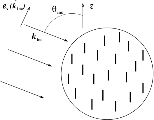
Figure 1: Uniformly anisotropic droplet. The polarisation vector $\mathbf{e}_{y}(\mathbf{\hat{k}}_{inc})$ is normal to the plane of the picture, $\mathbf{e}_{y}(\mathbf{\hat{k}}_{inc})\propto\mathbf{\hat{k}}_{inc}\times\mathbf{\hat{z}}$. Inside the droplet plane waves linearly polarised along $\mathbf{e}_{y}(\mathbf{\hat{k}}_{inc})$ represent ordinary waves.

The angle of incidence $\theta_{\rm inc}$ is the angle between the direction of incidence $\hat{k}$ and the direction of the uniform anisotropy. The $y$ direction is perpendicular to the plane made from these two directions. We shall show explicitly that the scattering process does not involve the $y$-component, $E_{y}^{(inc)}$, of the incoming plane wave

$$\mathbf{E}_{inc}=\mathbf{E}^{(inc)}\exp(i\,\mathbf{k}_{inc}\cdot\mathbf{r})\,,\quad\mathbf{E}^{(inc)}=E_{x}^{(inc)}\mathbf{e}_{x}(\mathbf{\hat{k}}_{inc})+E_{y}^{(inc)}\mathbf{e}_{y}(\mathbf{\hat{k}}_{inc})\,,\qquad\mathbf{k}_{inc}=k\mathbf{\hat{k}}_{inc}\,,$$ (1)

provided the refractive indices $n\equiv\sqrt{\epsilon}$ and $n_{o}\equiv\sqrt{\epsilon_{\perp}}$ are matched. In this paper we put the magnetic permittivity equal to the unit and slightly change the notations: $n_{0}$ and $\epsilon_{\perp}$ instead of $n_{1}$ and $\epsilon_{1}$. This corresponds to the physical condition in which there is a matching condition for the refracted ordinary wave inside the scattering droplet.

II.2 Equations for T-matrix

Since the electromagnetic field must be regular at the origin, the harmonics inside the droplet are now given by

$$\mathbf{E}_{jm}=\alpha_{jm}^{(c)}\,\mathbf{P}^{(m)}_{jm}(\rho_{o},\mathbf{\hat{r}})-n_{o}^{-1}\,\tilde{\alpha}_{jm}^{(c)}\,\mathbf{P}^{(e)}_{jm}(\rho_{o},\mathbf{\hat{r}})\,,$$ (2a)

$$\mathbf{H}_{jm}=\tilde{\alpha}_{jm}^{(c)}\,\mathbf{Q}^{(m)}_{jm}(\rho_{o},\mathbf{\hat{r}})+n_{o}\,\alpha_{jm}^{(c)}\,\mathbf{Q}^{(e)}_{jm}(\rho_{o},\mathbf{\hat{r}})\,,$$ (2b)

where $\rho_{o}=m_{o}kr=m_{o}\rho$ and $m_{o}\equiv n_{o}/n$ is the optical contrast. The modes $\mathbf{P}^{(\alpha)}_{jm}$ and $\mathbf{Q}^{(\alpha)}_{jm}$ have been given by Eqs. (27.I) for radial anisotropy and by Eqs. (43.I) for uniform anisotropy.

Following Eqs. (32.I), the continuity conditions at the outside of the droplet, $r=R_{1}$, can then be written in matrix notation as follows:

$$\sum_{j^{\prime}\geq|m|}\mathbf{R}_{1}^{jj^{\prime};\,m}\begin{pmatrix}\alpha_{j^{\prime}m}^{(c)}\\ \tilde{\alpha}_{j^{\prime}m}^{(c)}\end{pmatrix}=\boldsymbol{\Gamma}_{1}^{\,j}\begin{pmatrix}\alpha_{jm}^{(inc)}\\ \tilde{\alpha}_{jm}^{(inc)}\end{pmatrix}+\tilde{\boldsymbol{\Gamma}}_{1}^{\,j}\begin{pmatrix}\beta_{jm}^{(sca)}\\ \tilde{\beta}_{jm}^{(sca)}\end{pmatrix}\,,$$ (3)

$$\boldsymbol{\Gamma}^{\,j}(r)=\begin{pmatrix}j_{j}(\rho)&0\\ n[j_{j}(\rho)]^{\prime}&0\\ 0&j_{j}(\rho)\\ 0&-n^{-1}[j_{j}(\rho)]^{\prime}\end{pmatrix}\,,\quad\tilde{\boldsymbol{\Gamma}}^{\,j}(r)=\begin{pmatrix}h_{j}^{(1)}(\rho)&0\\ n[h_{j}^{(1)}(\rho)]^{\prime}&0\\ 0&h_{j}^{(1)}(\rho)\\ 0&-n^{-1}[h_{j}^{(1)}(\rho)]^{\prime}\end{pmatrix}\,,$$ (4)

where the index 1 indicates that matrix elements are calculated at the boundary of droplet, $r=R_{1}$.

In the case of a radially anisotropic droplet the matrix on the left hand side of Eq. (3) is diagonal over angular momentum numbers

$$\mathbf{R}^{jj^{\prime};\,m}(r)=\delta_{jj^{\prime}}\begin{pmatrix}j_{j}(\rho_{o})&0\\ n_{o}[j_{j}(\rho_{o})]^{\prime}&0\\ 0&j_{\tilde{j}}(\rho_{o})\\ 0&-n_{o}^{-1}[j_{\tilde{j}}(\rho_{o})]^{\prime}\end{pmatrix}\,,\quad\tilde{j}(\tilde{j}+1)=j(j+1)/(1+u)\,.$$ (5)

When the droplet is uniformly anisotropic, the matrix $\mathbf{R}^{jj^{\prime};\,m}(r)$ is no longer diagonal over angular momentum quantum numbers. In this case it takes the form:

$$\mathbf{R}^{jj^{\prime};\,m}(r)=\begin{pmatrix}p_{jj^{\prime};\,m}^{\,(m,m)}(\rho_{o})&-n_{o}^{-1}\,p_{jj^{\prime};\,m}^{\,(m,e)}(\rho_{o})\\ n_{o}\,q_{jj^{\prime};\,m}^{\,(e,e)}(\rho_{o})&q_{jj^{\prime};\,m}^{\,(e,m)}(\rho_{o})\\ n_{o}\,q_{jj^{\prime};\,m}^{\,(m,e)}(\rho_{o})&q_{jj^{\prime};\,m}^{\,(m,m)}(\rho_{o})\\ p_{jj^{\prime};\,m}^{\,(e,m)}(\rho_{o})&-n_{o}^{-1}\,p_{jj^{\prime};\,m}^{\,(e,e)}(\rho_{o})\end{pmatrix}\,,$$ (6)

where the coefficient functions are given by Eqs. (C3.I)-(C10.I) in Appendix C of I.

The system (3) can be then simplified by multiplying both sides by the matrices

$$\mathbf{H}^{\,j}(r)=-i\,\rho^{2}\,\begin{pmatrix}[j_{j}(\rho)]^{\prime}&-n^{-1}\,j_{j}(\rho)&0&0\\ 0&0&n^{-1}\,[j_{j}(\rho)]^{\prime}&j_{j}(\rho)\end{pmatrix}\,,$$ (7a)

$$\tilde{\mathbf{H}}^{\,j}(r)=-i\,\rho^{2}\,\begin{pmatrix}[h_{j}^{(1)}(\rho)]^{\prime}&-n^{-1}\,h_{j}^{(1)}(\rho)&0&0\\ 0&0&n^{-1}\,[h_{j}^{(1)}(\rho)]^{\prime}&h_{j}^{(1)}(\rho)\end{pmatrix}\,.$$ (7b)

Using the fact that the Wronskian for spherical Bessel functions is given by Abramowitz and Stegun (1972):

$$W\{j_{j}(\rho),h_{j}^{(1)}(\rho)\}=i/\rho^{2}\,,$$

we derive a system equivalent to Eqs. (3) in the following form:

$$\begin{pmatrix}\alpha_{jm}^{(inc)}\\ n^{-1}\,\tilde{\alpha}_{jm}^{(inc)}\end{pmatrix}=\sum_{j^{\prime}\geq|m|}\mathbf{B}_{jj^{\prime};\,m}\begin{pmatrix}\alpha_{j^{\prime}m}^{(c)}\\ \tilde{\alpha}_{j^{\prime}m}^{(c)}\end{pmatrix}\,,$$ (8a)

$$\begin{pmatrix}\beta_{jm}^{(sca)}\\ n^{-1}\,\tilde{\beta}_{jm}^{(sca)}\end{pmatrix}=\sum_{j^{\prime}\geq|m|}\mathbf{A}_{jj^{\prime};\,m}\begin{pmatrix}\alpha_{j^{\prime}m}^{(c)}\\ \tilde{\alpha}_{j^{\prime}m}^{(c)}\end{pmatrix}\,,$$ (8b)

where $\mathbf{A}_{jj^{\prime};\,m}=-\mathbf{H}_{1}^{\,j}\cdot\mathbf{R}_{1}^{jj^{\prime};\,m}$ and $\mathbf{B}_{jj^{\prime};\,m}=\tilde{\mathbf{H}}_{1}^{\,j}\cdot\mathbf{R}_{1}^{jj^{\prime};\,m}$.

These are the equivalent of the equations (51.I) for scattering by a spherical annulus. The equations are considerably simpler, as a result of what might be called mode decoupling. The crucial point is that the normal modes inside the droplet are all regular at the origin, and thus two types of modes which appear in the case of the annulus do not appear here. This reduces the number of variables in the problem by one half, even in the case of the uniform anisotropy which, at least in principle, presented a certain number of problems in the annular case.

From Eq. (8) we can immediately derive an expression for the T-matrix:

$$\mathbf{T}_{jj^{\prime};\,m}=[\mathbf{A}\cdot\mathbf{B}^{-1}]_{jj^{\prime};\,m}\,.$$ (9)

For radial anisotropy all the matrices on the right hand sides of Eqs. (8) are diagonal. So, it is easy to write down the result for the T-matrix:

$$\mathbf{T}_{jj^{\prime};\,m}=\delta_{jj^{\prime}}\begin{pmatrix}T_{j}^{11}&0\\ 0&T_{j}^{22}\end{pmatrix}\,,$$ (10)

where

$$T_{j}^{11}=-\frac{[j_{j}(\rho_{o})]_{1}\,[j_{j}(\rho)]^{\prime}_{1}-m_{o}\,[j_{j}(\rho_{o})]^{\prime}_{1}\,[j_{j}(\rho)]_{1}}{[j_{j}(\rho_{o})]_{1}\,[h_{j}^{(1)}(\rho)]^{\prime}_{1}-m_{o}\,[j_{j}(\rho_{o})]^{\prime}_{1}\,[h_{j}^{(1)}(\rho)]_{1}}\,,$$ (11a)

$$T_{j}^{22}=-\frac{m_{o}\,[j_{\tilde{j}}(\rho_{o})]_{1}\,[j_{j}(\rho)]^{\prime}_{1}-[j_{\tilde{j}}(\rho_{o})]^{\prime}_{1}\,[j_{j}(\rho)]_{1}}{m_{o}\,[j_{\tilde{j}}(\rho_{o})]_{1}\,[h_{j}^{(1)}(\rho)]^{\prime}_{1}-[j_{\tilde{j}}(\rho_{o})]^{\prime}_{1}\,[h_{j}^{(1)}(\rho)]_{1}}\,.$$ (11b)

These formulae bear close resemblance to the well known Mie expressions Boren and Huffman (1983).

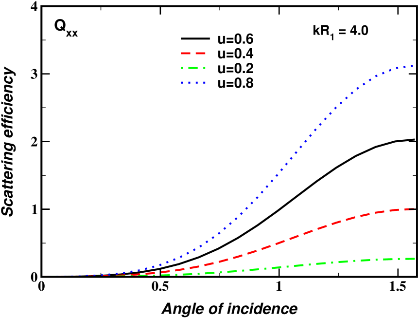
Figure 2: Scattering efficiency of uniformly anisotropic droplet as a function the angle of incidence (the angle between the incident wave and the optical axis) at various values of the anisotropy parameter, $u=(\epsilon_{\parallel}-\epsilon_{\perp})/\epsilon_{\perp}$, with $kR_{1}=4.0$ and $n=n_{o}$.

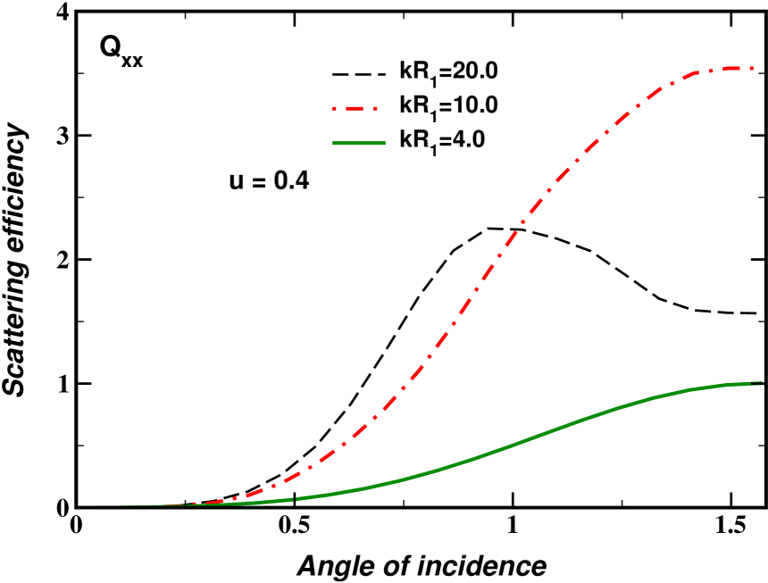
Figure 3: Dependence of the scattering efficiency on the angle of incidence for uniformly anisotropic droplet at various values of the size parameter and $u=0.4$. The refractive indices $n$ and $n_{o}$ are matched.

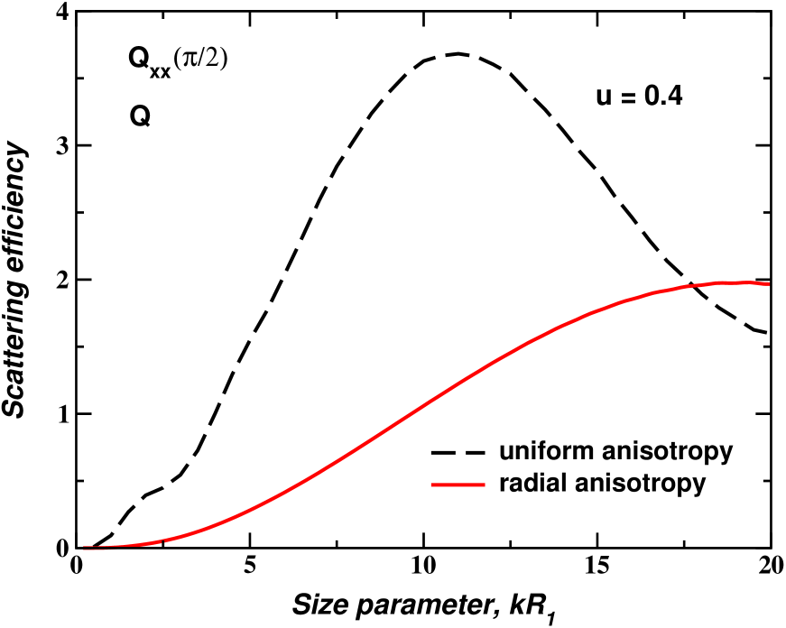
Figure 4: Scattering efficiencies of radially and uniformly anisotropic droplets versus the size parameter at $u=0.4$, $\theta_{inc}=\pi/2$ and $n=n_{o}$.

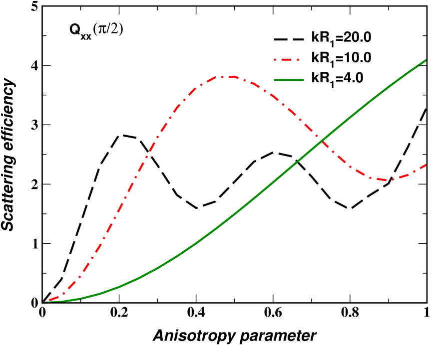
Figure 5: Scattering efficiencies of radially and uniformly anisotropic droplets versus the anisotropy parameter at various values of the size parameter for $\theta_{inc}=\pi/2$ and $n=n_{o}$.

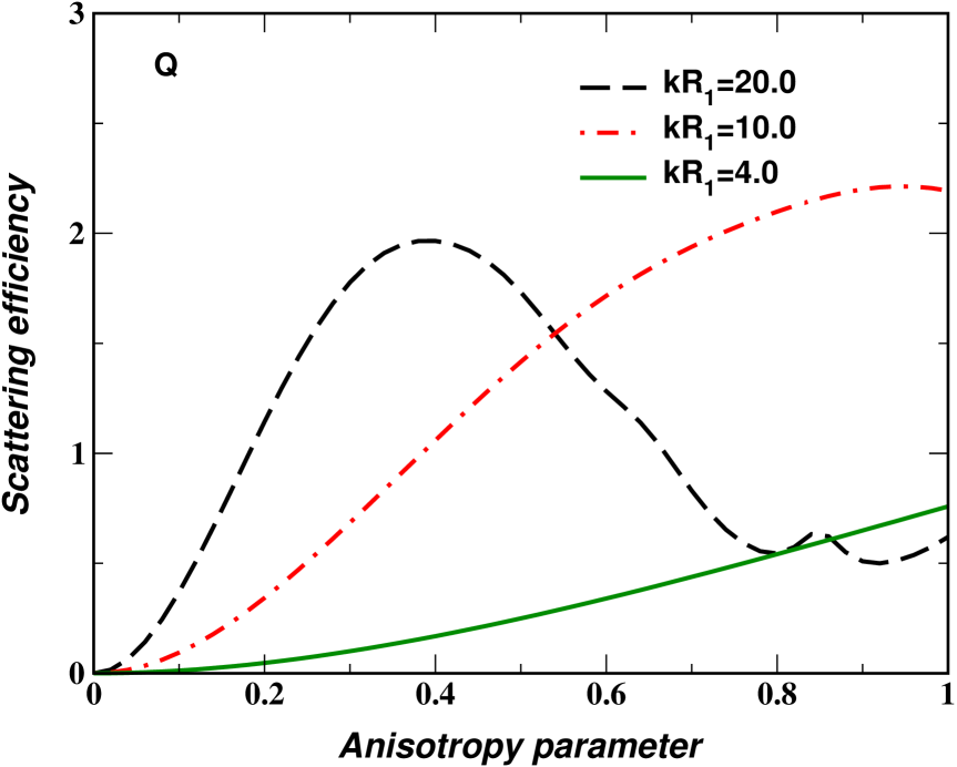
Figure 6: Dependence of the scattering efficiency on the anisotropy parameter for radially anisotropic droplet at various values of the size parameter and $n=n_{o}$.

II.3 Scattering efficiency

We have seen in I that the total scattering cross-section for the uniformly anisotropic scatterer depends on the angle of incidence $\theta_{inc}$. The scattering cross-section also depends on the polarisation of the incident wave. In order to emphasise this, let us express the coefficients of the incident wave $\alpha_{jm}^{(inc)}$ and $\tilde{\alpha}_{jm}^{(inc)}$ (see Eq. (9.I)) as follows

$$\alpha_{jm}^{(inc)}=\alpha_{jm;\,x}^{(inc)}\,E_{x}^{(inc)}+\alpha_{jm;\,y}^{(inc)}\,E_{y}^{(inc)}\,,$$ (12a)

$$\tilde{\alpha}_{jm}^{(inc)}=\tilde{\alpha}_{jm;\,x}^{(inc)}\,E_{x}^{(inc)}+\tilde{\alpha}_{jm;\,y}^{(inc)}\,E_{y}^{(inc)}\,,$$ (12b)

where

$$\alpha_{jm;\,x}^{(inc)}=i^{j}\,[\pi(2j+1)]^{1/2}D_{jm}^{(y)}(\mathbf{\hat{k}}_{inc})\,,\quad\alpha_{jm;\,y}^{(inc)}=i^{j+1}\,[\pi(2j+1)]^{1/2}D_{jm}^{(x)}(\mathbf{\hat{k}}_{inc})\,,$$

$$\tilde{\alpha}_{jm;\,x}^{(inc)}=n\,i^{j+1}\,[\pi(2j+1)]^{1/2}D_{jm}^{(x)}(\mathbf{\hat{k}}_{inc})\,,\quad\tilde{\alpha}_{jm;\,y}^{(inc)}=-n\,i^{j}\,[\pi(2j+1)]^{1/2}D_{jm}^{(y)}(\mathbf{\hat{k}}_{inc})\,.$$ (13)

From Eq. (19.I) the scattering efficiency then can be rewritten in the following form:

$$Q=\frac{S_{sca}}{\pi R_{1}^{2}}=I_{inc}^{-1}\sum_{\alpha=x,y}\sum_{\beta=x,y}Q_{\alpha\beta}E_{\alpha}^{(inc)}E_{\beta}^{(inc)\,*}\,,$$ (14)

$$Q_{\alpha\beta}=(kR_{1})^{-2}\pi^{-1}\sum_{jm}\left[\beta_{jm;\,\alpha}^{(sca)}\beta_{jm;\,\beta}^{(sca)\,*}+n^{-2}\tilde{\beta}_{jm;\,\alpha}^{(sca)}\tilde{\beta}_{jm;\,\beta}^{(sca)\,*}\right]\,,$$ (15)

$$\begin{pmatrix}\beta_{jm;\,\alpha}^{(sca)}\\ n^{-1}\,\tilde{\beta}_{jm:\,\alpha}^{(sca)}\end{pmatrix}=\sum_{j^{\prime}}\mathbf{T}_{jj^{\prime};\,m}\begin{pmatrix}\alpha_{j^{\prime}m;\,\alpha}^{(inc)}\\ n^{-1}\,\tilde{\alpha}_{j^{\prime}m;\,\alpha}^{(inc)}\end{pmatrix}\,.$$ (16)

Note that for radial anisotropy $Q_{\alpha\beta}=\delta_{\alpha\beta}\,Q$. By contrast, in the case of uniformly anisotropic droplet we have rather strong dependence of the scattering efficiency on the polarisation of the incoming wave. When the refractive indices are matched, $n=n_{o}$, it is expected that the scatterer does not change the $y$ component of the incident wave, which simply transforms into the ordinary wave inside the droplet without being affected by the scattering process. The algebraic interpretation of this fact is that the amplitudes of the scattered wave $\beta_{jm;\,y}^{(sca)}$ and $\tilde{\beta}_{jm;\,y}^{(sca)}$ are equal to zero. However, it is not straightforward to see that the system (8) is consistent with this conclusion. We show this in Appendix A; the proof involves using relations (46.I) in which the electric and magnetic fields inside the droplet are expressed in terms of appropriate normal modes.

III Numerical results

In this section we present numerical results for the scattering efficiency defined by Eqs. (14) and (15). We are primarily interested in anisotropy-induced scattering. In order to concentrate on this test case, we consider the case when the refractive indices $n$ and $n_{o}$ are equal. We shall present a more comprehensive analysis of all possible cases, including the results for the angular distribution of the scattered waves, elsewhere. We begin with brief comments on numerical procedure and then proceed with the description of the calculated dependencies.

It is rather straightforward to perform computations for radially anisotropic droplets. The expressions for the elements of T-matrix are known and given by Eqs. (11a)-(11b). We can thus evaluate the scattering efficiency by explicitly computing the sum in the expression (22.I).

For uniformly anisotropic droplets T-matrix can only be computed numerically by solving the system of equations (8) . Some highlights of the results are presented below.

The dependence of the scattering efficiency on the angle of incidence is shown in Fig. 2. If the size parameter, $kR_{1}$, is not very large, the scattering efficiency $Q_{xx}$ is a monotonically increasing function of the angle of incidence, $\theta_{inc}$, in the region from 0 to $\pi/2$. By symmetry $Q_{xx}(\theta_{inc})=Q_{xx}(\pi/2-\theta_{inc})$, and so the scattering efficiency decreases in the range from $\pi/2$ to $\pi$.

In Fig. 3 we show what happens for shorter wavelength and thus higher values of $kR_{1}$. Now, for for relatively large values of the size parameter, the cross-section dependence on the angle is incidence is no longer monotonic. For example, at $kR_{1}=20.0$, the angle at which the scattering efficiency $Q_{xx}$ reaches its maximum value is no longer at $\pi/2$.

Fig. 4 shows the scattering efficiencies $Q_{xx}(\pi/2)$ (for uniform anisotropy) and $Q$ (for radial anisotropy) versus the size parameter. The scattering efficiency of uniformly anisotropic droplet has a pronounced peak located at about $kR_{1}\approx 10.0$ and exhibits strongly non-monotonic behaviour. By contrast, the corresponding dependence for the radially anisotropic droplet is monotonically increasing. In this case the first maximum is reached at $kR_{1}\approx 20.0$, outside the range of $kR_{1}$ shown in Fig. 4.

The scattering efficiencies as a function of the anisotropy parameter, $0\leq u\leq 1$, at different values of the size parameter are plotted in Fig. 5 and Fig. 6 for the cases of radial and uniform anisotropies respectively. In both cases an increase in the size parameter leads to the appearance of peaks in this range of $u$. As compared to radially anisotropic scatterers, the uniformly anisotropic droplets seem to be more sensitive to changes both in the size and in the anisotropy parameters .

IV Conclusion

In this work we have described some of the numerical results calculated using the T-matrix theory developed in paper I. In particular, we have studied the scattering efficiency of radially and uniformly anisotropic droplets in which the ordinary refractive index matches the refractive index of the material surrounding them.

The assumption in which the ordinary refractive index of the droplet matches the isotropic dielectric constant in the surrounding medium is not taken in order to simplify the numerical treatment. Rather in this paper we wish to study the light scattering properties which can be solely attributed to the anisotropic part of the dielectric tensor. Thus we have the anisotropy effects separated out to concentrate on differences between isotropic and anisotropic optical axis distributions.

Clearly, the difference in symmetry causes the most crucial differences in the light scattering. For uniformly anisotropic droplets the scattering efficiency depends on the angle of incidence and the polarisation of incoming wave, whereas for radially anisotropic scatterers it does not. In other words, the scattering from radially anisotropic droplet shares some features of isotropic scatterers.

Nevertheless, the angular dependencies for the scattered wave intensity and the depolarisation factor shown at the end of I clearly indicate the pronounced differences.

The graphs plotted in Figs. 4-6 indicate that uniformly anisotropic droplets are more sensitive to changes in the wavelength and anisotropy parameters than are radially anisotropic droplets. Our results are also consistent with results of previous studies Žumer (1988); Kiselev et al. (2000) that the internal spatial distribution of the optical axis is a factor which strongly affects light scattering from anisotropic scatterers.

The results of this work can be regarded as the first step towards more comprehensive study of light scattering by anisotropic scatterers. We have demonstrated that the T-matrix approach developed in I can be used in an efficient numerical treatment of the scattering problem. It is thus reasonable to expect that further progress can be made by applying this theory to more complex problems involving light scattering by optical anisotropic liquid crystalline systems and other related problems, as discussed further in the last section of I.

Appendix A

In this appendix we show mathematically, suing our formalism, the physically obvious result that if the ordinary refractive index of a droplet matches that of the scattering medium, then there will be no scattering of the polarisation component out of the plane of the incident wave and the uniform anisotropy in the droplet. In order to do this, we first extend algebraic relations that follow from Eqs. (46.I). These equations give the expansion of plane wave propagating in a uniformly anisotropic medium. We can rewrite them for the plane wave inside the droplet:

$$\sum_{j^{\prime}m^{\prime}}\left[\,\alpha_{j^{\prime}m^{\prime}}^{(inc)}\,\mathbf{P}^{(m)}_{j^{\prime}m^{\prime}}(\rho_{o},\mathbf{\hat{r}})-n_{o}^{-1}\,\tilde{\alpha}_{j^{\prime}m^{\prime}}^{(inc)}\,\mathbf{P}^{(e)}_{j^{\prime}m^{\prime}}(\rho_{o},\mathbf{\hat{r}})\,\right]=$$

$$=\exp(i\rho_{e}\,\mathbf{\hat{k}}_{inc}\cdot\mathbf{\hat{r}})E_{x}(\mathbf{\hat{k}}_{inc})\bigl{[}\mathbf{e}_{x}(\mathbf{\hat{k}}_{inc})+\frac{u}{1+u}\,\sin\theta_{inc}\,\mathbf{\hat{z}}\bigr{]}+\exp(i\rho_{o}\,\mathbf{\hat{k}}_{inc}\cdot\mathbf{\hat{r}})E_{y}(\mathbf{\hat{k}}_{inc})\,\mathbf{e}_{y}(\mathbf{\hat{k}}_{inc})\,,$$ (17)

$$\sum_{j^{\prime}m^{\prime}}\left[\,\tilde{\alpha}_{j^{\prime}m^{\prime}}^{(inc)}\,\mathbf{Q}^{(m)}_{j^{\prime}m^{\prime}}(\rho_{o},\mathbf{\hat{r}})+n_{o}\,\alpha_{j^{\prime}m^{\prime}}^{(inc)}\,\mathbf{Q}^{(e)}_{j^{\prime}m^{\prime}}(\rho_{o},\mathbf{\hat{r}})\,\right]=$$

$$=n_{o}\left(\,\exp(i\rho_{e}\mathbf{\hat{k}}_{inc}\cdot\mathbf{\hat{r}})\,m_{e}^{-1}\,E_{x}(\mathbf{\hat{k}}_{inc})\mathbf{e}_{y}(\mathbf{\hat{k}}_{inc})-\exp(i\rho_{o}\,\mathbf{\hat{k}}_{inc}\cdot\mathbf{\hat{r}})E_{y}(\mathbf{\hat{k}}_{inc})\mathbf{e}_{x}(\mathbf{\hat{k}}_{inc})\,\right)\,,$$ (18)

where $\rho_{e}=m_{e}\rho_{o}$ and $m_{e}=\sqrt{(1+u)/(1+u\cos^{2}\theta_{inc})}$. The coefficients $\alpha_{jm}^{(inc)}$ and $\tilde{\alpha}_{jm}^{(inc)}$ are defined by Eqs. (9.I) where the factor $\mu/n$ is changed to $1/n_{o}$.

We can now combine the relations that come from definitions of the coefficient functions (see Eq. (45.I))

$$\sum_{j^{\prime}\geq|m|}\left[p_{jj^{\prime};\,m}^{\,(\alpha,m)}(\rho_{o})\,\alpha_{j^{\prime}m}^{(inc)}-n_{o}^{-1}p_{jj^{\prime};\,m}^{\,(\alpha,e)}(\rho_{o})\,\tilde{\alpha}_{j^{\prime}m}^{(inc)}\right]=$$

$$=\Bigl{\langle}\,\mathbf{Y}_{jm}^{(\alpha)\,*}(\mathbf{\hat{r}})\cdot\sum_{j^{\prime}m^{\prime}}\left[\,\alpha_{j^{\prime}m^{\prime}}^{(inc)}\,\mathbf{P}^{(m)}_{j^{\prime}m^{\prime}}(\rho_{o},\mathbf{\hat{r}})-n_{o}^{-1}\,\tilde{\alpha}_{j^{\prime}m^{\prime}}^{(inc)}\,\mathbf{P}^{(e)}_{j^{\prime}m^{\prime}}(\rho_{o},\mathbf{\hat{r}})\,\right]\,\Bigr{\rangle}_{\mathbf{\hat{r}}}\,,$$ (19)

$$\sum_{j^{\prime}\geq|m|}\left[n_{o}\,q_{jj^{\prime};\,m}^{\,(\alpha,e)}(\rho_{o})\,\alpha_{j^{\prime}m}^{(inc)}+q_{jj^{\prime};\,m}^{\,(\alpha,m)}(\rho_{o})\,\tilde{\alpha}_{j^{\prime}m}^{(inc)}\right]=$$

$$=\Bigl{\langle}\,\mathbf{Y}_{jm}^{(\alpha)\,*}(\mathbf{\hat{r}})\cdot\sum_{j^{\prime}m^{\prime}}\left[\,\tilde{\alpha}_{j^{\prime}m^{\prime}}^{(inc)}\,\mathbf{Q}^{(m)}_{j^{\prime}m^{\prime}}(\rho_{o},\mathbf{\hat{r}})+n_{o}\,\alpha_{j^{\prime}m^{\prime}}^{(inc)}\,\mathbf{Q}^{(e)}_{j^{\prime}m^{\prime}}(\rho_{o},\mathbf{\hat{r}})\,\right]\,\Bigr{\rangle}_{\mathbf{\hat{r}}}\,,\;\alpha\in\{m,e\}\,,$$ (20)

with the relations (17)-(18) to evaluate the left hand side of the system (3) provided that $\{\alpha_{jm}^{(c)},\tilde{\alpha}_{jm}^{(c)}\}=\{\alpha_{jm}^{(inc)},\tilde{\alpha}_{jm}^{(inc)}\}$.

To this end, we can use Eq. (6) to write down the sum on the left hand side of Eq. (3) in the following form:

$$\sum_{j^{\prime}\geq|m|}\mathbf{R}^{jj^{\prime};\,m}(r)\begin{pmatrix}\alpha_{j^{\prime}m}^{(inc)}\\ \tilde{\alpha}_{j^{\prime}m}^{(inc)}\end{pmatrix}=\sum_{j^{\prime}\geq|m|}\begin{pmatrix}p_{jj^{\prime};\,m}^{\,(m,m)}(\rho_{o})\,\alpha_{j^{\prime}m}^{(inc)}-n_{o}^{-1}p_{jj^{\prime};\,m}^{\,(m,e)}(\rho_{o})\,\tilde{\alpha}_{j^{\prime}m}^{(inc)}\\ n_{o}\,q_{jj^{\prime};\,m}^{\,(e,e)}(\rho_{o})\,\alpha_{j^{\prime}m}^{(inc)}+q_{jj^{\prime};\,m}^{\,(e,m)}(\rho_{o})\,\tilde{\alpha}_{j^{\prime}m}^{(inc)}\\ n_{o}\,q_{jj^{\prime};\,m}^{\,(m,e)}(\rho_{o})\,\alpha_{j^{\prime}m}^{(inc)}+q_{jj^{\prime};\,m}^{\,(m,m)}(\rho_{o})\,\tilde{\alpha}_{j^{\prime}m}^{(inc)}\\ p_{jj^{\prime};\,m}^{\,(e,m)}(\rho_{o})\,\alpha_{j^{\prime}m}^{(inc)}-n_{o}^{-1}p_{jj^{\prime};\,m}^{\,(e,e)}(\rho_{o})\,\tilde{\alpha}_{j^{\prime}m}^{(inc)}\end{pmatrix}\,.$$ (21)

It is seen that the elements of the column on the right hand side of this equation are the sums from the left hand sides of Eqs. (19) and (20). On the other hand, from Eqs. (17)-(18), the square bracketed sums on the right hand sides of Eqs. (19)-(20) are the plane waves. So, the elements of the column (21) can be evaluated as scalar products of the vector spherical functions and the vector plane waves by using Eqs. (B6.I) and (B8.I) of appendix B in I.

We can now apply this procedure to calculate the elements of the column (21) for the ordinary wave with $\{\alpha_{jm}^{(inc)},\tilde{\alpha}_{jm}^{(inc)}\}=\{\alpha_{jm;\,y}^{(inc)},\tilde{\alpha}_{jm;\,y}^{(inc)}\}$. From Eqs. (12a)-(12b) we have $E_{x}(\mathbf{\hat{k}}_{inc})=0$ and $E_{y}(\mathbf{\hat{k}}_{inc})=1$ in this case. The final result is

$$\sum_{j^{\prime}\geq|m|}\mathbf{R}^{jj^{\prime};\,m}(r)\begin{pmatrix}\alpha_{j^{\prime}m;\,y}^{(inc)}\\ \tilde{\alpha}_{j^{\prime}m;\,y}^{(inc)}\end{pmatrix}=\alpha_{jm;\,y}^{(inc)}\begin{pmatrix}j_{j}(\rho_{o})\\ n_{o}\,[j_{j}(\rho_{o})]^{\prime}\\ 0\\ 0\end{pmatrix}+n_{o}^{-1}\,\tilde{\alpha}_{jm;\,y}^{(inc)}\begin{pmatrix}0\\ 0\\ n_{o}\,j_{j}(\rho_{o})\\ -[j_{j}(\rho_{o})]^{\prime}\end{pmatrix}\,.$$ (22)

When $n_{o}=n$ (and $\rho=\rho_{o}$), after multiplying (22) by the matrices (7), we have

$$\sum_{j^{\prime}\geq|m|}\mathbf{B}_{jj^{\prime};\,m}\begin{pmatrix}\alpha_{j^{\prime}m;\,y}^{(inc)}\\ \tilde{\alpha}_{j^{\prime}m;\,y}^{(inc)}\end{pmatrix}=\begin{pmatrix}\alpha_{jm;\,y}^{(inc)}\\ n^{-1}\,\tilde{\alpha}_{jm;\,y}^{(inc)}\end{pmatrix}\,,\quad\sum_{j^{\prime}\geq|m|}\mathbf{A}_{jj^{\prime};\,m}\begin{pmatrix}\alpha_{j^{\prime}m;\,y}^{(inc)}\\ \tilde{\alpha}_{j^{\prime}m;\,y}^{(inc)}\end{pmatrix}=\begin{pmatrix}0\\ 0\end{pmatrix}\,.$$ (23)

From these equations we immediately conclude that, when $n=n_{o}$ and $\{\alpha_{jm}^{(inc)},\tilde{\alpha}_{jm}^{(inc)}\}=\{\alpha_{jm;\,y}^{(inc)},\tilde{\alpha}_{jm;\,y}^{(inc)}\}$, the solution of the system (8) is given by

$$\alpha_{jm}^{(c)}=\alpha_{jm;\,y}^{(inc)},\quad\tilde{\alpha}_{jm}^{(c)}=\tilde{\alpha}_{jm;\,y}^{(inc)},\quad\beta_{jm}^{(sca)}\equiv\beta_{jm;\,y}^{(sca)}=0,\quad\tilde{\beta}_{jm}^{(sca)}\equiv\tilde{\beta}_{jm;\,y}^{(sca)}=0\,.$$ (24)

So, the amplitudes of scattered wave $\beta_{jm;\,y}^{(sca)}$ and $\tilde{\beta}_{jm;\,y}^{(sca)}$ vanish at $n=n_{o}$.

References

• Kiselev et al. (2001) A. Kiselev, V. Reshetnyak, and T. Sluckin, Light scattering by optically anisotropic scatterers I: T-matrix theory for radial and uniform anisotropies (2001), [paper I, preceding paper].
• Newton (1982) R. Newton, Scattering Theory of Waves and Particles (Springer, Heidelberg, 1982), 2nd ed.
• Žumer and Doane (1986) S. Žumer and J. Doane, Phys. Rev. A 34, 3373 (1986).
• Žumer (1988) S. Žumer, Phys. Rev. A 37, 4006 (1988).
• Mishchenko et al. (2000) M. Mishchenko, J. Hovenier, and L. Travis, eds., Light Scattering by Nonspherical Particles: Theory, Measurements and Applications (Academic Press, New York, 2000).
• Roth and Digman (1973) J. Roth and M. Digman, J. Opt. Soc. Am. 63, 308 (1973).
• Kiselev et al. (2000) A. Kiselev, V. Reshetnyak, and T. Sluckin, Opt. Spectrosc. 89(6), 907 (2000).
• Boren and Huffman (1983) C. Boren and D. Huffman, Absorption and Scattering of Light by Small Particles (Wiley-Interscience, New York, 1983).
• Abramowitz and Stegun (1972) M. Abramowitz and I. Stegun, eds., Handbook of Mathematical Functions (Dover, New York, 1972).