Light scattering by optically anisotropic scatterers I:
T–matrix theory for radial and uniform anisotropies

Abstract

We extend the T-matrix approach to light scattering by spherical particles to some simple cases in which the scatterers are optically anisotropic. Specifically we consider cases in which the spherical particles include radially and uniformly anisotropic layers. We find that in both cases the T-matrix theory can be formulated using a modified T-matrix ansatz with suitably defined modes. In a uniformly anisotropic medium we derive these modes by relating the wave packet representation and expansions of electromagnetic field over spherical harmonics. The resulting wave functions are deformed spherical harmonics that represent solutions of the Maxwell equations. We use these modes to express the equations for the T-matrix elements in terms of computationally tractable coefficient functions.

I Introduction

The problem of light scattering by particles of one medium embedded in another has a long history, dating back almost a century to the classical exact solution due to Mie Mie (1908). The Mie solution applies to scattering by uniform spherical particles with isotropic dielectric properties. More recently this strategy has been successfully applied to ellipsoidal particles and some circumstances in which the dielectric tensor is anisotropic  Asano and Yamamoto (1975); Roth and Digman (1973); Lange and Aragon (1990); Hahn and Aragon (1994); Karacali et al. (1997); Kiselev et al. (2000a, b).

Unfortunately, Mie–type solutions, although exact, are not always physically meaningful. An alternative strategy useful in the long wavelength limit is the so-called Rayleigh-Gans (R-G) approximation Newton (1982), which is closely allied to the classic Born approximation of quantum mechanics. However, detailed information on the precise range of validity of this approximation often requires solution of the Mie problem, which is only available in some specific cases.

There are a large number of physical contexts in which it is useful to understand light scattering by impurities Ishimaru (1978). A particular example of recent interest concerns liquid crystal devices. There are now a number of systems in which liquid crystal droplets are suspended in a polymer matrix – the so-called PDLC systems – or the inverse system, involving colloids now with a nematic liquid crystal solvent. These inverse systems are commonly known as filled nematics Kreuzer and Eidenschink (1996); Bellini et al. (1998).

In such systems one needs to calculate light scattering by composite anisotropic particles embedded in an isotropic or an anisotropic matrix. The model scatterer usually consists of a small central isotropic particle (“the core”), coated by a much larger region in which the optical tensor is anisotropic. This is equivalent to examining light scattering by a composite particle consisting of the central core plus a surrounding liquid crystalline layer.

The analysis of a Mie–type theory uses a systematic expansion of the electromagnetic field over vector spherical harmonics. The specific form of the expansions is known as the T–matrix ansatz. This has been widely used in the related problem of light scattering by nonspherical particles Mishchenko et al. (1996, 2000).

Recently in Kiselev et al. (2000a, b) we have studied the scattering problem for the optical axis distributions of the form: $n_{r}\mathbf{\hat{r}}+n_{\vartheta}\boldsymbol{\hat{\vartheta}}+n_{\varphi}\boldsymbol{\hat{\varphi}}$. By using separation of variables and expansions over vector spherical harmonics, we have developed the generalised Mie theory as an extension of the T–matrix ansatz Mishchenko et al. (1996). This theory combines computational efficiency of the T–matrix approach and well defined transformation properties of the spherical harmonics under rotations.

In this paper we discuss this theory in more detail and explain how this approach can be extended to the case of uniformly anisotropic spherical particles.

The layout of the paper is as follows. General discussion of the model is given in Sec. II. Then in Sec. III we outline the T-matrix formalism for the isotropic medium in the form suitable for subsequent generalisation. In Sec. IV, as the simplest case to start from, we consider how the T–matrix ansatz applies for the radially anisotropic layer. We find that the structure of electromagnetic modes in the layer requires modification of the standard T-matrix ansatz. In addition, we detail computing the elements of T-matrix.

In Sec. V we describe the method to put the scattering problem into the language of T–matrix by linking the representations of plane wave packets and of spherical harmonics. For uniformly anisotropic scatterer we define generalised spherical harmonics and show that the effect of angular momentum mixing can be treated efficiently.

Finally in Sec. VI we draw together the results and make some concluding remarks. In particular, we emphasise the importance of anisotropy effects by making comparison between angular distributions of scattered wave intensities for radially anisotropic layer and effective isotropic layer of the same scattering efficiency.

Details on some technical results are relegated to Appendices A – C.

II Model

We consider scattering by a spherical particle of radius $R_{1}$ embedded in a uniform isotropic dielectric medium with dielectric constant $\epsilon_{ij}=\epsilon\delta_{ij}$ and magnetic permeability $\mu_{ij}=\mu\delta_{ij}$. The scattering particle consists of an inner isotropic core of radius $R_{2}$, surrounded by an anisotropic annular layer of thickness $d=R_{1}-R_{2}$.

Within the inner core of the scatterer the dielectric tensor $\boldsymbol{\epsilon}$, and the magnetic permittivity $\boldsymbol{\mu}$ take the values $\boldsymbol{\epsilon}_{ij}=\epsilon_{2}\delta_{ij}$, $\boldsymbol{\mu}_{ij}=\mu_{2}\delta_{ij}$. The dielectric tensor within the annular layer is locally uniaxial. The optical axis distribution is defined by the vector field $\mathbf{\hat{n}}$. (Hats will denote unit vectors.) Then within the annular layer $\boldsymbol{\epsilon}_{ij}({\bf r})=\epsilon_{1}\delta_{ij}+\Delta\epsilon_{1}(\mathbf{\hat{n}}({\bf r})\otimes\mathbf{\hat{n}}({\bf r}))_{ij}$ and $\boldsymbol{\mu}_{ij}=\mu_{1}\delta_{ij}$. The unit vector $\mathbf{\hat{n}}$ corresponds to a liquid crystal director for material within the annular region.

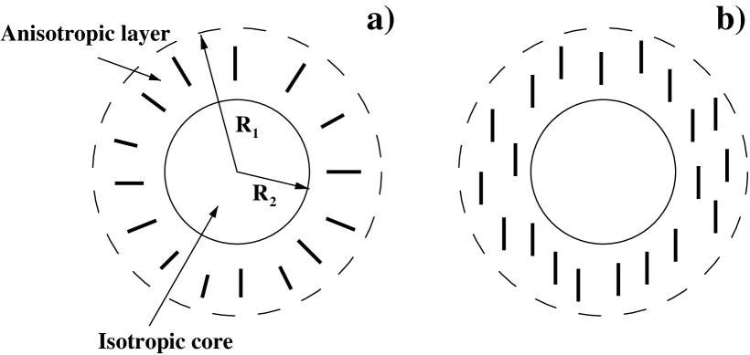
Figure 1: Distributions of optical axis in the anisotropic layer around a spherical particle for radial and uniform structures: a) $\mathbf{\hat{n}}=\mathbf{\hat{r}}$; b) $\mathbf{\hat{n}}=\mathbf{\hat{z}}$

We shall suppose that the director field can be written in one of the following forms

$$\mathbf{\hat{n}}=\mathbf{\hat{z}}$$ (1a)

$$\mathbf{\hat{n}}=\mathbf{\hat{r}}$$ (1b)

where $\mathbf{\hat{r}}=(\sin\theta\cos\phi,\sin\theta\sin\phi,\cos\theta)$ is the unit radial vector; $\phi$ and $\theta$ are Euler angles of the unit vector $\mathbf{\hat{r}}$. $\mathbf{\hat{x}}$, $\mathbf{\hat{y}}$ and $\mathbf{\hat{z}}$ are the unit vectors directed along the corresponding coordinate axes.

In Fig. 1 we have shown these director distributions. Fig. 1a shows the radial (and spherically symmetric) director distribution. The scattering problem in this case has already been discussed by Roth and Digman Roth and Digman (1973), and in this case the spherical symmetry of the problem plays an important role in rendering the Maxwell equations soluble.

We show in Fig. 1b the case in which the optical axis is directed along the $z$–axis and is uniformly distributed within the annular layer; this is given by Eq. (1a). The case where the scatterer is a long cylinder parallel to $\mathbf{\hat{n}}$ presents no difficulties and can be treated in cylindrical coordinate system Boren and Huffman (1983). Scattering from spherical uniformly anisotropic particles is not exactly soluble Boren and Huffman (1983) and has been studied by using the Rayleigh–Gans method and the anomalous diffraction approximation in Žumer and Doane (1986); Žumer (1988).

A simple limit of the physical situations we consider puts $\epsilon=\epsilon_{1}=\epsilon_{2}$, with $\mu=\mu_{1}=\mu_{2}$. The first condition allows us to concentrate on situations in which the scattering is governed by the anisotropic part of the dielectric properties. This distinguishes our case from other studies of scattering by spheres, in which the isotropic optical contrast dominates. However, there is also a motivation for this hypothesis in terms of liquid crystal device physics, and we shall discuss this at greater length in a subsequent paper. However, the result of the hypothesis is that the scattering by our model spheres disappears in the limit of zero anisotropy.

III T–matrix approach in isotropic medium

III.1 T–matrix ansatz

In this subsection we remind the reader about the relationship between Maxwell’s equations in the region of a scatterer and the formulation of scattering properties in terms of the T–matrix Newton (1982); Ishimaru (1978). Our formulation is slightly non-standard. Some technical details, which can be omitted at first reading, have been relegated to the appendices.

We shall need to write the Maxwell equations for a harmonic electromagnetic wave (time–dependent factor is $\exp\{-i\omega t\}$) in the form:

$$-in_{i}[\mu_{i}k_{i}]^{-1}\,\boldsymbol{\nabla}\times\mathbf{E} =\mathbf{H}\,,$$ (2a)

$$i\mu_{i}[n_{i}k_{i}]^{-1}\,\boldsymbol{\nabla}\times\mathbf{H} =\mathbf{E}+u_{i}\bigl{(}\mathbf{\hat{n}}\cdot\mathbf{E}\bigr{)}\mathbf{\hat{n}}\,.$$ (2b)

where $n_{i}=\sqrt{\epsilon_{i}\mu_{i}}$ are refractive indexes for the regions, where $R_{2}<r<R_{1}$ ($i=1$) and $r<R_{2}$ ($i=2$); $k_{i}=n_{i}k_{vac}$ ($k_{vac}=\omega/c=2\pi/\lambda$ is the free–space wavenumber). We define the anisotropy parameter as $u_{1}=\Delta\epsilon_{1}/\epsilon_{1}$ (in the annular layer). Then inside the isotropic core $u_{2}=0$. Finally, for brevity, in the region outside the scatterer $r>R_{1}$, the index will be suppressed, giving $k\equiv nk_{vac}$ and $u=0$.

The electromagnetic field can always be expanded using the vector spherical harmonic basis, $\mathbf{Y}_{j+\delta\,j\,m}(\phi,\theta)\equiv\mathbf{Y}_{j+\delta\,j\,m}(\mathbf{\hat{r}})$ ($\delta=0,\pm 1$) Biedenharn and Louck (1981), as follows:

$$\mathbf{E}=\sum_{jm}\mathbf{E}_{jm}=\sum_{jm}\left[p^{(0)}_{jm}(r)\mathbf{Y}^{(0)}_{jm}(\mathbf{\hat{r}})+p^{(e)}_{jm}(r)\mathbf{Y}^{(e)}_{jm}(\mathbf{\hat{r}})+p^{(m)}_{jm}(r)\mathbf{Y}^{(m)}_{jm}(\mathbf{\hat{r}})\right]\>,$$ (3a)

$$\mathbf{H}=\sum_{jm}\mathbf{H}_{jm}=\sum_{jm}\left[q^{(0)}_{jm}(r)\mathbf{Y}^{(0)}_{jm}(\mathbf{\hat{r}})+q^{(e)}_{jm}(r)\mathbf{Y}^{(e)}_{jm}(\mathbf{\hat{r}})+q^{(m)}_{jm}(r)\mathbf{Y}^{(m)}_{jm}(\mathbf{\hat{r}})\right]\>,$$ (3b)

where $\mathbf{Y}^{(m)}_{jm}=\mathbf{Y}_{j\,j\,m}$ and $\mathbf{Y}^{(e)}_{jm}=[j/(2j+1)]^{1/2}\mathbf{Y}_{j+1\,j\,m}+[(j+1)/(2j+1)]^{1/2}\mathbf{Y}_{j-1\,j\,m}$ are electric and magnetic harmonics respectively, and $\mathbf{Y}^{(0)}_{jm}=[j/(2j+1)]^{1/2}\mathbf{Y}_{j-1\,j\,m}-[(j+1)/(2j+1)]^{1/2}\mathbf{Y}_{j+1\,j\,m}$ are longitudinal harmonics (a number of relations for the vector spherical harmonics used throughout this paper are considered in Appendix A). The electric field is now completely described by the coefficients $\{p_{jm}^{(\alpha)}(r)\}$ and similarly the magnetic field is now described by $\{q_{jm}^{(\alpha)}(r)\}$ with $\alpha=\{o,e,m\}$.

In order to find the coefficient functions we use separation of variables. This implies that the expansions (3) must be inserted into Maxwell’s equations (2). The coefficient functions then can be derived by solving the resulting system of equations. In the simplest case of an isotropic medium the coefficient functions can be expressed in terms of spherical Bessel functions, $j_{j}(x)=[\pi/(2x)]^{1/2}J_{j+1/2}(x)$, and spherical Hankel functions Abramowitz and Stegun (1972), $h_{j}^{(1)}(x)=[\pi/(2x)]^{1/2}H_{j+1/2}^{(1)}(x)$, and their derivatives as follows

$$\mathbf{E}_{jm}=\alpha_{jm}\mathbf{M}^{(m)}_{jm}(\rho,\mathbf{\hat{r}})+\beta_{jm}\mathbf{\tilde{M}}^{(m)}_{jm}(\rho,\mathbf{\hat{r}})-\frac{\mu}{n}\left(\tilde{\alpha}_{jm}\mathbf{M}^{(e)}_{jm}(\rho,\mathbf{\hat{r}})+\tilde{\beta}_{jm}\mathbf{\tilde{M}}^{(e)}_{jm}(\rho,\mathbf{\hat{r}})\right)\,,$$ (4a)

$$\mathbf{H}_{jm}=\tilde{\alpha}_{jm}\mathbf{M}^{(m)}_{jm}(\rho,\mathbf{\hat{r}})+\tilde{\beta}_{jm}\mathbf{\tilde{M}}^{(m)}_{jm}(\rho,\mathbf{\hat{r}})+\frac{n}{\mu}\left(\alpha_{jm}\mathbf{M}^{(e)}_{jm}(\rho,\mathbf{\hat{r}})+\beta_{jm}\mathbf{\tilde{M}}^{(e)}_{jm}(\rho,\mathbf{\hat{r}})\right)\,,$$ (4b)

where $\alpha_{jm}$, $\tilde{\alpha}_{jm}$, $\beta_{jm}$ and $\tilde{\beta}_{jm}$ are integration constants; the vector functions $\mathbf{M}_{jm}^{(\alpha)}$ and $\mathbf{\tilde{M}}_{jm}^{(\alpha)}$ are given by

$$\mathbf{M}^{(m)}_{jm}(\rho,\mathbf{\hat{r}})=j_{j}(\rho)\mathbf{Y}^{(m)}_{jm}(\mathbf{\hat{r}})\,,$$

$$\mathbf{M}^{(e)}_{jm}(\rho,\mathbf{\hat{r}})=Dj_{j}(\rho)\mathbf{Y}^{(e)}_{jm}(\mathbf{\hat{r}})+\frac{\sqrt{j(j+1)}}{\rho}\,j_{j}(\rho)\mathbf{Y}^{(o)}_{jm}(\mathbf{\hat{r}})\,,$$ (5a)

$$\mathbf{\tilde{M}}^{(m)}_{jm}(\rho,\mathbf{\hat{r}})=h^{(1)}_{j}(\rho)\mathbf{Y}^{(m)}_{jm}(\mathbf{\hat{r}})\,,$$

$$\mathbf{\tilde{M}}^{(e)}_{jm}(\rho,\mathbf{\hat{r}})=Dh^{(1)}_{j}(\rho)\mathbf{Y}^{(e)}_{jm}(\mathbf{\hat{r}})+\frac{\sqrt{j(j+1)}}{\rho}\,h^{(1)}_{j}(\rho)\mathbf{Y}^{(o)}_{jm}(\mathbf{\hat{r}})\,,$$ (5b)

where $Df(x)\equiv x^{-1}\dfrac{\mathrm{d}}{\mathrm{d}x}(xf(x))$ and $\rho\equiv kr$.

There are two cases of Eq. (4a) that are of particular interest. They correspond to the incoming incident wave, $\{\mathbf{E}_{inc},\mathbf{H}_{inc}\}$, and the outgoing scattered wave, $\{\mathbf{E}_{sca},\mathbf{H}_{sca}\}$:

$$\mathbf{E}_{jm}^{(inc)}=\alpha_{jm}^{(inc)}\,\mathbf{M}^{(m)}_{jm}(\rho,\mathbf{\hat{r}})-\frac{\mu}{n}\,\tilde{\alpha}_{jm}^{(inc)}\,\mathbf{M}^{(e)}_{jm}(\rho,\mathbf{\hat{r}})\,,$$

$$\mathbf{H}_{jm}^{(inc)}=\tilde{\alpha}_{jm}^{(inc)}\,\mathbf{M}^{(m)}_{jm}(\rho,\mathbf{\hat{r}})+\frac{n}{\mu}\,\alpha_{jm}^{(inc)}\,\mathbf{M}^{(e)}_{jm}(\rho,\mathbf{\hat{r}})\,,$$ (6)

$$\mathbf{E}_{jm}^{(sca)}=\beta_{jm}^{(sca)}\,\mathbf{\tilde{M}}^{(m)}_{jm}(\rho,\mathbf{\hat{r}})-\frac{\mu}{n}\,\tilde{\beta}_{jm}^{(sca)}\,\mathbf{\tilde{M}}^{(e)}_{jm}(\rho,\mathbf{\hat{r}})\,.$$

$$\mathbf{H}_{jm}^{(sca)}=\tilde{\beta}_{jm}^{(sca)}\,\mathbf{\tilde{M}}^{(m)}_{jm}(\rho,\mathbf{\hat{r}})+\frac{n}{\mu}\,\beta_{jm}^{(sca)}\,\mathbf{\tilde{M}}^{(e)}_{jm}(\rho,\mathbf{\hat{r}})\,.$$ (7)

Now the incoming incident wave is characterised by amplitudes $\alpha_{jm}^{(inc)}$, $\tilde{\alpha}_{jm}^{(inc)}$ and the scattered outgoing waves are similarly characterised by amplitudes $\beta_{jm}^{(sca)}$, $\tilde{\beta}_{jm}^{(sca)}$. Our task is now to relate $\{\alpha\}$ and $\{\beta\}$.

In this regime, a transverse plane wave incident in the direction is specified by an unit vector $\mathbf{\hat{k}}_{inc}$, with

$$\mathbf{E}_{inc}=\mathbf{E}^{(inc)}\exp(i\,\mathbf{k}_{inc}\cdot\mathbf{r})\,,\quad\mathbf{E}^{(inc)}=\sum_{\nu=\pm 1}E_{\nu}^{(inc)}\mathbf{e}_{\nu}(\mathbf{\hat{k}}_{inc})\,,\qquad\mathbf{k}_{inc}=k\mathbf{\hat{k}}_{inc}\,.$$ (8)

We show in (67) the coefficients $\{\alpha\}$ of the expansion (6) takes the form:

$$\alpha_{jm}^{(inc)} =i\sum_{\nu=\pm 1}i^{j+1}[2\pi(2j+1)]^{1/2}D_{m\nu}^{j}(\mathbf{\hat{k}}_{inc})\nu E_{\nu}^{(inc)}\,,$$

$$\tilde{\alpha}_{jm}^{(inc)} =n/\mu\sum_{\nu=\pm 1}i^{j+1}[2\pi(2j+1)]^{1/2}D_{m\nu}^{j}(\mathbf{\hat{k}}_{inc})E_{\nu}^{(inc)}\,,$$ (9)

where $D_{mm^{\prime}}^{j}$ is the Wigner $D$-function Biedenharn and Louck (1981); Gelfand et al. (1963) and the basis vectors $\mathbf{e}_{\pm 1}(\mathbf{\hat{k}}_{inc})$ are perpendicular to $\mathbf{\hat{k}}_{inc}$ and defined by Eq. (64).

Thus outside the scatterer the electromagnetic field is a sum of the transverse plane wave incident in the direction specified by an unit vector $\mathbf{\hat{k}}_{inc}$ ($\beta_{jm}^{(inc)}=\tilde{\beta}_{jm}^{(inc)}=0$) and the outgoing wave with $\alpha_{jm}^{(sca)}=\tilde{\alpha}_{jm}^{(sca)}=0$ as required by the Sommerfeld radiation condition.

So long as the scattering problem is linear, the coefficients $\beta_{jm}^{(sca)}$ and $\tilde{\beta}_{jm}^{(sca)}$ can be written as linear combinations of $\alpha_{jm}^{(inc)}$ and $\tilde{\alpha}_{jm}^{(inc)}$:

$$\beta_{jm}^{(sca)}=\sum_{j^{\prime},m^{\prime}}\left[\,T_{jm,\,j^{\prime}m^{\prime}}^{\,11}\,\alpha_{j^{\prime}m^{\prime}}^{(inc)}+\frac{\mu}{n}\,T_{jm,\,j^{\prime}m^{\prime}}^{\,12}\,\tilde{\alpha}_{j^{\prime}m^{\prime}}^{(inc)}\,\right],$$

$$\tilde{\beta}_{jm}^{(sca)}=\sum_{j^{\prime},m^{\prime}}\left[\,\frac{n}{\mu}\,T_{jm,\,j^{\prime}m^{\prime}}^{\,21}\,\alpha_{j^{\prime}m^{\prime}}^{(inc)}+T_{jm,\,j^{\prime}m^{\prime}}^{\,22}\,\tilde{\alpha}_{j^{\prime}m^{\prime}}^{(inc)}\,\right]\,.$$ (10)

These formulae define the elements of the T–matrix in the most general case.

In general, the outgoing wave with angular momentum index $j$ arises from ingoing waves of all other indices $j^{\prime}$. In such cases we say that the scattering process mixes angular momenta Mishchenko et al. (1996). The light scattering from the uniformly anisotropic scatterer, depicted in Fig. 1b, provides an example of such a scattering process. In this case the cylindrical symmetry of the optical axis distribution causes the T-matrix to be diagonal over azimuthal indices $m$ and $m^{\prime}$: $T_{jm,\,j^{\prime}m^{\prime}}^{\,nn^{\prime}}=\delta_{mm^{\prime}}\,T_{jj^{\prime};\,m}^{\,nn^{\prime}}$. Then we can conveniently rewrite the relation (10) using matrix notations:

$$\begin{pmatrix}\beta_{jm}^{(sca)}\\ {\mu}/n\,\tilde{\beta}_{jm}^{(sca)}\end{pmatrix}=\sum_{j^{\prime}}\left[\mathbf{T}\right]_{jj^{\prime};\,m}\begin{pmatrix}\alpha_{j^{\prime}m}^{(inc)}\\ {\mu}/n\,\tilde{\alpha}_{j^{\prime}m}^{(inc)}\end{pmatrix}\,,\quad\left[\mathbf{T}\right]_{jj^{\prime};\,m}=\begin{pmatrix}T_{jj^{\prime};\,m}^{\,11}&T_{jj^{\prime};\,m}^{\,12}\\ T_{jj^{\prime};\,m}^{\,21}&T_{jj^{\prime};\,m}^{\,22}\\ \end{pmatrix}\,.$$ (11)

In simpler scattering processes, by contrast, such angular momentum mixing does not take place. Many quantum scattering processes and classical Mie scattering belong to this category. It is seen from Fig. 1a that radial anisotropy keeps intact spherical symmetry of the scatterer. The radially anisotropic annular layer thus exemplifies a scatterer that does not mix angular momenta. The T–matrix of a spherically symmetric scatterer is diagonal over the angular momenta and the azimuthal numbers: $T_{jj^{\prime},mm^{\prime}}^{nn^{\prime}}=\delta_{jj^{\prime}}\delta_{mm^{\prime}}T_{j}^{nn^{\prime}}$.

III.2 Scattering Amplitude Matrix

We have seen the relation between the scattered wave (7) and the incident plane wave (6) is linear. In the far field region ($\rho\gg 1$), where the asymptotic behaviour of the spherical Bessel and Hankel functions is known Abramowitz and Stegun (1972):

$$i^{j+1}h_{j}^{(1)}(\rho),i^{j}Dh_{j}^{(1)}(\rho)\sim\exp(i\rho)/\rho\,.$$ (12)

The scattering amplitude matrix $\mathbf{A}(\mathbf{\hat{k}}_{sca},\mathbf{\hat{k}}_{inc})$, which relates $\mathbf{E}_{sca}$ and the polarisation vector of the incident wave $\mathbf{E}^{(inc)}$ is defined in the following way Newton (1982); Ishimaru (1978); Mishchenko et al. (1996):

$$E_{\nu}^{(sca)}\equiv(\mathbf{e}_{\nu}^{\,*}(\mathbf{\hat{k}}_{sca}),\mathbf{E}_{sca})=\rho^{-1}\exp(i\rho)\sum_{\nu^{\prime}=\pm 1}\mathbf{A}_{\nu\nu^{\prime}}(\mathbf{\hat{k}}_{sca},\mathbf{\hat{k}}_{inc})E_{\nu^{\prime}}^{(inc)}\,,\quad\nu=\pm 1\,$$ (13)

where an asterisk indicates complex conjugation, $\mathbf{\hat{k}}_{sca}=\mathbf{\hat{r}}$ and $\mathbf{\hat{e}}_{\pm 1}(\mathbf{\hat{k}}_{sca})=\mp(\,\boldsymbol{\hat{\vartheta}}\pm i\boldsymbol{\hat{\varphi}}\,)/\sqrt{2}$.

Eqs. (7), (12) and the vector spherical harmonic relations Eqs. (60) can now be combined to yield the expression for the scattering amplitude matrix in terms of the $T$–matrix:

$$\mathbf{A}_{\nu\nu^{\prime}}(\mathbf{\hat{k}}_{sca},\mathbf{\hat{k}}_{inc}) =-\frac{i}{2}\,\sum_{jm}\sum_{j^{\prime}m^{\prime}}\,[(2j+1)(2j^{\prime}+1)]^{1/2}D_{m\nu}^{j\,*}(\mathbf{\hat{k}}_{sca})D_{m^{\prime}\nu^{\prime}}^{j^{\prime}}(\mathbf{\hat{k}}_{inc})\cdot$$

$$\cdot\left[\,\nu\nu^{\prime}\,T_{jm,\,j^{\prime}m^{\prime}}^{\,11}-i\nu\,T_{jm,\,j^{\prime}m^{\prime}}^{\,12}+i\nu^{\prime}\,T_{jm,\,j^{\prime}m^{\prime}}^{\,21}+T_{jm,\,j^{\prime}m^{\prime}}^{\,22}\,\right]\,.$$ (14)

For a spherically symmetric scatterer, this result can be expressed in the simplified form:

$$\mathbf{A}_{\nu\nu^{\prime}}(\mathbf{\hat{k}}_{sca},\mathbf{\hat{k}}_{inc}) =\sum_{j}\mathbf{A}_{\nu\nu^{\prime}}^{j}(\mathbf{\hat{k}}_{sca},\mathbf{\hat{k}}_{inc})=$$

$$= -i\sum_{j}(j+1/2)\tilde{D}_{\nu\nu^{\prime}}^{j}(\mathbf{\hat{k}}_{sca},\mathbf{\hat{k}}_{inc})\,\left[\,\nu\nu^{\prime}\,T_{j}^{\,11}-i\nu\,T_{j}^{\,12}+i\nu^{\prime}\,T_{j}^{\,21}+T_{j}^{\,22}\,\right]\,,$$ (15a)

$$\tilde{D}_{\nu\nu^{\prime}}^{j}(\mathbf{\hat{k}}_{sca},\mathbf{\hat{k}}_{inc})=\sum_{m}D_{m\nu}^{j\,*}(\mathbf{\hat{k}}_{sca})D_{m\nu^{\prime}}^{j}(\mathbf{\hat{k}}_{inc})\,.$$ (15b)

Eq. (15b) shows that the scattering amplitude matrix (15a) depends only on the angle between $\mathbf{\hat{k}}_{inc}$ and $\mathbf{\hat{k}}_{inc}$.

All scattering properties of the system can be computed from the elements of the scattering amplitude matrix. In Eq. (14) we see that this can be defined in terms of the elements of the $T$–matrix defined in Eq. (10). Thus computation of these matrix elements is of crucial importance.

III.3 Scattering Efficiency

In order to find the total scattering cross section $C_{sca}$ we need to calculate the flux of Poynting vector of the scattered wave $\mathbf{S}^{(sca)}=c/(8\pi)\mathop{\rm Re}\nolimits(\mathbf{E}_{sca}\times\mathbf{H}_{sca}^{\,*})$ through a sphere of sufficiently large radius and divide the result by $|\mathbf{S}^{(inc)}|$.

From Eqs. (7) and (12) the asymptotic behaviour of the scattered outgoing wave in the far-field region is given by

$$i^{j+1}\mathbf{E}_{jm}^{(sca)}\sim\left[\frac{2j+1}{8\pi}\right]^{1/2} \frac{\exp(i\rho)}{\rho}\,\biggl{\{}\left(\beta_{jm}^{(sca)}-i\,\mu n^{-1}\tilde{\beta}_{jm}^{(sca)}\right)D_{m,\,-1}^{j\,*}(\mathbf{\hat{k}}_{sca})\,\mathbf{e}_{-1}(\mathbf{\hat{k}}_{sca})-$$

$$-\left(\beta_{jm}^{(sca)}+i\,\mu n^{-1}\tilde{\beta}_{jm}^{(sca)}\right)D_{m,\,1}^{j\,*}(\mathbf{\hat{k}}_{sca})\,\mathbf{e}_{+1}(\mathbf{\hat{k}}_{sca})\biggr{\}}\,,$$ (16a)

$$i^{j+1}\mathbf{H}_{jm}^{(sca)}\sim\left[\frac{2j+1}{8\pi}\right]^{1/2} \frac{\exp(i\rho)}{\rho}\,\biggl{\{}\left(\tilde{\beta}_{jm}^{(sca)}+i\,\mu^{-1}n\beta_{jm}^{(sca)}\right)D_{m,\,-1}^{j\,*}(\mathbf{\hat{k}}_{sca})\,\mathbf{e}_{-1}(\mathbf{\hat{k}}_{sca})-$$

$$-\left(\tilde{\beta}_{jm}^{(sca)}-i\,\mu^{-1}n\beta_{jm}^{(sca)}\right)D_{m,\,1}^{j\,*}(\mathbf{\hat{k}}_{sca})\,\mathbf{e}_{+1}(\mathbf{\hat{k}}_{sca})\biggr{\}}\,,$$ (16b)

where the relations between the vector spherical functions and Wigner $D$-functions (60) have been used.

The asymptotic relation (16a) give the relations (13) and (14) that define the scattering matrix $\mathbf{A}$. Similarly, from Eq. (16b) we have the following relation for magnetic field of the scattered wave in the far field region:

$$\mu/n\,H_{\nu}^{(sca)}\equiv\mu/n\,(\mathbf{e}_{\nu}^{\,*}(\mathbf{\hat{k}}_{sca}),\mathbf{H}_{sca})=-i\rho^{-1}\exp(i\rho)\sum_{\nu^{\prime}=\pm 1}\nu\,\mathbf{A}_{\nu\nu^{\prime}}(\mathbf{\hat{k}}_{sca},\mathbf{\hat{k}}_{inc})E_{\nu^{\prime}}^{(inc)}\,,\quad\nu=\pm 1\,.$$ (17)

From Eqs. (13), (17) and (54) we can now readily express the Poynting vector in terms of the scattering matrix:

$$\mu/n\,\mathbf{E}_{sca}\times\mathbf{H}_{sca}^{\,*}=\mathbf{\hat{k}}_{sca}\,\rho^{-2}\sum_{\nu,\,\nu^{\prime}=\pm 1}E_{\nu}^{(inc)}\,\left[\mathbf{A}\cdot\mathbf{A}^{\dagger}\right]_{\nu\nu^{\prime}}\,E_{\nu^{\prime}}^{(inc)\,*}\,,$$ (18)

where the superscript $\dagger$ indicates Hermitian conjugation.

Using these expressions and the orthogonality relation (61), we can immediately deduce the result for the total scattering cross-section:

$$C_{sca}=k^{-2}I_{inc}^{-1}\sum_{jm}\left[\,\bigl{|}\beta_{jm}^{(sca)}\bigr{|}^{2}+\bigl{|}\mu n^{-1}\tilde{\beta}_{jm}^{(sca)}\bigr{|}^{2}\,\right]\,,$$ (19)

where $\displaystyle I_{inc}=\sum_{\nu=\pm 1}\bigl{|}E_{\nu}^{(inc)}\bigr{|}^{2}\,$.

Integrating the product of matrices that enter Eq. (18) over the angles of scattered wave gives

$$\langle\,\left[\mathbf{A}\cdot\mathbf{A}^{\dagger}\right]_{\nu\nu^{\prime}}\,\rangle_{sca}=2\pi\sum_{jm}\sum_{j^{\prime}m^{\prime}}\,[(2j+1)(2j^{\prime}+1)]^{1/2}\,D_{m\nu}^{j\,*}(\mathbf{\hat{k}}_{inc})\,D_{m^{\prime}\nu^{\prime}}^{j^{\prime}}(\mathbf{\hat{k}}_{inc})\,\cdot$$

$$\cdot\left[(i\nu\,\mathbf{T}^{11}+\mathbf{T}^{12})^{{\dagger}}\cdot(i\nu^{\prime}\,\mathbf{T}^{11}+\mathbf{T}^{12})+(i\nu\,\mathbf{T}^{21}+\mathbf{T}^{22})^{{\dagger}}\cdot(i\nu^{\prime}\,\mathbf{T}^{21}+\mathbf{T}^{22})\right]_{jm,\,j^{\prime}m^{\prime}}\,,$$ (20)

where $\displaystyle\langle\,f\,\rangle_{sca}\equiv\int_{0}^{2\pi}\mathrm{d}\phi_{sca}\int_{0}^{\pi}\sin\theta_{sca}\,\mathrm{d}\theta_{sca}\,f$.

So, we have the matrix $\langle\,\mathbf{A}\cdot\mathbf{A}^{\dagger}\,\rangle_{sca}$ which is, in general, non-diagonal and depend on incident wave angles. For a spherically symmetric scatterer this matrix is diagonal and independent of $\mathbf{\hat{k}}_{inc}$. In this case the cross-section (19) can be written in the following form:

$$C_{sca}=\frac{1}{2k^{2}}\mathop{\rm Tr}\nolimits\,\langle\mathbf{A}\cdot\mathbf{A}^{\dagger}\rangle_{sca}\,.$$ (21)

Note that for unpolarised incident light this relation holds even if a scatterer is not spherically symmetric.

We can now relate the scattering cross-section and the elements of the T-matrix. For brevity, we restrict ourselves to the spherically symmetric case, considered at the end of the previous subsection. More precisely, we consider the scattering efficiency, $Q$, that is the ratio of $C_{sca}$ and area of the composite particle, $S=\pi R_{1}^{2}$. For diagonal T-matrix, Eqs. (21) and (20) give the known result Mishchenko et al. (1996):

$$Q=\frac{C_{sca}}{S}=\frac{2}{k^{2}R_{1}^{2}}\sum_{j=1}^{\infty}\sum_{m,n=1}^{2}(2j+1)\,\left|T_{j}^{mn}\right|^{2}\,.$$ (22)

In order to characterise angular distribution of scattered light intensity let us suppose that the incident wave is linearly polarised and is propagating along the $z$-axis, $\mathbf{\hat{k}}_{inc}=\mathbf{\hat{z}}$. The wave vectors $\mathbf{\hat{k}}_{inc}$ and $\mathbf{\hat{k}}_{sca}$ define the scattering plane. From Eqs. (13) and (15) we can find the amplitudes of the scattered wave components that are parallel ($E_{x}^{(sca)}$) and normal ($E_{y}^{(sca)}$) to the scattering plane:

$$\lvert E_{x}^{(sca)}\rvert^{2}(\theta_{sca})=I_{inc}\,i_{\parallel}(\theta_{sca})\,\cos^{2}\psi\,,$$ (23a)

$$\lvert E_{y}^{(sca)}\rvert^{2}(\theta_{sca})=I_{inc}\,i_{\perp}(\theta_{sca})\,\sin^{2}\psi\,,$$ (23b)

$$i_{\parallel}=\lvert i_{1}+i_{-1}\rvert^{2}\,,\quad i_{\perp}=\lvert i_{1}-i_{-1}\rvert^{2}\,,$$ (23c)

$$i_{\nu}(\theta_{sca})=(kR_{1})^{-1}\sum_{j}(j+1/2)\,d_{1\,\nu}^{\,j}(\theta_{sca})\,[\,T_{j}^{11}+\nu T_{j}^{22}\,]\,,$$ (23d)

where $\psi$ is the angle between the polarisation vector of the incident wave and the scattering plane.

In subsequent sections we shall use the intensity $i_{sca}(\theta_{sca})$

$$i_{sca}(\theta_{sca})=\left(i_{\parallel}(\theta_{sca})+i_{\perp}(\theta_{sca})\right)/2$$ (24)

and the factor characterising the degree of depolarisation (depolarisation factor) $P_{dep}(\theta_{sca})$

$$P_{dep}(\theta_{sca})=1-P(\theta_{sca}),\quad P(\theta_{sca})=\frac{\lvert i_{\parallel}(\theta_{sca})-i_{\perp}(\theta_{sca})\rvert}{i_{\parallel}(\theta_{sca})+i_{\perp}(\theta_{sca})}$$ (25)

as quantities characterising angular distribution and polarisation of the scattered wave Born and Wolf (1980). Note that averaging $i_{sca}(\theta_{sca})$ over the scattering angle gives the scattering efficiency:

$$Q=\int_{0}^{\pi}i_{sca}(\theta_{sca})\sin\theta_{sca}\,\mathrm{d}\theta_{sca}\,.$$

IV Scattering from radially anisotropic layer

In Sec. III.1 we started from the general expansion for electromagnetic field over the vector spherical harmonics (3). Then the fields in isotropic medium were expressed in terms of the modes, $\mathbf{M}_{jm}^{(\,\alpha)}$ and $\tilde{\mathbf{M}}_{jm}^{(\,\alpha)}$ (see Eq. (5)). This expression is known as the T-matrix ansatz Mishchenko et al. (1996, 2000).

We shall write down the results for electromagnetic field within the radially anisotropic layer as they are given in Kiselev et al. (2000b). These can be written in the form similar to the T-matrix ansatz:

$$\mathbf{E}_{jm}=\alpha_{jm}\mathbf{P}^{(m)}_{jm}(\rho,\mathbf{\hat{r}})+\beta_{jm}\mathbf{\tilde{P}}^{(m)}_{jm}(\rho,\mathbf{\hat{r}})-\frac{\mu}{n}\left(\tilde{\alpha}_{jm}\mathbf{P}^{(e)}_{jm}(\rho,\mathbf{\hat{r}})+\tilde{\beta}_{jm}\mathbf{\tilde{P}}^{(e)}_{jm}(\rho,\mathbf{\hat{r}})\right)\,,$$ (26a)

$$\mathbf{H}_{jm}=\tilde{\alpha}_{jm}\mathbf{Q}^{(m)}_{jm}(\rho,\mathbf{\hat{r}})+\tilde{\beta}_{jm}\mathbf{\tilde{Q}}^{(m)}_{jm}(\rho,\mathbf{\hat{r}})+\frac{n}{\mu}\left(\alpha_{jm}\mathbf{Q}^{(e)}_{jm}(\rho,\mathbf{\hat{r}})+\beta_{jm}\mathbf{\tilde{Q}}^{(e)}_{jm}(\rho,\mathbf{\hat{r}})\right)\,.$$ (26b)

For radial anisotropy the modes that enter Eqs. (26) are given by

$$\mathbf{Q}^{(m)}_{jm}=j_{\tilde{j}}(\rho_{1})\,\mathbf{Y}^{(m)}_{jm}(\mathbf{\hat{r}})\,,\quad\mathbf{P}^{(e)}_{jm}=Dj_{\tilde{j}}(\rho_{1})\,\mathbf{Y}^{(e)}_{jm}(\mathbf{\hat{r}})+[\tilde{j}(\tilde{j}+1)]^{1/2}\,\rho_{1}^{-1}\,j_{\tilde{j}}(\rho_{1})\,\mathbf{Y}^{(o)}_{jm}(\mathbf{\hat{r}})\,,$$ (27a)

$$\mathbf{P}^{(m)}_{jm}=\mathbf{M}^{(m)}_{jm}(\rho_{1},\mathbf{\hat{r}})\,,\quad\mathbf{Q}^{(e)}_{jm}=\mathbf{M}^{(e)}_{jm}(\rho_{1},\mathbf{\hat{r}})\,,\quad\tilde{j}(\tilde{j}+1)=j(j+1)/(1+u_{1})\,.$$ (27b)

In the next section we shall find that the fields in uniformly anisotropic medium can also be written in the form (26). However, the expressions for the normal modes in this case will differ from those of Eqs. (27). In both cases the modes represent solutions of Maxwell’s equations and turn into the isotropic medium modes (5) in the limit of small anisotropy parameter, $u\to 0$.

The radial anisotropy harmonics (26) do not involve angular momentum mixing and as such they only have contributions proportional to vector spherical harmonics with angular momentum numbers given $j$ and $m$. The important difference between the two cases lies in the fact that for the uniformly anisotropic layer this is no longer true.

The fields inside the isotropic core of the particle similarly also involve no angular momentum mixing:

$$\mathbf{E}_{jm}^{(c)}=\alpha_{jm}^{(c)}\,\mathbf{M}^{(m)}_{jm}(\rho_{2},\mathbf{\hat{r}})-\frac{\mu_{2}}{n_{2}}\,\tilde{\alpha}_{jm}^{(c)}\,\mathbf{M}^{(e)}_{jm}(\rho_{2},\mathbf{\hat{r}})\,,$$ (28a)

$$\mathbf{H}_{jm}^{(c)}=\tilde{\alpha}_{jm}^{(c)}\,\mathbf{M}^{(m)}_{jm}(\rho_{2},\mathbf{\hat{r}})+\frac{n_{2}}{\mu_{2}}\,\alpha_{jm}^{(c)}\,\mathbf{M}^{(e)}_{jm}(\rho_{2},\mathbf{\hat{r}})\,,$$ (28b)

where $\rho_{i}\equiv k_{i}r$.

We now pass on to the calculation of the scattering cross-section using the T–matrix method. The formulae presented in this subsection form a key element in the input to this calculation.

IV.1 T–matrix: radial anisotropy

In order to calculate the elements of T–matrix, we need to use continuity of the tangential components of the electric and magnetic fields as boundary conditions at $r=R_{2}$ and $r=R_{1}$. Equivalently, the functions $p_{jm}^{(\alpha)}\equiv\langle\mathbf{Y}_{jm}^{(\alpha)\,*}\cdot\mathbf{E}\rangle_{\mathbf{\hat{r}}}$, and $q_{jm}^{(e)}\equiv\langle\mathbf{Y}_{jm}^{(\alpha)\,*}\cdot\mathbf{H}\rangle_{\mathbf{\hat{r}}}$, $\alpha=m,e$, must be continuous at each boundary:

$$p_{jm}^{(\alpha)}(R_{i}+0)=p_{jm}^{(\alpha)}(R_{i}-0),\quad q_{jm}^{(\alpha)}(R_{i}+0)=q_{jm}^{(\alpha)}(R_{i}-0),\quad i=1,2\,;\,\alpha=m,e\,.$$ (29)

For the radially anisotropic distribution (1b) different angular momentum are decoupled. We have shown elsewhere that the T–matrix can be computed in the closed form Kiselev et al. (2000b), and here we give more details of this calculation.

Expressions for $\{p_{jm}^{(\alpha)},q_{jm}^{(\alpha)}\}$ in the ambient medium have been given implicitly in Eqs. (6) and (7). Similar expressions in the annular layer have been given by Eqs. (26) and (27). Finally, the analogous expressions inside the isotropic core have been given in Eq. (28).

In order to determine the T-matrix we shall insert these expressions into the boundary conditions (29). This will yield a system of eight linear algebraic equations for the ten quantities: $\alpha_{jm}^{(inc)}$, $\tilde{\alpha}_{jm}^{(inc)}$, $\beta_{jm}^{(sca)}$, $\tilde{\beta}_{jm}^{(sca)}$, $\alpha_{jm}$, $\beta_{jm}$, $\tilde{\alpha}_{jm}$, $\tilde{\beta}_{jm}$, $\alpha_{jm}^{(c)}$ and $\tilde{\alpha}_{jm}^{(c)}$. After eliminating all internal variables we shall be left with two equations in the four unknowns: $\alpha_{jm}^{(inc)}$, $\tilde{\alpha}_{jm}^{(inc)}$, $\beta_{jm}^{(sca)}$, $\tilde{\beta}_{jm}^{(sca)}$. These equations will define the T-matrix.

In order to carry out this procedure efficiently we combine Eqs. (3) and  (26) by using the compact matrix notation for the components inside the anisotropic layer:

$$\begin{pmatrix}p_{jm}^{(m)}(r)\\ q_{jm}^{(e)}(r)\\ q_{jm}^{(m)}(r)\\ p_{jm}^{(e)}(r)\end{pmatrix}=\mathbf{R}(r)\begin{pmatrix}\alpha_{jm}\\ \beta_{jm}\\ \tilde{\alpha}_{jm}\\ \tilde{\beta}_{jm}\end{pmatrix}\,,$$ (30)

where

$$\mathbf{R}(r)=\begin{pmatrix}j_{j}(\rho_{1})&h_{j}^{(1)}(\rho_{1})&0&0\\ n_{1}\mu_{1}^{-1}Dj_{j}(\rho_{1})&n_{1}\mu_{1}^{-1}Dh_{j}^{(1)}(\rho_{1})&0&0\\ 0&0&j_{\tilde{j}}(\rho_{1})&h_{\tilde{j}}^{(1)}(\rho_{1})\\ 0&0&-\mu_{1}n_{1}^{-1}Dj_{\tilde{j}}(\rho_{1})&-\mu_{1}n_{1}^{-1}Dh_{\tilde{j}}^{(1)}(\rho_{1})\\ \end{pmatrix}\,.$$ (31)

We now apply the boundary conditions at the dielectric discontinuities on the inside and outside of the anisotropic layer. In the matrix notation this yields:

$$\mathbf{R}_{2}\begin{pmatrix}\alpha_{jm}\\ \beta_{jm}\\ \tilde{\alpha}_{jm}\\ \tilde{\beta}_{jm}\end{pmatrix} =\alpha_{jm}^{(c)}\begin{pmatrix}[j_{j}(\rho_{2})]_{2}\\ n_{2}\mu_{2}^{-1}[j_{j}(\rho_{2})]^{\prime}_{2}\\ 0\\ 0\end{pmatrix}+\tilde{\alpha}_{jm}^{(c)}\begin{pmatrix}0\\ 0\\ \left[j_{j}(\rho_{2})\right]_{2}\\ -n_{2}^{-1}\mu_{2}[j_{j}(\rho_{2})]^{\prime}_{2}\end{pmatrix}$$ (32a)

$$\mathbf{R}_{1}\begin{pmatrix}\alpha_{jm}\\ \beta_{jm}\\ \tilde{\alpha}_{jm}\\ \tilde{\beta}_{jm}\end{pmatrix} =\beta_{jm}^{(sca)}\begin{pmatrix}[h_{j}^{(1)}(\rho)]_{1}\\ n/\mu\,[h_{j}^{(1)}(\rho)]^{\prime}_{1}\\ 0\\ 0\end{pmatrix}+\tilde{\beta}_{jm}^{(sca)}\begin{pmatrix}0\\ 0\\ \,[h_{j}^{(1)}(\rho)]_{1}\\ -\mu/n\,\left[h_{j}^{(1)}(\rho)\right]^{\prime}_{1}\end{pmatrix}+$$

$$+\alpha_{jm}^{(inc)}\begin{pmatrix}[j_{j}(\rho)]_{1}\\ n/\mu\,[j_{j}(\rho)]^{\prime}_{1}\\ 0\\ 0\end{pmatrix}+\tilde{\alpha}_{jm}^{(inc)}\begin{pmatrix}0\\ 0\\ \,[j_{j}(\rho)]_{1}\\ -\mu/n\,\left[j_{j}(\rho)\right]^{\prime}_{1}\end{pmatrix}\,,$$ (32b)

where $\mathbf{R}_{i}\equiv\mathbf{R}|_{r=R_{i}}$, $Df(x)|_{r=R_{i}}\equiv[f(x)]^{\prime}_{i}$ and $f(x)|_{r=R_{i}}\equiv[f(x)]_{i}$.

The amplitude in the anisotropic layer, $\{\alpha_{jm},\beta_{jm},\tilde{\alpha}_{jm},\tilde{\beta}_{jm}\}$, can be related to the amplitudes inside the core, $\{\alpha_{jm}^{(c)},\tilde{\alpha}_{jm}^{(c)}\}$, by multiplying both sides of Eq. (32a) by $\mathbf{R}_{2}^{-1}$. Substituting this result into the left hand side of Eq. (32b) enables the amplitudes inside the anisotropic layer to be eliminated, resulting now in a system of four equations for the six amplitudes $\{\alpha_{jm}^{(c)}$, $\tilde{\alpha}_{jm}^{(c)}$, $\beta_{jm}^{(sca)}$, $\tilde{\beta}_{jm}^{(sca)}$, $\alpha_{jm}^{(inc)}$, $\tilde{\alpha}_{jm}^{(inc)}\}$:

$$\begin{pmatrix}c_{11}&c_{12}&-[h_{j}^{(1)}(\rho)]_{1}&0\\ c_{21}&c_{22}&-n/\mu\,[h_{j}^{(1)}(\rho)]^{\prime}_{1}&0\\ c_{31}&c_{32}&0&-[h_{j}^{(1)}(\rho)]_{1}\\ c_{41}&c_{42}&0&\mu/n\,[h_{j}^{(1)}(\rho)]^{\prime}_{1}\end{pmatrix}\begin{pmatrix}\alpha_{jm}^{(c)}\\ \tilde{\alpha}_{jm}^{(c)}\\ \beta_{jm}^{(sca)}\\ \tilde{\beta}_{jm}^{(sca)}\\ \end{pmatrix}=$$

$$=\alpha_{jm}^{(inc)}\begin{pmatrix}\,[j_{j}(\rho)]_{1}\\ n/\mu\,[j_{j}(\rho)]^{\prime}_{1}\\ 0\\ 0\end{pmatrix}+\tilde{\alpha}_{jm}^{(inc)}\begin{pmatrix}0\\ 0\\ \,[j_{j}(\rho)]_{1}\\ -\mu/n\,[j_{j}(\rho)]^{\prime}_{1}\end{pmatrix}\,,$$ (33)

where

$$\mathbf{C}\equiv\begin{pmatrix}c_{11}&c_{12}\\ c_{21}&c_{22}\\ c_{31}&c_{32}\\ c_{41}&c_{42}\end{pmatrix}=\mathbf{R}_{1}\mathbf{R}_{2}^{-1}\begin{pmatrix}[j_{j}(\rho_{2})]_{2}&0\\ n_{2}\mu_{2}^{-1}[j_{j}(\rho_{2})]^{\prime}_{2}&0\\ 0&[j_{j}(\rho_{2})]_{2}\\ 0&-n_{2}^{-1}\mu_{2}[j_{j}(\rho_{2})]^{\prime}_{2}\end{pmatrix}\,.$$ (34)

We now eliminate $\{\alpha_{jm}^{(c)}$, $\tilde{\alpha}_{jm}^{(c)}\}$ in the system (33). This yields the standard general form for the relation between the amplitudes of the incoming and outgoing waves  (10), with the following explicit expressions for the elements of the $T$–matrix:

$$T_{j}^{11}=\frac{c_{2}\,[j_{j}(\rho)]_{1}-{n}/{\mu}\,c_{1}\,[j_{j}(\rho)]^{\prime}_{1}}{{n}/{\mu}\,c_{1}\,[h_{j}^{(1)}(\rho)]^{\prime}_{1}-c_{2}\,[h_{j}^{(1)}(\rho)]_{1}}\,,\quad T_{j}^{22}=-\frac{\tilde{c}_{2}\,[j_{j}(\rho)]_{1}+{\mu}/{n}\,\tilde{c}_{1}\,[j_{j}(\rho)]^{\prime}_{1}}{{\mu}/{n}\,\tilde{c}_{1}\,[h_{j}^{(1)}(\rho)]^{\prime}_{1}+\tilde{c}_{2}\,[h_{j}^{(1)}(\rho)]_{1}}\,,$$ (35)

where $c_{i}\equiv c_{i\,1}$ and $\tilde{c}_{i}\equiv c_{i+2,\,2}$.

We note that in this result the off-diagonal elements of the $T$–matrix vanish: $T_{j}^{12}=T_{j}^{21}=0$. This result is quite general for spherically symmetric scatterers, and physically means that there is no coupling between transverse electric and transverse magnetic waves. Equivalently there is no depolarisation scattering in this scatterer.

Mathematically the result follows because the matrix (31) is block diagonal. Thus from Eq. (34) we have $c_{31}=c_{41}=c_{12}=c_{22}=0$, from which the result follows. The T–matrix is diagonal over the angular momenta $j$ and the azimuthal numbers $m$: $T_{jj^{\prime},mm^{\prime}}^{nn^{\prime}}=\delta_{jj^{\prime}}\delta_{mm^{\prime}}\delta_{nn^{\prime}}T_{j}^{nn}$.

V Scattering from uniformly anisotropic layer

By contrast with the case of the radially anisotropic scatterer considered in the previous section, the electromagnetic field inside the uniformly anisotropic annular layer can easily be described in terms of plane waves. Unfortunately this does not render the scattering problem soluble. The difficulty lies in satisfying the boundary conditions for a spherical scatterer using the plane wave solutions of the Maxwell equations.

The starting point of the T-matrix approach to this case involves finding a representation of the electromagnetic wave analogous to the generalised T-matrix ansatz (26). However, for symmetry reasons, the structure of the modes representing the fields in the uniformly anisotropic medium differs from that in the spherically symmetric isotropic (or a radially anisotropic) geometry. In particular, the lack of spherical symmetry implies that the angular momentum number $j$ is no longer a good quantum number. However, the cylindrical symmetry still guarantees conservation of the azimuthal number $m$.

The procedure is as follows. In Sec. V.1 we provide methods of defining modes in a uniformly anisotropic material. These modes are: (a) solutions of the Maxwell’s equations and (b) deformations of the isotropic spherical harmonics. The latter condition means that the isotropic modes Eqs. (5) are recovered in the weak anisotropy limit, $u\to 0$. Then in Sec. V.2, we shall use these “quasi-spherical” wave functions to derive equations which enable the elements of T-matrix to be computed for a uniformly anisotropic annular layer.

V.1 Angular Momentum Representation in the Anisotropic Layer

We have seen above that solutions to Maxwell’s equations can be written in two ways. Either they can be expressed as plane waves, or, using a separation of variables approach, they can be written as expansions over spherical harmonics. Deriving an expression for the T–matrix will require us to make a connection between these two alternative expansions. In this subsection we carry out this task.

To do this we begin with an isotropic medium. In this special case both the spherical harmonics and the plane wave solutions are known. The result is a relation between the plane wave packets and the spherical harmonics. The procedure will then be generalised to cover the case of a uniformly anisotropic medium, so as to derive a set of ”quasi-spherical” normal modes.

V.1.1 Spherical modes and plane waves in isotropic media

We start with the Maxwell equations (2) for an isotropic medium. Wave-like solutions to these equations written in terms of spherical coordinate basis functions are given by Eqs. (4) and (5). An electromagnetic wave can alternatively be written as a superposition of plane waves:

$$\mathbf{E}=\langle\exp(i\rho\,\mathbf{\hat{k}}\cdot\mathbf{\hat{r}})\,\bigl{[}E_{x}(\mathbf{\hat{k}})\,\mathbf{e}_{x}(\mathbf{\hat{k}})+E_{y}(\mathbf{\hat{k}})\,\mathbf{e}_{y}(\mathbf{\hat{k}})\bigr{]}\rangle_{\mathbf{\hat{k}}}\,,$$ (36a)

$$\mathbf{H}=\frac{n}{\mu}\,\langle\exp(i\rho\,\mathbf{\hat{k}}\cdot\mathbf{\hat{r}})\,\bigl{[}E_{x}(\mathbf{\hat{k}})\,\mathbf{e}_{y}(\mathbf{\hat{k}})-E_{y}(\mathbf{\hat{k}})\,\mathbf{e}_{x}(\mathbf{\hat{k}})\bigr{]}\rangle_{\mathbf{\hat{k}}}\,,$$ (36b)

where $\displaystyle\langle\,f\,\rangle_{\mathbf{\hat{k}}}\equiv\int_{0}^{2\pi}\mathrm{d}\phi_{k}\int_{0}^{\pi}\sin\theta_{k}\mathrm{d}\theta_{k}\,f$.

In Appendix B we derive expressions connecting the isotropic spherical modes (5a) and the vector plane waves occurring in the superposition (36):

$$\mathbf{M}^{(m)}_{jm}(\rho,\mathbf{\hat{r}})=$$

$$=i^{-j}(4\pi)^{-2}\sqrt{\pi(2j+1)}\,\langle\,\exp(i\rho\,\mathbf{\hat{k}}\cdot\mathbf{\hat{r}})\left[\,D_{jm}^{(y)\,*}(\mathbf{\hat{k}})\,\mathbf{e}_{x}(\mathbf{\hat{k}})-iD_{jm}^{(x)\,*}(\mathbf{\hat{k}})\,\mathbf{e}_{y}(\mathbf{\hat{k}})\,\right]\,\rangle_{\mathbf{\hat{k}}}\,,$$ (37a)

$$\mathbf{M}^{(e)}_{jm}(\rho,\mathbf{\hat{r}})=$$

$$=i^{-j}(4\pi)^{-2}\sqrt{\pi(2j+1)}\,\langle\,\exp(i\rho\,\mathbf{\hat{k}}\cdot\mathbf{\hat{r}})\left[\,iD_{jm}^{(x)\,*}(\mathbf{\hat{k}})\,\mathbf{e}_{x}(\mathbf{\hat{k}})+D_{jm}^{(y)\,*}(\mathbf{\hat{k}})\,\mathbf{e}_{y}(\mathbf{\hat{k}})\,\right]\,\rangle_{\mathbf{\hat{k}}}\,,$$ (37b)

where

$$D^{(x)}_{jm}(\mathbf{\hat{k}})\equiv\exp(-im\,\phi_{k})\,d^{(x)}_{jm}(\theta_{k})=D^{j}_{m,-1}(\mathbf{\hat{k}})-D^{j}_{m,\,1}(\mathbf{\hat{k}})\,,$$ (38a)

$$D^{(y)}_{jm}(\mathbf{\hat{k}})\equiv\exp(-im\,\phi_{k})\,d^{(y)}_{jm}(\theta_{k})=D^{j}_{m,-1}(\mathbf{\hat{k}})+D^{j}_{m,\,1}(\mathbf{\hat{k}})\,,\quad D^{(z)}_{jm}(\mathbf{\hat{k}})\equiv D^{j}_{m,\,0}(\mathbf{\hat{k}})\,.$$ (38b)

These relations can be explicitly verified by substituting the expansions (68) into the right hand sides of Eqs. (37). The linear combinations of the modes $\mathbf{M}^{(m)}_{jm}(\rho,\mathbf{\hat{r}})$ and $\mathbf{M}^{(e)}_{jm}(\rho,\mathbf{\hat{r}})$ which enter the electromagnetic field harmonics (4) can now be expressed as a superposition of plane waves:

$$\alpha_{jm}\mathbf{M}^{(m)}_{jm}(\rho,\mathbf{\hat{r}})-\frac{\mu}{n}\tilde{\alpha}_{jm}\mathbf{M}^{(e)}_{jm}(\rho,\mathbf{\hat{r}})=\langle\exp(i\rho\,\mathbf{\hat{k}}\cdot\mathbf{\hat{r}})\,\bigl{[}E_{jm}^{(x)}(\mathbf{\hat{k}})\,\mathbf{e}_{x}(\mathbf{\hat{k}})+E_{jm}^{(y)}(\mathbf{\hat{k}})\,\mathbf{e}_{y}(\mathbf{\hat{k}})\bigr{]}\rangle_{\mathbf{\hat{k}}}\,,$$ (39a)

$$\tilde{\alpha}_{jm}\mathbf{M}^{(m)}_{jm}(\rho,\mathbf{\hat{r}})+\frac{n}{\mu}\alpha_{jm}\mathbf{M}^{(e)}_{jm}(\rho,\mathbf{\hat{r}})=\frac{n}{\mu}\,\langle\exp(i\rho\,\mathbf{\hat{k}}\cdot\mathbf{\hat{r}})\,\bigl{[}E_{jm}^{(x)}(\mathbf{\hat{k}})\,\mathbf{e}_{y}(\mathbf{\hat{k}})-E_{jm}^{(y)}(\mathbf{\hat{k}})\,\mathbf{e}_{x}(\mathbf{\hat{k}})\bigr{]}\rangle_{\mathbf{\hat{k}}}\,,$$ (39b)

where

$$E^{(x)}_{jm}(\mathbf{\hat{k}})=\frac{i^{-j}}{(4\pi)^{2}}\,[\pi(2j+1)]^{1/2}\left\{\alpha_{jm}\,D^{(y)\,*}_{jm}(\mathbf{\hat{k}})-i\,\frac{\mu}{n}\,\tilde{\alpha}_{jm}\,D^{(x)\,*}_{jm}(\mathbf{\hat{k}})\right\}\,,$$ (40a)

$$E^{(y)}_{jm}(\mathbf{\hat{k}})=-\frac{i^{-j}}{(4\pi)^{2}}\,[\pi(2j+1)]^{1/2}\left\{i\,\alpha_{jm}\,D^{(x)\,*}_{jm}(\mathbf{\hat{k}})+\frac{\mu}{n}\,\tilde{\alpha}_{jm}\,D^{(y)\,*}_{jm}(\mathbf{\hat{k}})\right\}\,.$$ (40b)

We now sum Eqs. (39) over $j$ and $m$. This enables the amplitudes $E_{x}(\mathbf{\hat{k}})$ and $E_{y}(\mathbf{\hat{k}})$ in Eqs. (36) to be expressed in terms of Wigner $D$-functions:

$$E_{x}(\mathbf{\hat{k}})=\sum_{jm}E^{(x)}_{jm}(\mathbf{\hat{k}})\,,\quad E_{y}(\mathbf{\hat{k}})=\sum_{jm}E^{(y)}_{jm}(\mathbf{\hat{k}})\,.$$ (41)

This procedure has started from plane waves (36) and spherical harmonics (4), and finished with Eqs. (40)- (41). This equation defines a basis set in the space of the angular dependent amplitudes.

In fact we shall need to carry out the inverse process. The inverse process uses the expansions (41) to derive the expressions for the spherical modes $\mathbf{M}^{(\alpha)}_{jm}$ and $\tilde{\mathbf{M}}^{(\alpha)}_{jm}$ from superpositions of plane waves (36). The procedure works as follows:

1. We substitute the expansions of the amplitudes $E_{x}(\mathbf{\hat{k}})$ and $E_{y}(\mathbf{\hat{k}})$ from Eqs. (41) into the superpositions (36).

2. From the expressions for the electric (magnetic) fields we obtain the spherical modes as coefficient functions proportional to $\alpha_{jm}$ and $-\mu/n\,\tilde{\alpha}_{jm}$ ($\tilde{\alpha}_{jm}$ and $n/\mu\,{\alpha}_{jm}$).

3. In order to deduce explicit analytical expressions for the modes, we expand the plane waves over vector spherical functions by using Eqs. (68). We then integrate the products of Wigner $D$–functions over the angles $\phi_{k}$ and $\theta_{k}$ by using the orthogonality condition (61).

4. Finally, the modes $\tilde{\mathbf{M}}^{(\alpha)}_{jm}$ are derived from the expressions for $\mathbf{M}^{(\alpha)}_{jm}$ by changing the Bessel functions, $j_{j}(\rho)$, to the Hankel functions, $h^{(1)}_{j}(\rho)$.

Note that, if a linear combination of Bessel functions, $j_{j}(\rho)$, represents a solution of linear homogeneous differential equations (Maxwell equations in our case), then the corresponding linear combination of Hankel functions generates another solution. This remark justifies the last step in the procedure described above.

The crucial point is that this inverse procedure can be generalised to a uniformly anisotropic medium. Thus it can be applied to superpositions of plane waves representing solutions of the Maxwell’s equations in the uniformly anisotropic layer, yielding expressions for the modes used in the generalised T-matrix ansatz (26). In the next subsection we perform this generalisation.

V.1.2 Wave functions in an anisotropic medium

We start with the expansion (41), and use it to derive formulae for generalised spherical harmonics in the anisotropic medium. The starting point is the well known result for plane waves Born and Wolf (1980); Landau and Lifshitz (1984); Lax and Nelson (1971); Stark and Lubensky (1997):

$$\mathbf{E}=\langle\exp(i\rho_{e}\mathbf{\hat{k}}\cdot\mathbf{\hat{r}})E_{x}(\mathbf{\hat{k}})\bigl{[}\mathbf{e}_{x}(\mathbf{\hat{k}})+\frac{u}{1+u}\,\sin\theta_{k}\,\mathbf{\hat{z}}\bigr{]}+\exp(i\rho\,\mathbf{\hat{k}}\cdot\mathbf{\hat{r}})E_{y}(\mathbf{\hat{k}})\,\mathbf{e}_{y}(\mathbf{\hat{k}})\rangle_{\mathbf{\hat{k}}}\,,$$ (42a)

$$\mathbf{H}=\frac{n}{\mu}\,\langle\exp(i\rho_{e}\mathbf{\hat{k}}\cdot\mathbf{\hat{r}})\,n_{e}^{-1}\,E_{x}(\mathbf{\hat{k}})\mathbf{e}_{y}(\mathbf{\hat{k}})-\exp(i\rho\,\mathbf{\hat{k}}\cdot\mathbf{\hat{r}})E_{y}(\mathbf{\hat{k}})\mathbf{e}_{x}(\mathbf{\hat{k}})\rangle_{\mathbf{\hat{k}}}\,,$$ (42b)

where $n_{e}^{2}\equiv n_{e}^{2}(\theta_{k})=\dfrac{1+u}{1+u\cos^{2}\theta_{k}}\,$ and $\rho_{e}\equiv n_{e}(\theta_{k})\,\rho$.

We now apply the procedure described at the end of the last section to the plane wave packets (42). This gives a representation of the electromagnetic field in the form of the generalised T-matrix ansatz (26). Now, however, the modes no longer take the form (27), but rather the modified form:

$$\mathbf{P}^{(m)}_{jm}(\rho,\mathbf{\hat{r}})=i^{-j}(4\pi)^{-2}\sqrt{\pi(2j+1)}\,\langle\,D_{jm}^{(y)\,*}(\mathbf{\hat{k}})\,\exp(i\rho_{e}\mathbf{\hat{k}}\cdot\mathbf{\hat{r}})\bigl{[}\mathbf{e}_{x}(\mathbf{\hat{k}})+\frac{u}{1+u}\,\sin\theta_{k}\,\mathbf{\hat{z}}\bigr{]}-$$

$$\phantom{\mathbf{P}^{(m)}_{jm}(\rho,\mathbf{\hat{r}})=\sqrt{\pi(2j+1)}\langle\,D_{jm}^{(y)\,*}(\mathbf{\hat{k}})\,\exp(i\rho_{e}\mathbf{\hat{k}}\cdot\mathbf{\hat{r}})}-iD_{jm}^{(x)\,*}(\mathbf{\hat{k}})\exp(i\rho\,\mathbf{\hat{k}}\cdot\mathbf{\hat{r}})\,\mathbf{e}_{y}(\mathbf{\hat{k}})\,\rangle_{\mathbf{\hat{k}}}\,,$$ (43a)

$$\mathbf{P}^{(e)}_{jm}(\rho,\mathbf{\hat{r}})=i^{-j}(4\pi)^{-2}\sqrt{\pi(2j+1)}\,\langle\,iD_{jm}^{(x)\,*}(\mathbf{\hat{k}})\,\exp(i\rho_{e}\mathbf{\hat{k}}\cdot\mathbf{\hat{r}})\bigl{[}\mathbf{e}_{x}(\mathbf{\hat{k}})+\frac{u}{1+u}\,\sin\theta_{k}\,\mathbf{\hat{z}}\bigr{]}+$$

$$\phantom{\mathbf{P}^{(m)}_{jm}(\rho,\mathbf{\hat{r}})=\sqrt{\pi(2j+1)}\langle\,D_{jm}^{(y)\,*}(\mathbf{\hat{k}})\,\exp(i\rho_{e}\mathbf{\hat{k}}\cdot\mathbf{\hat{r}})}+D_{jm}^{(y)\,*}(\mathbf{\hat{k}})\exp(i\rho\,\mathbf{\hat{k}}\cdot\mathbf{\hat{r}})\,\mathbf{e}_{y}(\mathbf{\hat{k}})\,\rangle_{\mathbf{\hat{k}}}\,,$$ (43b)

$$\mathbf{Q}^{(m)}_{jm}(\rho,\mathbf{\hat{r}})=i^{-j}(4\pi)^{-2}\sqrt{\pi(2j+1)}\,\langle\,-iD_{jm}^{(x)\,*}(\mathbf{\hat{k}})\,\exp(i\rho_{e}\mathbf{\hat{k}}\cdot\mathbf{\hat{r}})\,n_{e}^{-1}\,\mathbf{e}_{y}(\mathbf{\hat{k}})+$$

$$\phantom{\mathbf{P}^{(m)}_{jm}(\rho,\mathbf{\hat{r}})=\sqrt{\pi(2j+1)}\langle\,D_{jm}^{(y)\,*}(\mathbf{\hat{k}})\,\exp(i\rho_{e}\mathbf{\hat{k}}\cdot\mathbf{\hat{r}})}+D_{jm}^{(y)\,*}(\mathbf{\hat{k}})\exp(i\rho\,\mathbf{\hat{k}}\cdot\mathbf{\hat{r}})\,\mathbf{e}_{x}(\mathbf{\hat{k}})\,\rangle_{\mathbf{\hat{k}}}\,,$$ (43c)

$$\mathbf{Q}^{(e)}_{jm}(\rho,\mathbf{\hat{r}})=i^{-j}(4\pi)^{-2}\sqrt{\pi(2j+1)}\,\langle\,D_{jm}^{(y)\,*}(\mathbf{\hat{k}})\,\exp(i\rho_{e}\mathbf{\hat{k}}\cdot\mathbf{\hat{r}})\,n_{e}^{-1}\,\mathbf{e}_{y}(\mathbf{\hat{k}})+$$

$$\phantom{\mathbf{P}^{(m)}_{jm}(\rho,\mathbf{\hat{r}})=\sqrt{\pi(2j+1)}\langle\,D_{jm}^{(x)\,*}(\mathbf{\hat{k}})\,\exp(i\rho_{e}\mathbf{\hat{k}}\cdot\mathbf{\hat{r}})}+iD_{jm}^{(y)\,*}(\mathbf{\hat{k}})\exp(i\rho\,\mathbf{\hat{k}}\cdot\mathbf{\hat{r}})\,\mathbf{e}_{x}(\mathbf{\hat{k}})\,\rangle_{\mathbf{\hat{k}}}\,,$$ (43d)

Typically, solving a scattering problem for a spherical particle requires modes to be expressed in terms of vector spherical harmonics. It thus turns out to be useful to write the wave functions (43) as expansions over vector spherical harmonics:

$$\mathbf{P}^{(\alpha)}_{jm}=\sum_{\beta}\sum_{j^{\prime}\geq\,|m|}p_{j^{\prime}j;\,m}^{\,(\beta,\,\alpha)}(\rho)\mathbf{Y}_{j^{\prime}m}^{\,(\beta)}(\mathbf{\hat{r}})\,,\quad\tilde{\mathbf{P}}^{(\alpha)}_{jm}=\sum_{\beta}\sum_{j^{\prime}\geq\,|m|}\tilde{p}_{j^{\prime}j;\,m}^{\,(\beta,\,\alpha)}(\rho)\mathbf{Y}_{j^{\prime}m}^{\,(\beta)}(\mathbf{\hat{r}})\,,$$ (44a)

$$\mathbf{Q}^{(\alpha)}_{jm}=\sum_{\beta}\sum_{j^{\prime}\geq\,|m|}q_{j^{\prime}j;\,m}^{\,(\beta,\,\alpha)}(\rho)\mathbf{Y}_{j^{\prime}m}^{\,(\beta)}(\mathbf{\hat{r}})\,,\quad\tilde{\mathbf{Q}}^{(\alpha)}_{jm}=\sum_{\beta}\sum_{j^{\prime}\geq\,|m|}\tilde{q}_{j^{\prime}j;\,m}^{\,(\beta,\,\alpha)}(\rho)\mathbf{Y}_{j^{\prime}m}^{\,(\beta)}(\mathbf{\hat{r}})\,,$$ (44b)

where $\alpha\in\{m,e\}$, $\beta\in\{m,e,o\}$ and

$$p_{j^{\prime}j;\,m}^{\,(\beta,\,\alpha)}(\rho)=\langle\mathbf{Y}_{j^{\prime}m}^{\,(\beta)\,*}(\mathbf{\hat{r}})\cdot\mathbf{P}_{jm}^{\,(\alpha)}(\rho,\mathbf{\hat{r}})\rangle_{\mathbf{\hat{r}}}\,,\quad\tilde{p}_{j^{\prime}j;\,m}^{\,(\beta,\,\alpha)}(\rho)=\langle\mathbf{Y}_{j^{\prime}m}^{\,(\beta)\,*}(\mathbf{\hat{r}})\cdot\tilde{\mathbf{P}}_{jm}^{\,(\alpha)}(\rho,\mathbf{\hat{r}})\rangle_{\mathbf{\hat{r}}}\,,$$

$$q_{j^{\prime}j;\,m}^{\,(\beta,\,\alpha)}(\rho)=\langle\mathbf{Y}_{j^{\prime}m}^{\,(\beta)\,*}(\mathbf{\hat{r}})\cdot\mathbf{Q}_{jm}^{\,(\alpha)}(\rho,\mathbf{\hat{r}})\rangle_{\mathbf{\hat{r}}}\,,\quad\tilde{q}_{j^{\prime}j;\,m}^{\,(\beta,\,\alpha)}(\rho)=\langle\mathbf{Y}_{j^{\prime}m}^{\,(\beta)\,*}(\mathbf{\hat{r}})\cdot\tilde{\mathbf{Q}}_{jm}^{\,(\alpha)}(\rho,\mathbf{\hat{r}})\rangle_{\mathbf{\hat{r}}}\,.$$ (45)

Explicit formulae for the coefficient functions entering Eqs..(44b) are given in Appendix C together with some related comments. Evaluating these coefficients involves computing some products of Bessel spherical function and Wigner $D$–functions and integrating these expressions over $\theta_{k}$. Their numerical evaluation is relatively easy.

The coefficients with $j\neq j^{\prime}$ describe angular momentum mixing. It can be shown that these terms go to zero in the absence of anisotropy, when $u=0$ and $n_{e}=1$.

The modes introduced in this subsection can be used to derive expansions for incident plane wave in the anisotropic medium. In an isotropic material the corresponding expansions are given by Eqs. (6) and (III.1). In a uniformly anisotropic medium these expansions take an exactly analogous form:

$$\mathbf{E}_{jm}^{(inc)}=\alpha_{jm}^{(inc)}\,\mathbf{P}^{(m)}_{jm}(\rho,\mathbf{\hat{r}})-\frac{\mu}{n}\,\tilde{\alpha}_{jm}^{(inc)}\,\mathbf{P}^{(e)}_{jm}(\rho,\mathbf{\hat{r}})\,,$$

$$\mathbf{H}_{jm}^{(inc)}=\tilde{\alpha}_{jm}^{(inc)}\,\mathbf{Q}^{(m)}_{jm}(\rho,\mathbf{\hat{r}})+\frac{n}{\mu}\,\alpha_{jm}^{(inc)}\,\mathbf{Q}^{(e)}_{jm}(\rho,\mathbf{\hat{r}})\,.$$ (46)

These equations can be compared to Eqs. (6). In the anisotropic case the spherical harmonics (5) are replaced by by the “quasi-spherical” modes (43).

In order to prove this result we insert the coefficients from Eqs. (III.1) into Eqs. (41)-(40b). Then, after performing some rather straightforward algebraic manipulations, we obtain

$$E_{x}^{(inc)}(\mathbf{\hat{k}}_{inc},\mathbf{\hat{k}})=-2^{-1/2}\sum_{\nu=\pm 1}\sum_{jm}(2j+1)/(4\pi)\,\nu\,E_{\nu}^{(inc)}D_{m\,\nu}^{j}(\mathbf{\hat{k}}_{inc})D_{m\,\nu}^{j\,*}(\mathbf{\hat{k}})\,,$$ (47a)

$$E_{y}^{(inc)}(\mathbf{\hat{k}}_{inc},\mathbf{\hat{k}})=-i\,2^{-1/2}\sum_{\nu=\pm 1}\sum_{jm}(2j+1)/(4\pi)\,E_{\nu}^{(inc)}D_{m\,\nu}^{j}(\mathbf{\hat{k}}_{inc})D_{m\,\nu}^{j\,*}(\mathbf{\hat{k}})\,.$$ (47b)

We finally observe that the set $\{\,D_{m\,\nu}^{j}(\mathbf{\hat{k}})\,\}_{jm}$ form an orthogonal (see Eq. (61) )and complete set of functions in the space of angular dependent functions. The sums on the right hand sides of Eqs. (47a) and (47b) can thus be written as angular $\delta$-functions:

$$\sum_{jm}(2j+1)/(4\pi)\,D_{m\,\nu}^{j}(\mathbf{\hat{k}}_{inc})D_{m\,\nu}^{j\,*}(\mathbf{\hat{k}})=\delta(\mathbf{\hat{k}}-\mathbf{\hat{k}}_{inc})\,.$$ (48)

V.2 T-matrix: uniform anisotropy

In Sec. IV.1 we solved for the T– matrix of a radially anisotropic layer. Computing the elements of T-matrix required the solution of a set of equations resulting from the boundary conditions (29). The only difference in other cases is that that appropriate modes for the electromagnetic field inside the anisotropic layer must be used. For uniform anisotropy these modes are given by Eqs. (44). Mathematically, Eqs. (30) and (31), which describe the fields in radially anisotropic layer, are replaced by the following relations:

$$\begin{pmatrix}p_{jm}^{(m)}(r)\\ q_{jm}^{(e)}(r)\\ q_{jm}^{(m)}(r)\\ p_{jm}^{(e)}(r)\end{pmatrix}=\sum_{j^{\prime}\geq|m|}\mathbf{R}^{jj^{\prime};\,m}(r)\begin{pmatrix}\alpha_{j^{\prime}m}\\ \beta_{j^{\prime}m}\\ \tilde{\alpha}_{j^{\prime}m}\\ \tilde{\beta}_{j^{\prime}m}\end{pmatrix}\,,$$ (49)

where

$$\mathbf{R}^{jj^{\prime};\,m}(r)=$$

$$=\begin{pmatrix}p_{jj^{\prime};\,m}^{\,(m,m)}(\rho_{1})&\tilde{p}_{jj^{\prime};\,m}^{\,(m,m)}(\rho_{1})&-\mu_{1}n_{1}^{-1}\,p_{jj^{\prime};\,m}^{\,(m,e)}(\rho_{1})&-\mu_{1}n_{1}^{-1}\,\tilde{p}_{jj^{\prime};\,m}^{\,(m,e)}(\rho_{1})\\ n_{1}\mu_{1}^{-1}\,q_{jj^{\prime};\,m}^{\,(e,e)}(\rho_{1})&n_{1}\mu_{1}^{-1}\,\tilde{q}_{jj^{\prime};\,m}^{\,(e,e)}(\rho_{1})&q_{jj^{\prime};\,m}^{\,(e,m)}(\rho_{1})&\tilde{q}_{jj^{\prime};\,m}^{\,(e,m)}(\rho_{1})\\ n_{1}\mu_{1}^{-1}\,q_{jj^{\prime};\,m}^{\,(m,e)}(\rho_{1})&n_{1}\mu_{1}^{-1}\,\tilde{q}_{jj^{\prime};\,m}^{\,(m,e)}(\rho_{1})&q_{jj^{\prime};\,m}^{\,(m,m)}(\rho_{1})&\tilde{q}_{jj^{\prime};\,m}^{\,(m,m)}(\rho_{1})\\ p_{jj^{\prime};\,m}^{\,(e,m)}(\rho_{1})&\tilde{p}_{jj^{\prime};\,m}^{\,(e,m)}(\rho_{1})&-\mu_{1}n_{1}^{-1}\,p_{jj^{\prime};\,m}^{\,(e,e)}(\rho_{1})&-\mu_{1}n_{1}^{-1}\,\tilde{p}_{jj^{\prime};\,m}^{\,(e,e)}(\rho_{1})\\ \end{pmatrix}\,.$$ (50)

These changes affect the left hand sides of the system (32) which is modified in the following way

$$\sum_{j^{\prime}\,\geq\,|m|}\mathbf{R}_{2}^{jj^{\prime};\,m}\begin{pmatrix}\alpha_{j^{\prime}m}\\ \beta_{j^{\prime}m}\\ \tilde{\alpha}_{j^{\prime}m}\\ \tilde{\beta}_{j^{\prime}m}\end{pmatrix} =\alpha_{jm}^{(c)}\begin{pmatrix}[j_{j}(\rho_{2})]_{2}\\ n_{2}\mu_{2}^{-1}[j_{j}(\rho_{2})]^{\prime}_{2}\\ 0\\ 0\end{pmatrix}+\tilde{\alpha}_{jm}^{(c)}\begin{pmatrix}0\\ 0\\ \left[j_{j}(\rho_{2})\right]_{2}\\ -n_{2}^{-1}\mu_{2}[j_{j}(\rho_{2})]^{\prime}_{2}\end{pmatrix}\,,$$ (51a)

$$\sum_{j^{\prime}\,\geq\,|m|}\mathbf{R}_{1}^{jj^{\prime};\,m}\begin{pmatrix}\alpha_{j^{\prime}m}\\ \beta_{j^{\prime}m}\\ \tilde{\alpha}_{j^{\prime}m}\\ \tilde{\beta}_{j^{\prime}m}\end{pmatrix} =\beta_{jm}^{(sca)}\begin{pmatrix}[h_{j}^{(1)}(\rho)]_{1}\\ n/\mu\,[h_{j}^{(1)}(\rho)]^{\prime}_{1}\\ 0\\ 0\end{pmatrix}+\tilde{\beta}_{jm}^{(sca)}\begin{pmatrix}0\\ 0\\ \,[h_{j}^{(1)}(\rho)]_{1}\\ -\mu/n\,[h_{j}^{(1)}(\rho)]^{\prime}_{1}\end{pmatrix}+$$

$$+\alpha_{jm}^{(inc)}\begin{pmatrix}[j_{j}(\rho)]_{1}\\ n/\mu\,[j_{j}(\rho)]^{\prime}_{1}\\ 0\\ 0\end{pmatrix}+\tilde{\alpha}_{jm}^{(inc)}\begin{pmatrix}0\\ 0\\ \,[j_{j}(\rho)]_{1}\\ -\mu/n\,[j_{j}(\rho)]^{\prime}_{1}\end{pmatrix}\,.$$ (51b)

By analogy with the procedure adopted in Sec. IV.1, this system of equations can now be solved, in principle, to yield solutions for the quantities $T^{\alpha,\beta}_{jj;m}$ which occur in Eq. (11). However, the crucial difficulty in this case is that the algebraic structure of the equations is complicated by the presence of angular momentum mixing. Thus, by contrast with the radially anisotropic layer considered in Sec. IV.1, we are now unable to derive expressions for the elements of the T–matrix in closed form. The solution of this system of equations now requires numerical analysis. In future publications in this series, we shall discuss this problem in greater detail, and present some explicit results.

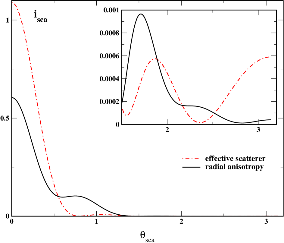
Figure 2: Scattered intensity (see Eq. (24)) versus the scattering angle at $kR_{2}=1.5$, $kd=4.0$ and $u_{1}=0.25$ for (a) effective isotropic scatterer with $m_{\mathrm{eff}}\approx 1.05127$ ($Q_{\mathrm{eff}}=0.14391$). and (b) radially anisotropic layer, $\mathbf{\hat{n}}=\mathbf{\hat{r}}$ ($Q_{Mie}=0.1439$). Insert at the upper right corner enlarges the backscattering tail.

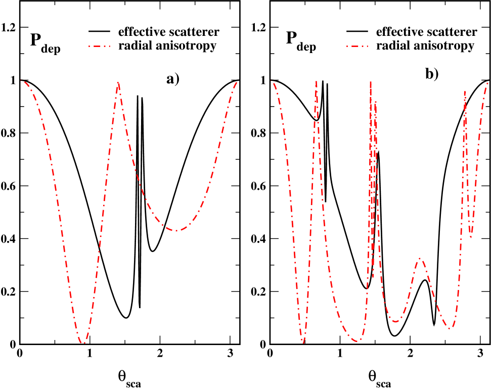
Figure 3: Depolarisation factor (see Eq. (25)) versus the scattering angle for both the radially anisotropic layer and its effective isotropic scatterer at $kR_{2}=1.5$, $u_{1}=0.25$ and (a) $kd=1.0$ ($m_{\mathrm{eff}}\approx 1.04512$, $Q_{\mathrm{eff}}=0.010724$, $Q_{rad}=0.010729$), (b) $kd=4.0$ ($m_{\mathrm{eff}}\approx 1.05127$, $Q_{\mathrm{eff}}=0.14391$, $Q_{rad}=0.1439$).

VI Discussion and Conclusions

In this paper we have developed a T-matrix approach which can describe light scattering by spherical scatterers containing optically anisotropic material arranged in an annular layer. We have confined our discussion to the two cases, which we have called, using natural language, radially and uniformly anisotropic systems. Just as in the related case when the scatterer itself is anisotropic, but the scattering material is optically isotropic, the presence of optical anisotropy affects the algebraic structure which underlies the T-matrix theory.

From a mathematical point of view, the radial and uniform anisotropies present interesting but contrasting features. Here we draw the reader’s attention to some of the most striking of these.

The simplest case is the radially anisotropic layer. Here the scattering material is locally optically anisotropic, but because of the way that the anisotropy is arranged, the scatterer itself is spherically symmetric and remains a globally optically isotropic object. The result is that there is no angular momentum mixing, although we do have to introduce the new normal mode structure (26) within the anisotropic layer.

We shall discuss quantitative results in detail in a later paper in this series. However, it is our purpose here to show briefly that the anisotropy effects can be important, even for this relatively simple case. As an example, we compare scattering by a radially anisotropic layer and a radially isotropic layer of the same dimensions, chosen in some some sense to be the best guess to an equivalent isotropic scatterer.

Specifically, we consider scattering by a scatterer with a radially anisotropic layer as discussed in section 2, with the $\epsilon_{\perp}$ within the layer matching $\epsilon$ in the core and outside the scatterer, and anisotropy coefficient $u$ inside the layer. The equivalent effective scatterer has the same dimensions, possesses an isotropic layer of refractive index $n_{\mathrm{eff}}$, so that $\epsilon_{\mathrm{eff}}$ is the dielectric constant and $m_{\mathrm{eff}}=n_{\mathrm{eff}}/n$ is the optical contrast. The refractive index $n_{\mathrm{eff}}$ is chosen so as to match scattering efficiencies of the anisotropic layer and of the effective scatterer.

We compare the angular dependence of the scattering and the depolarisation factors in the two cases. The aggregate scattering is the same, by definition. But disaggregated, we get different contributions, both when looking at angles and when looking at polarisation shifts. In Fig. 2 we compare the angular dependence of the intensities. In the case we have considered, the effective scatterer gives a much more forward scattering signature, and the relatively tiny backward scattering contribution has a very different angular structure. Likewise, we see from Fig. 3 that the depolarisation factor (25) as a function of the scattering angle, $\theta_{sca}$, is also very sensitive to the presence of anisotropy.

Given these relatively large effects for what might be thought of as minor anisotropy, there is every reason to suppose that the influence of a uniform anisotropic layer will be even more profound. In this case the light-scattering problem is not exactly soluble. The key point is that the exact solutions for uniformly anisotropic medium are known as plane waves, whereas the spherical shape of the particle requires using some kind of spherical modes.

In the case of the uniform anisotropy we have found it necessary to examine the relation between spherical harmonic expansions and plane wave solutions of Maxwell’s equations. We have found that, by choosing the appropriate basis in $\mathbf{\hat{k}}$–space, we can define ’quasi-spherical’ normal modes. These modes are exact solutions of Maxwell’s equations and as such mix different angular momentum. However, in the limit of zero anisotropy, these modes tend to familiar spherical modes. More importantly, these quasi-spherical modes turn out to be relatively easily accessible computationally. Thus, there is every reason to suppose that the strategy can be adopted in rather more complicated situations.

One such problem is the light scattering problem for a Faraday-active sphere. This problem has been treated using perturbation theory in Lacoste et al. (1998) to explain the origin of magneto-transverse light diffusion known as the “photonic Hall effect” van Tiggelen (1995); Rikken and van Tiggelen (1996).

We now try to place this problem in a more general physical context. We were first motivated by the technological problem of describing light transmission through media with liquid crystalline inclusions, and the inverse problem in which the matrix is liquid crystalline but the scatterers are isotropic. There is considerable current interest in such materials for optical applications and displays. The complete problem of light transmission through such materials not only involves the single scattering processes discussed in this paper, but also more general multiple scattering processes.

The T–matrix formalism is a natural language within which to discuss such problems. beginning with single scattering theories of the type discussed in this paper, one can in principle construct an effective medium theory using, for example, the coherent potential approximation (CPA) or coated CPA Jing et al. (1992); Soukoulis et al. (1994). These theories determine effective optical characteristics of the medium from the condition that the scattering cross section is minimal or equal to zero on average. Since this requires averaging over director orientations, it is important to use basis functions with well defined transformation properties under rotations.

This paper is the first in series of papers designed to improve understanding of scattering by optically anisotropic bodies, both singly and as components within complex anisotropic media. In the next papers in this series, we shall carry out detailed calculations using the theory presented in this paper, and compare the results with results derived using the simpler Rayleigh-Gans (RG) and Van de Hulst or Anomalous Diffraction Approximations (ADA).

Appendix A Vector spherical harmonics

In this appendix we introduce notations and definitions used throughout the paper. In addition, we relate the vector spherical harmonics and Wigner D–functions.

Let us define the vectors

$$\mathbf{e}_{\pm 1}(\mathbf{\hat{r}})=\mp(\boldsymbol{\hat{\vartheta}}\pm i\boldsymbol{\hat{\varphi}})/\sqrt{2},\quad\mathbf{e}_{0}(\mathbf{\hat{r}})\equiv\mathbf{\hat{r}}\,,$$ (52)

where $\boldsymbol{\hat{\varphi}}=(-\sin\phi,\cos\phi,0)$, $\boldsymbol{\hat{\vartheta}}=(\cos\theta\cos\phi,\cos\theta\sin\phi,-\sin\theta)$ are the unit vectors tangential to the sphere; $\phi$ and $\theta$ are Euler angles of the unit vector $\mathbf{\hat{r}}$. These vectors can be expressed in terms of the vectors of spherical basis, $\mathbf{e}_{0}\equiv\mathbf{\hat{z}}$, $\mathbf{e}_{\pm 1}=\mp(\mathbf{\hat{x}}\pm i\mathbf{\hat{y}})/\sqrt{2}$, ($\mathbf{\hat{x}},\,\mathbf{\hat{y}}$ and $\mathbf{\hat{z}}$ are the unit vectors directed along the corresponding coordinate axes) as follows:

$$\mathbf{e}_{\nu}(\mathbf{\hat{r}})=\sum_{\mu=-1}^{1}D_{\mu\nu}^{1}(\mathbf{\hat{r}})\,\mathbf{e}_{\mu},\quad\nu\in\{\pm 1,0\}\,,$$ (53)

where $D_{\mu\nu}^{\,j}(\mathbf{\hat{r}})\equiv D_{\mu\nu}^{\,j}(\phi,\theta)=\exp(-i\mu\phi)\,d_{\mu\nu}^{\,j}(\theta)$ is the Wigner $D$-function Biedenharn and Louck (1981); Gelfand et al. (1963). The following properties of the vectors (53) are easy to verify

$$(\mathbf{e}_{\nu}^{*}(\mathbf{\hat{r}})\cdot\mathbf{e}_{\mu}(\mathbf{\hat{r}}))=\delta_{\nu\mu},\quad\mathbf{e}_{\nu}(\mathbf{\hat{r}})\times\mathbf{e}_{-\nu}(\mathbf{\hat{r}})=i\nu\,\mathbf{e}_{0}(\mathbf{\hat{r}})\,.$$ (54)

The vector spherical functions ${\mathbf{Y}}_{jm}^{\,(\alpha)}$ from Eqs. (3) are expressed in terms of the vector spherical harmonics $\mathbf{Y}_{ljm}$ Biedenharn and Louck (1981) defined by

$$\mathbf{Y}_{ljm}=\sum_{\nu=-1}^{1}C_{m-\nu\,\nu\,m}^{l\,1\,j}\mathrm{Y}_{l\,m-\nu}\otimes\mathbf{e}_{\nu},\quad l=j+\delta,\quad\delta\in\{\pm 1,0\}\,,$$ (55)

where $\mathrm{Y}_{lm}=\sqrt{(2l+1)/(4\pi)}D_{m\,0}^{\,l\,*}$ is the spherical function Abramowitz and Stegun (1972) and $C_{m-\nu\,\nu\,m}^{j+\delta\,1\,j}$ denotes the Clebsch–Gordon (Wigner) coefficient,

$$\mathbf{Y}_{jm}^{(e)}=s_{j}\mathbf{Y}_{j+1\,j\,m}+c_{j}\mathbf{Y}_{j-1\,j\,m},\quad\mathbf{Y}_{jm}^{(m)}=\mathbf{Y}_{j\,j\,m}$$ (56a)

$$\mathbf{Y}_{jm}^{(o)}=-c_{j}\mathbf{Y}_{j+1\,j\,m}+s_{j}\mathbf{Y}_{j-1\,j\,m},\quad s_{j}\equiv[j/(2j+1)]^{1/2},\,c_{j}\equiv[(j+1)/(2j+1)]^{1/2}\,.$$ (56b)

Eqs. (53), (55) and the equality Biedenharn and Louck (1981)

$$C_{k_{1}k_{2}k}^{j_{1}j_{2}j}D_{mk}^{\,j}=\sum_{m_{1}m_{2}}C_{m_{1}m_{2}m}^{j_{1}\,j_{2}\,j}D_{m_{1}k_{1}}^{\,j_{1}}D_{m_{2}k_{2}}^{\,j_{2}}\,,$$ (57)

give

$$(\mathbf{Y}_{ljm}^{\,*}(\mathbf{\hat{r}})\cdot\mathbf{e}_{\nu}(\mathbf{\hat{r}}))=\left[\frac{2j+1}{4\pi}\right]^{1/2}C_{\nu}^{\,lj}D_{m\nu}^{\,j}(\mathbf{\hat{r}})\,,$$ (58)

where $C_{\nu}^{\,lj}\equiv[(2l+1)/(2j+1)]^{1/2}C_{0\,\nu\,\nu}^{\,l\,1\,j}\,$, so that the non-vanishing values of $C_{\nu}^{\,lj}$ are

$$\sqrt{2}\,C_{\nu}^{\,jj}=-\nu,\quad\sqrt{2}\,C_{\pm 1}^{\,j-1j}=-C_{0}^{\,j+1j}=c_{j},\quad\sqrt{2}\,C_{\pm 1}^{\,j+1j}=C_{0}^{\,j-1j}=s_{j}\,.$$ (59)

From Eqs. (56), (58) and (59) we express the vector spherical harmonics in terms of the Wigner D-functions as follows

$$\mathbf{Y}_{jm}^{(m)}(\mathbf{\hat{r}})=[(2j+1)/8\pi]^{1/2}\left\{D_{m,\,-1}^{j\,*}(\mathbf{\hat{r}})\,\mathbf{e}_{-1}(\mathbf{\hat{r}})-D_{m,\,1}^{j\,*}(\mathbf{\hat{r}})\,\mathbf{e}_{+1}(\mathbf{\hat{r}})\right\}\,,$$ (60a)

$$\mathbf{Y}_{jm}^{(e)}(\mathbf{\hat{r}})=[(2j+1)/8\pi]^{1/2}\left\{D_{m,\,-1}^{j\,*}(\mathbf{\hat{r}})\,\mathbf{e}_{-1}(\mathbf{\hat{r}})+D_{m,\,1}^{j\,*}(\mathbf{\hat{r}})\,\mathbf{e}_{+1}(\mathbf{\hat{r}})\right\}\,,$$ (60b)

$$\mathbf{Y}_{jm}^{(o)}(\mathbf{\hat{r}})=[(2j+1)/4\pi]^{1/2}D_{m,\,0}^{j\,*}(\mathbf{\hat{r}})\,\mathbf{e}_{0}(\mathbf{\hat{r}})\,.$$ (60c)

Note that the D-functions meet the following orthogonality relations Biedenharn and Louck (1981); Gelfand et al. (1963)

$$\langle D_{m\nu}^{\,j\,*}(\mathbf{\hat{r}})D_{m^{\prime}\nu}^{\,j^{\prime}}(\mathbf{\hat{r}})\rangle_{\mathbf{\hat{r}}}=\frac{4\pi}{2j+1}\,\delta_{jj^{\prime}}\,\delta_{mm^{\prime}}\,,$$ (61)

where $\displaystyle\langle\,f\,\rangle_{\mathbf{\hat{r}}}\equiv\int_{0}^{2\pi}\mathrm{d}\phi\int_{0}^{\pi}\sin\theta\mathrm{d}\theta\,f$. The orthogonality condition (61) and Eqs. (60a)-(60c) show that a set of vector spherical harmonics is orthonormal:

$$\langle\mathbf{Y}_{jm}^{(\alpha)\,*}(\mathbf{\hat{r}})\cdot\mathbf{Y}_{j^{\prime}m^{\prime}}^{(\beta)}(\mathbf{\hat{r}})\rangle_{\mathbf{\hat{r}}}=\delta_{jj^{\prime}}\,\delta_{mm^{\prime}}\,.$$ (62)

Appendix B Rayleigh expansions for vector plane waves

In this Appendix we comment on the vector version of the well known Rayleigh expansion (see, for example, Newton (1982)):

$$\exp(i\,\mathbf{k}\cdot\mathbf{r})=4\pi\sum_{l=0}^{\infty}\sum_{m=-l}^{l}i^{\,l}j_{l}(\rho)\,Y_{lm}(\mathbf{\hat{r}})\,Y_{lm}^{*}(\mathbf{\hat{k}}),\quad\rho\equiv kr\,.$$ (63)

Let us consider plane wave with the wave vector $\mathbf{k}\equiv k\mathbf{\hat{k}}$ and the polarisation vector $\mathbf{E}$ defined by its components, $E_{\nu}$, in the basis $\mathbf{e}_{\nu}(\mathbf{\hat{k}})$ (see Eq. (53)):

$$\mathbf{e}_{\nu}(\mathbf{\hat{k}})=\sum_{\mu=-1}^{1}D_{\mu\nu}^{1}(\mathbf{\hat{k}})\,\mathbf{e}_{\mu},\quad\mathbf{e}_{\pm 1}(\mathbf{\hat{k}})=\mp(\mathbf{e}_{x}(\mathbf{\hat{k}})\pm i\,\mathbf{e}_{y}(\mathbf{\hat{k}}))/\sqrt{2},\quad\mathbf{E}=\sum_{\nu=-1}^{1}E_{\nu}\,\mathbf{e}_{\nu}(\mathbf{\hat{k}})\,,$$ (64)

$D_{\mu\nu}^{\,j}(\mathbf{\hat{k}})\equiv D_{\mu\nu}^{\,j}(\phi_{k},\theta_{k})=\exp(-i\mu\phi_{k})\,d_{\mu\nu}^{\,j}(\theta_{k})$ is the Wigner $D$-function Biedenharn and Louck (1981); Gelfand et al. (1963) and $\phi_{k}$, $\theta_{k}$ are the azimuthal and polar angles of the unit vector $\mathbf{\hat{k}}$. The vectors $\mathbf{e}_{y}(\mathbf{\hat{k}})\equiv\boldsymbol{\hat{\varphi}}_{k}=(-\sin\phi_{k},\cos\phi_{k},0)$ and $\mathbf{e}_{x}(\mathbf{\hat{k}})\equiv\boldsymbol{\hat{\vartheta}}_{k}=(\cos\theta_{k}\cos\phi_{k},\cos\theta_{k}\sin\phi_{k},-\sin\theta_{k})$ are perpendicular to $\mathbf{\hat{k}}$.

From Eq. (63), definition of the vector spherical functions (56) and the equality (57) it is not difficult to derive the following relation

$$\mathbf{e}_{\nu}(\mathbf{\hat{k}})\exp(i\,\mathbf{k}\cdot\mathbf{r})=\sum_{j,m}[2\pi(2j+1)]^{1/2}D_{m\nu}^{j}(\mathbf{\hat{k}})\biggl{[}\sum_{l}i^{\,l}\,j_{l}(\rho)\,C_{\nu}^{\,lj}\,\mathbf{Y}_{ljm}(\mathbf{\hat{r}})\biggr{]}\,,$$ (65)

where $C_{\nu}^{\,lj}$ is defined in Eq. (59). The sum in square brackets on the right hand side of Eq. (65) can be simplified by making use of Eq. (59) and the recursion relations Abramowitz and Stegun (1972):

$$j_{j+1}+j_{j-1}=(2j+1)\rho^{-1}\,j_{j},\qquad j_{j-1}-j_{j+1}=2\frac{\mathrm{d}j_{j}}{\mathrm{d}\rho}+\rho^{-1}\,j_{j}\,.$$ (66)

The final result for transverse waves with $\nu=\pm 1$ is

$$\mathbf{e}_{\nu}\,(\mathbf{\hat{k}}) \exp(i\,\mathbf{k}\cdot\mathbf{r})=\sum_{j,m}i^{\,j-1}\,[2\pi(2j+1)]^{1/2}\,D_{m\nu}^{j}(\mathbf{\hat{k}})\cdot$$

$$\cdot\left[Dj_{j}(\rho)\mathbf{Y}_{jm}^{(e)}(\mathbf{\hat{r}})-i\nu\,j_{j}(\rho)\mathbf{Y}_{jm}^{(m)}(\mathbf{\hat{r}})+\sqrt{j(j+1)}\,\rho^{-1}\,j_{j}(\rho)\mathbf{Y}_{jm}^{(o)}(\mathbf{\hat{r}})\right]\,.$$ (67)

It can be written in the following form

$$\mathbf{e}_{x}(\mathbf{\hat{k}})\exp(i\,\mathbf{k}\cdot\mathbf{r})=\sum_{j,m}i^{j}\,[\pi(2j+1)]^{1/2}\left[D^{(y)}_{jm}(\mathbf{\hat{k}})\,\mathbf{M}^{(m)}_{jm}(\rho,\mathbf{\hat{r}})-iD^{(x)}_{jm}(\mathbf{\hat{k}})\,\mathbf{M}^{(e)}_{jm}(\rho,\mathbf{\hat{r}})\right]\,,$$ (68a)

$$\mathbf{e}_{y}(\mathbf{\hat{k}})\exp(i\,\mathbf{k}\cdot\mathbf{r})=\sum_{j,m}i^{j}\,[\pi(2j+1)]^{1/2}\left[iD^{(x)}_{jm}(\mathbf{\hat{k}})\,\mathbf{M}^{(m)}_{jm}(\rho,\mathbf{\hat{r}})+D^{(y)}_{jm}(\mathbf{\hat{k}})\,\mathbf{M}^{(e)}_{jm}(\rho,\mathbf{\hat{r}})\right]\,,$$ (68b)

where the modes $\mathbf{M}_{jm}^{(m)}$, $\mathbf{M}_{jm}^{(e)}$ are defined by Eq. (5a) and the functions $D_{jm}^{(x)}$, $D_{jm}^{(y)}$ are expressed in terms of Wigner $D$-functions in Eqs. (38a)-(38b).

Let us consider the case when the polarisation vector is directed along the $z$ axis. We derive the formulae for the following matrix elements: $\langle\,\mathbf{Y}_{jm}^{(\alpha)\,*}\cdot\mathbf{\hat{z}}\exp(i\,\mathbf{k}\cdot\mathbf{r})\,\rangle_{\mathbf{\hat{r}}}$. In order to do it, notice that the definition (55) immediately gives the following relation:

$$\mathbf{\hat{z}}\,Y_{lm}(\mathbf{\hat{r}})=\sum_{j}C^{\,l\,1\,j}_{m\,0\,m}\mathbf{Y}_{ljm}\,.$$ (69)

Then we substitute Eq. (69) into the expansion (63) multiplied by $\mathbf{\hat{z}}$ and express the vector functions $\mathbf{Y}_{ljm}$ in terms of the vector spherical harmonics $\mathbf{Y}_{jm}^{(\alpha)}$. The result reads

$$\langle\,\mathbf{Y}_{jm}^{(m)\,*}\cdot\mathbf{\hat{z}}\,\exp(i\,\mathbf{k}\cdot\mathbf{r})\,\rangle_{\mathbf{\hat{r}}}=i^{j}[4\pi(2j+1)]^{1/2}C^{\,j\,1\,j}_{m\,0\,m}\,D^{\,j}_{m0}(\mathbf{\hat{k}})\,j_{j}(\rho)\,,$$ (70a)

$$\langle\,\mathbf{Y}_{jm}^{(e)\,*}\cdot\mathbf{\hat{z}}\,\exp(i\,\mathbf{k}\cdot\mathbf{r})\,\rangle_{\mathbf{\hat{r}}}=i^{j+1}[4\pi]^{1/2}\Bigl{[}\,(2j+3)^{1/2}\,s_{j}\,C^{\,j+1\,1\,j}_{m\,0\,m}\,D^{\,j+1}_{m0}(\mathbf{\hat{k}})\,j_{j+1}(\rho)-$$

$$\phantom{\langle\,\mathbf{Y}_{jm}^{(e)\,*}\cdot\mathbf{\hat{z}}\exp(i\,\mathbf{k}\cdot\mathbf{r})\,\rangle_{\mathbf{\hat{r}}}=}-(2j-1)^{1/2}\,c_{j}\,C^{\,j-1\,1\,j}_{m\,0\,m}\,D^{\,j-1}_{m0}(\mathbf{\hat{k}})\,j_{j-1}(\rho)\Bigr{]}\,,$$ (70b)

$$\langle\,\mathbf{Y}_{jm}^{(o)\,*}\cdot\mathbf{\hat{z}}\,\exp(i\,\mathbf{k}\cdot\mathbf{r})\,\rangle_{\mathbf{\hat{r}}}=i^{j+1}[4\pi]^{1/2}\Bigl{[}\,(2j+3)^{1/2}\,c_{j}\,C^{\,j+1\,1\,j}_{m\,0\,m}\,D^{\,j+1}_{m0}(\mathbf{\hat{k}})\,j_{j+1}(\rho)+$$

$$\phantom{\langle\,\mathbf{Y}_{jm}^{(e)\,*}\cdot\mathbf{\hat{z}}\exp(i\,\mathbf{k}\cdot\mathbf{r})\,\rangle_{\mathbf{\hat{r}}}=}+(2j-1)^{1/2}\,s_{j}\,C^{\,j-1\,1\,j}_{m\,0\,m}\,D^{\,j-1}_{m0}(\mathbf{\hat{k}})\,j_{j-1}(\rho)\Bigr{]}\,.$$ (70c)

with the Wigner coefficients given by Abramowitz and Stegun (1972); Biedenharn and Louck (1981)

$$C^{\,j-1\,1\,j}_{m\,0\,m}=\left[\frac{j^{2}-m^{2}}{j(2j-1)}\right]^{1/2}\,,\,C^{\,j\,1\,j}_{m\,0\,m}=\frac{m}{\sqrt{j(j+1)}}\,,\,C^{\,j+1\,1\,j}_{m\,0\,m}=-\left[\frac{(j+1)^{2}-m^{2}}{(j+1)(2j+3)}\right]^{1/2}\,.$$ (71)

In conclusion, note that in case, when a series on the right hand side of Eq. (67) or Eqs. (70) represent a solution of the Maxwell equations (2), we can obtain another solution by replacing $j_{j}(\rho)$ with $h_{j}^{(1)}(\rho)$.

Appendix C Coefficient functions

By definition, the coefficient functions that enter the expansions (44) are the matrix elements (45). In order to deduce the corresponding formulae we need to substitute the expansions for plane waves Eqs. (68) into Eqs. (43) and make use of the matrix elements for the plane wave polarised along the $z$ axis given by Eqs. (70a)- (70c). Note that Eqs. (5) combined with the orthogonality condition for the vector spherical harmonics (62) immediately give the following relations:

$$\langle\,\mathbf{Y}_{jm}^{(m)\,*}(\mathbf{\hat{r}})\cdot\mathbf{M}_{j^{\prime}m^{\prime}}^{(\beta)}(\rho,\mathbf{\hat{r}})\,\rangle_{\mathbf{\hat{r}}}=\delta_{m,\alpha}\,\delta_{jj^{\prime}}\,\delta_{mm^{\prime}}\,j_{j}(\rho)$$ (72)

$$\langle\,\mathbf{Y}_{jm}^{(e)\,*}(\mathbf{\hat{r}})\cdot\mathbf{M}_{j^{\prime}m^{\prime}}^{(\beta)}(\rho,\mathbf{\hat{r}})\,\rangle_{\mathbf{\hat{r}}}=\delta_{e,\alpha}\,\delta_{jj^{\prime}}\,\delta_{mm^{\prime}}\,Dj_{j}(\rho)\,.$$ (73)

Below we write the resulting expressions for the matrix elements that correspond to transverse components of the wave functions (43).

$$p_{jj^{\prime};\,m}^{\,(m,\,m)}(\rho)=N_{jj^{\prime}}\,\langle\,d^{\,(y;\,y)}_{j^{\prime}j;\,m}\,j_{j}(\rho_{e})+d^{\,(x;\,x)}_{j^{\prime}j;\,m}\,j_{j}(\rho)\,\rangle_{\theta_{k}}+\Delta\,p_{jj^{\prime};\,m}^{\,(m,\,m)}(\rho)\,,$$ (74)

$$p_{jj^{\prime};\,m}^{\,(m,\,e)}(\rho)=i\,N_{jj^{\prime}}\,\langle\,d^{\,(x;\,y)}_{j^{\prime}j;\,m}\,j_{j}(\rho_{e})+d^{\,(y;\,x)}_{j^{\prime}j;\,m}\,j_{j}(\rho)\,\rangle_{\theta_{k}}+\Delta\,p_{jj^{\prime};\,m}^{\,(m,\,e)}(\rho)\,,$$ (75)

$$p_{jj^{\prime};\,m}^{\,(e,\,m)}(\rho)=-i\,N_{jj^{\prime}}\,\langle\,d^{\,(y;\,x)}_{j^{\prime}j;\,m}\,Dj_{j}(\rho_{e})+d^{\,(x;\,y)}_{j^{\prime}j;\,m}\,Dj_{j}(\rho)\,\rangle_{\theta_{k}}+\Delta\,p_{jj^{\prime};\,m}^{\,(m,\,e)}(\rho)\,,$$ (76)

$$p_{jj^{\prime};\,m}^{\,(e,\,e)}(\rho)=N_{jj^{\prime}}\,\langle\,d^{\,(x;\,x)}_{j^{\prime}j;\,m}\,Dj_{j}(\rho_{e})+d^{\,(y;\,y)}_{j^{\prime}j;\,m}\,Dj_{j}(\rho)\,\rangle_{\theta_{k}}+\Delta\,p_{jj^{\prime};\,m}^{\,(e,\,e)}(\rho)\,,$$ (77)

$$q_{jj^{\prime};\,m}^{\,(m,\,m)}(\rho)=N_{jj^{\prime}}\,\langle\,d^{\,(x;\,x)}_{j^{\prime}j;\,m}\,j_{j}(\rho_{e})\,n_{e}^{-1}+d^{\,(y;\,y)}_{j^{\prime}j;\,m}\,j_{j}(\rho)\,\rangle_{\theta_{k}}\,,$$ (78)

$$q_{jj^{\prime};\,m}^{\,(m,\,e)}(\rho)=i\,N_{jj^{\prime}}\,\langle\,d^{\,(y;\,x)}_{j^{\prime}j;\,m}\,j_{j}(\rho_{e})\,n_{e}^{-1}+d^{\,(x;\,y)}_{j^{\prime}j;\,m}\,j_{j}(\rho)\,\rangle_{\theta_{k}}\,,$$ (79)

$$q_{jj^{\prime};\,m}^{\,(e,\,m)}(\rho)=-i\,N_{jj^{\prime}}\,\langle\,d^{\,(x;\,y)}_{j^{\prime}j;\,m}\,Dj_{j}(\rho_{e})\,n_{e}^{-1}+d^{\,(y;\,x)}_{j^{\prime}j;\,m}\,Dj_{j}(\rho)\,\rangle_{\theta_{k}}\,,$$ (80)

$$q_{jj^{\prime};\,m}^{\,(e,\,e)}(\rho)=i\,N_{jj^{\prime}}\,\langle\,d^{\,(y;\,y)}_{j^{\prime}j;\,m}\,Dj_{j}(\rho_{e})\,n_{e}^{-1}+d^{\,(x;\,x)}_{j^{\prime}j;\,m}\,Dj_{j}(\rho)\,\rangle_{\theta_{k}}\,,$$ (81)

where $N_{jj^{\prime}}\equiv\dfrac{i^{j^{\prime}-j}}{8}[(2j+1)(2j^{\prime}+1)]^{1/2}$ and $d^{\,(\alpha;\,\beta)}_{jj^{\prime};\,m}\equiv d^{\,(\alpha)}_{jm}(\theta_{k})d^{\,(\beta)}_{j^{\prime}m}(\theta_{k}),\quad\alpha,\,\beta\in\{x,\,y,\,z\}$. The terms $\Delta\,p_{jj^{\prime};\,m}^{\,(\alpha,\,\beta)}(\rho)$ are given by

$$\Delta\,p_{jj^{\prime};\,m}^{\,(m,\,m)}(\rho)=N_{jj^{\prime}}\,\frac{2m}{\sqrt{j(j+1)}}\,r_{jj^{\prime};\,m}^{\,(z,\,x)}(\rho)\,,$$ (82)

$$\Delta\,p_{jj^{\prime};\,m}^{\,(m,\,e)}(\rho)=N_{jj^{\prime}}\,\frac{2m}{\sqrt{j(j+1)}}\,r_{jj^{\prime};\,m}^{\,(z,\,y)}(\rho)\,,$$ (83)

$$\Delta\,p_{jj^{\prime};\,m}^{\,(e,\,m)}(\rho)=N_{jj^{\prime}}\,\frac{-2\,i}{2j+1}\,\biggl{\{}[j((j+1)^{2}-m^{2})/(j+1)]^{1/2}\,r_{j+1\,j^{\prime};\,m}^{\,(z,\,y)}(\rho)-$$

$$\phantom{\Delta\,p_{jj^{\prime};\,m}^{\,(e,\,m)}(\rho)=N_{jj^{\prime}}\,\frac{-2\,i}{2j+1}\,}-[(j+1)(j^{2}-m^{2})/j]^{1/2}\,r_{j-1\,j^{\prime};\,m}^{\,(z,\,y)}(\rho)\biggr{\}}\,,$$ (84)

$$\Delta\,p_{jj^{\prime};\,m}^{\,(e,\,e)}(\rho)=N_{jj^{\prime}}\,\frac{2}{2j+1}\,\biggl{\{}[j((j+1)^{2}-m^{2})/(j+1)]^{1/2}\,r_{j+1\,j^{\prime};\,m}^{\,(z,\,x)}(\rho)-$$

$$\phantom{\Delta\,p_{jj^{\prime};\,m}^{\,(e,\,m)}(\rho)=N_{jj^{\prime}}\,\frac{-2\,i}{2j+1}\,}-[(j+1)(j^{2}-m^{2})/j]^{1/2}\,r_{j-1\,j^{\prime};\,m}^{\,(z,\,x)}(\rho)\biggr{\}}\,,$$ (85)

where

$$r_{j\,j^{\prime};\,m}^{\,(z,\,\alpha)}(\rho)=\frac{u}{u+1}\langle\,d^{\,(\alpha;\,z)}_{j^{\prime}j;\,m}(\theta_{k})\,j_{j}(\rho_{e})\,\sin\theta_{k}\,\rangle_{\theta_{k}}\,.$$ (86)

Expressions for $\tilde{p}_{jj^{\prime};\,m}^{\,(\alpha,\,\beta)}(\rho)$ and $\tilde{q}_{jj^{\prime};\,m}^{\,(\alpha,\,\beta)}(\rho)$ can be derived from Eqs. (74)–(86) by replacing spherical Bessel functions of the first kind $j_{j}(x)$ with spherical Bessel functions of the third kind $h_{j}^{(1)}(x)$.

The coefficient functions $p_{jj^{\prime};\,m}^{\,(\alpha,\,\beta)}$ and $q_{jj^{\prime};\,m}^{\,(\alpha,\,\beta)}$ are diagonal, $\propto\delta_{\alpha,\,\beta}\,\delta_{jj^{\prime}}$, in the limit of weak anisotropy, $u\to 0$. It can be seen from orthogonality condition (61) that provides the orthogonality conditions for $d$-functions defined by Eqs. (38a)-(38b) in the following form

$$\langle\,d^{\,(x;\,x)}_{j^{\prime}j;\,m}+d^{\,(y;\,y)}_{j^{\prime}j;\,m}\,\rangle_{\theta_{k}}=\frac{8}{2j+1}\,\delta_{jj^{\prime}}\,,$$

$$\langle\,d^{\,(x;\,y)}_{j^{\prime}j;\,m}+d^{\,(y;\,x)}_{j^{\prime}j;\,m}\,\rangle_{\theta_{k}}=0\,.$$ (87)

References

• Mie (1908) G. Mie, Ann. Phys. (Leipzig) 25, 377 (1908).
• Asano and Yamamoto (1975) S. Asano and G. Yamamoto, Appl. Opt. 14, 29 (1975).
• Roth and Digman (1973) J. Roth and M. Digman, J. Opt. Soc. Am. 63, 308 (1973).
• Lange and Aragon (1990) B. Lange and S. Aragon, J. Chem. Phys. 92, 4643 (1990).
• Hahn and Aragon (1994) D. Hahn and S. Aragon, J. Chem. Phys. 101, 8409 (1994).
• Karacali et al. (1997) H. Karacali, S. Risseler, and K. Ferris, Phys. Rev. B 56, 4286 (1997).
• Kiselev et al. (2000a) A. Kiselev, V. Reshetnyak, and T. Sluckin, in Proc. Bianisotropics’2000, edited by A. Barbosa and A. Topa (8th Intern. Conf. on Electromagnetics of Complex Media, Lisbon, Portugal, 2000a), pp. 343–346.
• Kiselev et al. (2000b) A. Kiselev, V. Reshetnyak, and T. Sluckin, Opt. Spectrosc. 89(6), 907 (2000b).
• Newton (1982) R. Newton, Scattering Theory of Waves and Particles (Springer, Heidelberg, 1982), 2nd ed.
• Ishimaru (1978) A. Ishimaru, Wave Propagation and Scattering in Random Media (Academic Press, New York, 1978).
• Kreuzer and Eidenschink (1996) M. Kreuzer and R. Eidenschink, in Liquid Crystals in Complex Geometries, edited by G. Crawford and S. Žumer (Taylor & Francis, London, 1996), chap. 15.
• Bellini et al. (1998) T. Bellini, N. Clark, V. Degiorgio, F. Mantegazza, and G. Natale, Phys. Rev. E 57, 2996 (1998).
• Mishchenko et al. (1996) M. Mishchenko, L. Travis, and D. Mackowski, J. of Quant. Spectr. & Radiat. Transf. 55, 535 (1996).
• Mishchenko et al. (2000) M. Mishchenko, J. Hovenier, and L. Travis, eds., Light Scattering by Nonspherical Particles: Theory, Measurements and Applications (Academic Press, New York, 2000).
• Boren and Huffman (1983) C. Boren and D. Huffman, Absorption and Scattering of Light by Small Particles (Wiley-Interscience, New York, 1983).
• Žumer and Doane (1986) S. Žumer and J. Doane, Phys. Rev. A 34, 3373 (1986).
• Žumer (1988) S. Žumer, Phys. Rev. A 37, 4006 (1988).
• Biedenharn and Louck (1981) L. Biedenharn and J. Louck, Angular Momentum in Quantum Physics (Addison–Wesley, Reading, Massachusetts, 1981).
• Abramowitz and Stegun (1972) M. Abramowitz and I. Stegun, eds., Handbook of Mathematical Functions (Dover, New York, 1972).
• Gelfand et al. (1963) I. Gelfand, R. Minlos, and Z. Shapiro, Representations of Rotation and Lorenz Groups and Their Applications (Pergamon Press, Oxford, 1963).
• Born and Wolf (1980) M. Born and E. Wolf, Principles of Optics (Pergamon Press, Oxford, 1980), 2nd ed.
• Landau and Lifshitz (1984) L. Landau and E. Lifshitz, Elecrtodynamics of Continuous Media (Pergamon, Oxford, 1984).
• Lax and Nelson (1971) M. Lax and D. Nelson, Phys. Rev. B 4, 3694 (1971).
• Stark and Lubensky (1997) H. Stark and T. Lubensky, Phys. Rev. E 55, 514 (1997).
• Lacoste et al. (1998) D. Lacoste, B. van Tiggelen, G. Rikken, and A. Sparenberg, J. Opt. Soc. Am. A 15, 1636 (1998).
• van Tiggelen (1995) B. van Tiggelen, Phys. Rev. Lett. 75, 422 (1995).
• Rikken and van Tiggelen (1996) G. Rikken and B. van Tiggelen, Nature 381, 54 (1996).
• Jing et al. (1992) X. Jing, P. Sheng, and M. Zhou, Phys. Rev. A 46, 6513 (1992).
• Soukoulis et al. (1994) C. Soukoulis, S. Datta, and E. Economou, Phys. Rev. B 49, 3800 (1994).