Excitons in a Photosynthetic Light-Harvesting System: A Combined Molecular Dynamics/Quantum Chemistry and Polaron Model Study

Abstract

The dynamics of pigment-pigment and pigment-protein interactions in light-harvesting complexes is studied with a novel approach that combines molecular dynamics simulations with quantum chemistry calculations and a polaron model analysis. The molecular dynamics simulation of light-harvesting complexes was performed on an 87,055 atom system comprised of an LH-II complex of Rhodospirillum molischianum embedded in a lipid bilayer and surrounded with appropriate water layers. The simulation provided information about the extent and timescales of geometrical deformations of pigment and protein residues at physiological temperatures, revealing also a pathway of a water molecule into the B800 binding site, as well as increased dimerization within the B850 BChl ring, as compared to the dimerization found for the crystal structure. For each of the 16 B850 BChls we performed 400 ab initio quantum chemistry calculations on geometries that emerged from the molecular dynamical simulations, determining the fluctuations of pigment excitation energies as a function of time. From the results of these calculations we construct a time-dependent Hamiltonian of the B850 exciton system from which we determine within linear response theory the absorption spectrum. Finally, a polaron model is introduced to describe both the excitonic and coupled phonon degrees of freedom by quantum mechanics. The exciton-phonon coupling that enters into the polaron model, and the corresponding phonon spectral function are derived from the molecular dynamics and quantum chemistry simulations. The model predicts that excitons in the B850 bacteriochlorophyll ring are delocalized over five pigments at room temperature. Also, the polaron model permits the calculation of the absorption spectrum of the B850 excitons from the sole knowledge of the autocorrelation function of the excitation energies of individual BChls, which is readily available from the combined molecular dynamics and quantum chemistry simulations. The obtained result is found to be in good agreement with the experimentally measured absorption spectrum.

I Introduction

Life on earth is sustained through photosynthesis. The initial step of photosynthesis involves absorption of light by the so-called light-harvesting antennae complexes, and funneling of the resulting electronic excitation to the photosynthetic reaction center [1, 2, 3, 4]. In case of purple bacteria, light-harvesting complexes are ring-shaped aggregates of proteins that contain two types of pigments, bacteriochlorophylls (BChls) and carotenoids.

Recent solution of the atomic level structure of the light-harvesting complex II (LH-II) of two species of purple bacteria, Rhodopseudomonas (Rps.) acidophila [5] and Rhodospirillum (Rs.) molischianum [6], has opened the door to an understanding of the structure-function relationship in these proteins. Fig. 1 shows the structure of LH-II of Rs. molischianum in its membrane-water environment. LH-II is an octamer, consisting of eight $\alpha$- and eight $\beta$- protein subunits which bind non-covalently the following pigments: eight BChls that absorb at 800 nm and are referred to as B800 BChls, 16 BChls that absorb at 850 nm, and are referred to as B850 BChls, and eight carotenoids which absorb at 500 nm. The pigment system of LH-II is shown in Fig. 2. The difference in absorption maxima between various pigments funnels electronic excitation within LH-II; pigments with higher excitation energy pass on their excitation to the pigments with lower excitation energy. As a result, energy absorbed by the carotenoids, or the B800 BChls, is funneled into the B850 ring [7]. The B850 ring, in turn, transfers the electronic excitation to a BChl ring in another light-harvesting complex, LH-I, which is directly surrounding the photosynthetic reaction center. The B850 ring, thus, serves as a link in a chain of excitation transfer steps which result ultimately in excitation of the photosynthetic reaction center [7].

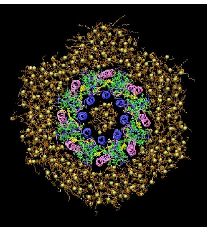
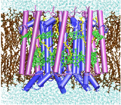
FIG. 1.: Top: Top view of the LH-II octameric complex of Rs. molischianum [6] embedded into a lipid bilayer that fits into a hexagonal unit cell. The simulated system consists of an infinite, periodic repeat of this unit cell. The lipids, 267 molecules of palmitoyloleoylphosphatidylcholine (POPC), are shown in brown, with phosphorus atoms in yellow. The $\alpha$- and $\beta$- protein subunits of LH-II are shown in blue and magenta, respectively; bacteriochlorophylls are shown in green, carotenoids in yellow. Bottom: Side view of LH-II in the lipid-water environment. For clarity, the front half of the lipids is not displayed. The color code is the same as for the top view; however, the $\alpha$-helical segments of the protein subunits are rendered as cylinders. Water molecules are shown in light-blue. One can recognize two ring-shaped clusters of BChl molecules (green). A ring of eight (only four visible) BChls at the top is formed by the B800 BChls; a ring of sixteen BChls (only partially visible) at the bottom is formed by 16 B850 BChls. (Produced with the program VMD [8]).

The B800 and B850 BChls have in common a tetrapyrol moiety that includes the electronically excited $\pi$-electron system; they differ only in the length of their phytyl chain [6]. The difference in the absorption maxima arises through the difference in their ligation sites. Protein residues at the ligation site, especially aromatic, charged or polar ones, as well as hydrogen bonds between pigment and protein residues can shift the absorption maxima of pigments [9]. However, the difference in absorption maxima is also evoked through excitonic interactions between the B850 BChls [10]. The $\pi$-electron systems of neighboring B850 BChls are in van der Waals contact [6], giving rise to strong couplings between their electronic excitations. This coupling leads to coherently delocalized electronic excitations, so-called excitons [11].

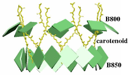
FIG. 2.: Side view of the arrangement of BChl and carotenoid pigments in LH-II with the protein components of LH-II stripped away. BChls are presented as green squares. Sixteen B850 BChls are arranged in the bottom ring and eight B800 BChls in the top ring. Eight carotenoids, shown in yellow, were identified in the crystal structure at the positions shown (produced with the program VMD [8]).

What is intriguing about the light-harvesting complexes of purple bacteria is their circular symmetry: LH-II of Rs. molischianum is an octamer; LH-II of Rps. acidophila is a nonamer [5]; electron density projection maps indicate that LH-I of Rs. rubrum is a hexadecamer [12]. This poses the question whether the circular shape plays a functional role. In [7] we have constructed an effective Hamiltonian to describe the excitons formed by the Q_y excitations of B850 BChls. The Hamiltonian was assumed to exhibit a perfect 8-fold symmetry axis for a ring of 16 B850 BChls. In the case of such ideal symmetry, stationary states, the excitons, have optical properties characteristic of the symmetry. The dipole strength is unequally distributed among the excitonic states. In fact, two degenerate excitonic states carry almost all of the dipole strength. This property facilitates overall absorption, since the two degenerate states each absorb with the strength of eight BChls. Furthermore, an energy trap is formed; the lowest exciton state carries very small dipole strength, making fluorescence negligible. As a result, this state, when populated through thermal redistribution, traps effectively the excitation energy. However, this scenario holds only as long as the symmetry is not broken significantly.

Interactions of BChls with its protein environment in LH-II of Rs. molischianum, together with thermal motions, give rise to static and dynamic disorder which manifests itself through distortions of the 8-fold symmetry. The classification of disorder is based on the time-scale of protein thermal motions compared to the characteristic times of absorption, fluorescence, and excitation transfer. If the protein motion is slow compared to the latter processes, the effect of the environment can be considered as static; otherwise, the effect is dynamic. The nature of the disorder (static or dynamic) is reflected in the line-shape functions characterizing the energy dependence of optical absorption and emission processes. It is important to know these functions when studying energy transfer between two molecules since their overlap determines the transfer rate.

The disorder in LH-II affects the energy level structure and optical properties of excitonic states, that in turn influence absorption, fluorescence and excitation transfer. To understand the dynamics of LH-II it is necessary to quantify the extent of disorder. One measure of the effect of disorder is the exciton delocalization length (see for example [13, 14]). For a completely symmetric aggregate at temperature T = 0 K, the exciton delocalization length is equal to the total number of BChls, in the case of LH-II of Rs. molischianum, sixteen. With increased disorder the coherence of the delocalized states is lost, and the excitons become confined to a smaller number of BChls [14].

Exciton delocalization in light-harvesting complexes of purple bacteria has been a subject of extensive experimental study. Non-linear absorption [15], circular dichroism [16], femtosecond transient absorption [17], fluorescence [18], pump-probe [19], photon echo [20] and single-molecule experiments [21], techniques have been employed to study exciton delocalization length, resulting in vastly different estimates which range from delocalization over two BChls [22], to delocalization over the entire ring [15]. One of the obvious explanations for different estimates of exciton delocalization are differences in the definition of observables as well as differences in the temperature at which experiments were performed.

It appears desirable to complement the experimental observations of the effect of disorder on the exciton system of light harvesting proteins by simulations. Such simulations can provide a detailed, atomic level picture of the disorder and its effect. However, the required simulations are extremely demanding. On the one hand, one needs to simulate the classical motion of light harvesting proteins in their natural lipid-water environment under periodic boundary conditions (to avoid finite size effects) and under the influence of full electrostatics (dipolar forces play a key role in membrane systems). On the other hand, one needs to carry out, in combination with the classical simulations, quantum chemical calculations that account for the coupling between protein dynamics and electronic properties of the BChl systems. Fortunately, the necessary calculations have become feasible recently. Naturally, limitations in regard to short sampling times and still rather crude quantum chemical descriptions still exist. Nevertheless, a description of static and dynamic disorder based on computer simulations, rather than on ad hoc assumptions, would constitute a great step forward in our understanding of the light harvesting apparatus in photosynthesis. This is particularly true since the apparatus is based on aggregates of numerous pigments, the functional properties of which are sensitive to thermal fluctuations. A model that includes complete information on the actual disorder and its effect on the electronic properties provides also an opportunity to improve the analysis of experimental data.

In this paper we investigate the effect of thermal disorder on excitons in LH-II at room temperature. We employ a combined molecular dynamics/quantum chemistry approach to establish an effective time-dependent Hamiltonian for the Q_y excitations of B850 BChls. This Hamiltonian is used in a quantum mechanical treatment from which the spectral characteristics of the B850 BChl system results. The description is then recast into a polaron model that treats both nuclear motion and electronic degrees of freedom on an equal (quantum mechanical) footing. The theory underlying our analysis of spectral properties is outlined in chapter II; the methods employed for combined molecular dynamics/quantum chemistry simulations are described in chapter III; results, together with the theory of the polaron model, are presented and discussed in chapters IV and V. Conclusions are stated in chapter VI.

II Theory and Computation of Spectral Properties

We describe the electronic properties of the B850 BChls in LH-II under the assumption that the rest of LH-II, i.e., protein, B800 BChls, and lycopenes, play merely the role of a thermal bath. The total Hamiltonian for this BChl-bath system can be written

$$\hat{H}\;=\;\hat{H}_{BChl}\;+\;\hat{H}_{BChl-Bath}\;+\;\hat{H}_{Bath}\,.$$ (1)

The individual Hamiltonians in Eq. (1) can be further decomposed as

$$\hat{H}_{BChl}\;=\;T_{el}\;+\;T_{nuc}\;+\;V_{el-el}\;+\;V_{el-nuc}\;+\;V_{nuc-nuc}$$ (2)

$$\hat{H}_{BChl-Bath}\;=\;V_{el-Bath}\;+\;V_{nuc-Bath}$$ (3)

$$\hat{H}_{Bath}\;=\;T_{Bath}\;+\;V_{Bath-Bath}\;.$$ (4)

The indices of the quantities introduced in Eqs.(1-4) are chosen in an obvious manner to define the partial Hamiltonians sufficiently. Due to the large mass difference of electrons and nuclei, we separate BChl degrees of freedom into “light” and “heavy”ones, i.e., electronic and nuclear. We introduce the following set of indices; $r=(\vec{r}_{1},\vec{r}_{2},\cdots,\vec{r}_{N_{el}})$, for all of the electronic degrees of freedom of BChl; $R=(\vec{R}_{1},\vec{R}_{2},\cdots,\vec{R}_{N_{nuc}})$, for all of the nuclear degrees of freedom of BChl; and $Z=(\vec{Z}_{1},\vec{Z}_{2},\cdots,\vec{Z}_{N_{Bath}})$, for all of the bath degrees of freedom. Index $Z$ labels bath atoms as a whole, i.e., the splitting of the bath degrees of freedom into nuclear and electronic is neglected.

According to the Born-Oppenheimer (BO) approximation [23] we assume that the electrons move adiabatically in a potential that depends parametrically on the atomic coordinates of BChl and bath. If $\hat{H}_{BChl}$ describes a single BChl, the above approximation applies well. The energy gap between ground state and lowest singlet excited state Q_y, the relevant states, measures about 1.5 eV, which is too large for vibrationally induced transitions to occur, i.e., the BO approximation holds well. However, if $\hat{H}_{BChl}$ describes an entire B850 BChl ring (comprised of 16 BChls), energy gaps between 16 excitonic states are much smaller and vibrations might induce transitions between these states. Therefore, we will assume that $\hat{H}_{BChl}$ describes only one of the B850 BChl, while the remaining B850 BChls will join the bath system. From this description we will derive the characteristics that enter into a so-called polaron model which describes vibronic coupling to the electronic degrees of freedom, treating both excitons and vibrations quantum mechanically.

Within the framework of the BO approximation we construct the Schrödinger equation for the electronic wavefunction, which depends parametrically on the nuclear coordinates $R$ and coordinates of bath atoms $Z$ [23]

$$\hat{H}^{i}_{el}(R,Z)\,\phi^{i}_{a}(r_{i};R,Z)\;=\;\epsilon^{i}_{a}(r_{i};R,Z)\,\phi^{i}_{a}(r_{i};R,Z)\;.$$ (5)

Here $\hat{H}^{i}_{el}$ is the electronic Hamiltonian of the $i$-th B850 BChl

$$\hat{H}^{i}_{el}(R,Z)\;=\;T_{el}\;+\;V_{el-el}\;+\;V_{el-nuc}\;+\;V_{el-Bath}\;,$$ (6)

$\epsilon^{i}_{a}$ and $\phi^{i}_{a}$ are the $a$-th eigenvalue and eigenvector, respectively, of the $i$-th BChl. At the moment we are only interested in the ground and the $Q_{y}$ electronic state of BChl. The electronic problem stated in Eqs. (5,6) has been solved with the quantum chemistry package Gaussian 98 [24], as explained in section III.

The equations of motions of the nuclear and bath degrees of freedom are solved in the framework of the BO approximation, i.e., neglecting the non-adiabatic coupling [23, 25]

$$\hat{H}_{nuc+Bath}(R,Z)=T_{nuc}\;+\;T_{Bath}\,+\;V_{nuc-nuc}(R)$$ (7)

$$+\;V_{Bath-Bath}(Z)+V_{nuc-Bath}(R,Z)+\epsilon^{a}_{i}(R,Z)\;.$$ (8)

Dynamics of the nuclear and bath degrees of freedom can be described through classical molecular dynamics simulations. The trajectory of nuclear and bath coordinates ($R(t_{k}),Z(t_{k})$) for various simulation times $t_{k}$ can be generated, as described also in section III. By treating $R(t_{k})$ and $Z(t_{k})$ as parameters, energies of the ground state, $\epsilon^{i}_{0}(t_{k})$, and of the excited Q_y state, $\epsilon^{i}_{Q_{y}}(t_{k})$, will be calculated for each BChl $i$, $i=1,2,\ldots,16$.

A Time-dependent Hamiltonian of the B850 Ring

We construct now the time-dependent electronic Hamiltonian $\hat{H}(t)$ of the BChl ring. The time-dependence of $\hat{H}(t)=\hat{H}(R(t),Z(t))$ arises through vibrational motions of the nuclear and bath degrees of freedom. The electronic Hamiltonian is expressed in the basis comprised of the ground state of the B850 ring

$$|0\rangle\;=\;\prod_{i}|\phi^{i}_{0}\rangle$$ (9)

and of the sixteen Q_y excitations of individual BChls

$$|i\rangle\;=\;|\phi^{i}_{Q_{y}}\rangle\prod_{j\neq i}|\phi^{j}_{0}\rangle\;,$$ (10)

where $|\phi^{i}_{0}\rangle$ and $|\phi^{i}_{Q_{y}}\rangle$ denote the ground and the $Q_{y}$ excited state of the $i$th BChl. It is assumed that the states defined in (9, 10) are time-independent and orthonormal, i.e., $\langle i|j\rangle\,=\,\delta_{i,j}$ for $i,j\,=\,0,1,\ldots$. The Hamiltonian now reads [23]

$$\hat{H}(t)\;=\;H_{0}(t)|0\rangle\langle 0|\;+\;\hat{H}_{1}(t)\sum_{i=1}^{16}|i\rangle\langle i|\;.$$ (11)

where

$$H_{0}(t)\;=\;\sum_{i}\epsilon^{i}_{0}(t)$$ (12)

and

$$\hat{H}_{1}(t)=H_{0}(t) + \sum_{i,j=1}^{16}[\,\delta_{i,j}(\epsilon^{i}_{Q_{y}}(t)-\epsilon^{i}_{0}(t))$$ (13)

$$+ \,(1\,-\delta_{i,j})\,W_{i,j}(t)]\,|i\rangle\langle j|\,]\;.$$ (14)

The right-hand term in Hamiltonian (13) describes the interactions between Q_y excitations of all the BChls of the B850 ring, and can be rewritten as

$$\hat{H}(t)^{exc}=\pmatrix{\epsilon_{1}(t)&&&&&&\cr&\epsilon_{2}(t)&&&&&\cr&&.&&W_{ij}(t)&&\cr&&&.&&&\cr&&&&.&&\cr&&W_{ji}(t)&&&.&\cr&&&&&&\epsilon_{16}(t)\cr}\;.$$ (15)

Here $\epsilon_{i}(t)={\epsilon^{i}_{Q_{y}}(t)-\epsilon^{i}_{0}(t)}$ and $W_{i,j}(t)$ is the induced dipole – induced dipole coupling between BChls $i$ and $j$

$$W_{ij}(t)\;=\;C\left(\,{\vec{n}_{i}(t)\cdot\vec{n}_{j}(t)\over{r_{ij}(t)}^{3}}-{3(\vec{r}_{ij}(t)\cdot\vec{n}_{i}(t))\;(\vec{r}_{ij}(t)\cdot\vec{n}_{j}(t))\over{r_{ij}(t)}^{5}}\,\right)\;,$$ (16)

where $\vec{n}_{j}(t)$ are unit vectors describing the direction of the transition dipole moments $\vec{d}_{j}$ of the ground state $\rightarrow$ Q_y state transition of the $j$-th BChl, i.e., $\vec{n}_{j}(t)=\vec{d}_{j}(t)/|\vec{d}_{j}(t)|$, and it points from N atom of pyrol II to the N atom of pyrol IV in BChl $j$ at snapshot $t$. $\vec{r}_{jk}(t)$ connects the coordinates of Mg atoms of BChl $j$ and BChl $k$ at time $t$. C is a constant proportional to the square of the magnitude of the transition dipole, assumed to be constant, and is set to 21.12 Å${}^{3}\,eV$. The latter value is obtained when a computationally determined value of C = 64.38 Å${}^{3}\,eV$ [7], which corresponds to a transition dipole moment of 11 D, is rescaled to match the experimental value 6.3 D [26] of the transition dipole moment. For simplicity we assume that the coupling between neighboring (and all other) BChls is given by $W_{ij}(t)$, even though the short distance between neighboring BChls does not justify limitation to only the leading term of a multipole expansion. We note, however, that the amplitude of calculated variations of $W_{ij}(t)$ is two orders of magnitude smaller than that for the diagonal matrix elements $\epsilon_{i}(t)$ (see results section), and that the error involved in the treatment will not alter the qualitative behavior of the system.

The formal solution of the time-dependent Schrödinger equation for Hamiltonian $\hat{H}(t)^{exc}$ [25]

$$i\,{\hbar}\,\frac{\partial|\Psi(t)\rangle^{exc}}{\partial t}\;=\;\hat{H}(t)^{exc}\,|\Psi(t)\rangle^{exc}\;,$$ (17)

can be written

$$|\Psi(t)\rangle^{exc}\;=\;\tilde{U}(t,t_{0})\,|\Psi(t_{0})\rangle^{exc}\;,$$ (18)

where $\tilde{U}(t,t_{0})$ is the time-development operator. By dividing the time interval $[t,t_{0}]$ into $N$ smaller intervals, $\tilde{U}(t,t_{0})$ can be written $(t\,=\,t_{N})$

$$\tilde{U}(t,t_{0})\;=\;\tilde{U}(t_{N},t_{N-1})\,\tilde{U}(t_{N-1},t_{N-2})\,\cdots\,\tilde{U}(t_{1},t_{0}).$$ (19)

If $N$ is sufficiently large, $\hat{H}(t)^{exc}$ can be considered to be constant in each time interval $[t_{k},t_{k+1}]$, i.e., for $\hat{H}(t)^{exc}=\hat{H}(t_{k})^{exc}$ for $t\,\in\,[t_{k},t_{k+1}]$. The time-development operator $\tilde{U}(t_{k+1},t_{k})$ can then be determined as

$$\tilde{U}(t_{k+1},t_{k}) = \sum_{m}\exp\left[-{i\over\hbar}E_{m}^{(k)}\,(t_{k+1}-t_{k})\right]$$ (21)

$$\times||m\rangle^{(k)}\,{}^{(k)}\langle m||\;.$$

Here $E_{m}^{(k)}$ and $||m\rangle^{(k)}$ are eigenvalues and eigenvectors of $\hat{H}(t_{k})^{exc}$. The eigenvectors can be expanded

$$||m\rangle^{(k)}\;=\;\sum_{j}\,c_{j,m}^{(k)}\,|j\rangle.$$ (22)

The time development operator $\tilde{U}(t,t_{0})$ can be determined from combined molecular dynamics/quantum chemistry data. Molecular dynamics simulation will result in a trajectory of coordinates $R(t_{k})$, $Z(t_{k})$. Based on the coordinates $R(t_{k})$, the values of $W_{i,j}(t_{k})$ in Hamiltonian (15) can be calculated through Eq. (16). The diagonal matrix elements, $\epsilon_{i}(t_{k})$, are determined with the quantum chemistry program Gaussian 98 [24], as described in the methods section.

The Hamiltonian $\hat{H}(t_{k})^{exc}$ can be diagonalized, and the excitation energies $E_{n}^{(k)}$, and eigenvectors $||m\rangle^{(k)}$ determined. Calculation of $\tilde{U}(t,t_{0})$ and $|\Psi(t)\rangle^{exc}$ follows straightforwardly from Eqs. (18,19,21).

The time development operator $U(t,t_{0})$ for the entire Hamiltonian (11), $\hat{H}(t)$, can be easily calculated from $\tilde{U}(t,t_{0})$. Exploiting orthogonality between ground and excited states ($\langle 0|i\rangle\,=\,0$), and noting that $H_{0}(t)$ appearing in Eqs. (11,12,13) is a c-number, one can express

$$U(t,t_{0}) = \exp\left[-{i\over\hbar}\int_{t_{0}}^{t}\,dt^{\prime}H_{0}(t^{\prime})\right]$$ (24)

$$\times\left[|0\rangle\langle 0|\;+\;\sum_{ij}[\tilde{U}(t,t_{0})]_{ij}|i\rangle\langle j|\right]\;.$$

The solution of the time-dependent Schrödinger equation associated with $\hat{H}(t)$ is

$$|\Psi(t)\rangle=U(t,t_{0})|\Psi(t_{0})\rangle\;.$$ (25)

B Absorption spectrum of a coupled chlorophyll aggregate

In the following we will derive an expression for the absorption coefficient for the B850 ring, in the framework of linear response theory. We note that within the dipole approximation the total Hamiltonian $\hat{H}_{tot}$ describing the BChl system and its interaction with the radiation field can be chosen

$$\hat{H}_{tot}\;=\;\hat{H}(t)\;-\;\hat{\vec{\mu}}\cdot\vec{E}(t)\;.$$ (26)

Here $\hat{H}(t)$ is the time-dependent Hamiltonian (11) of the relevant electronic degrees of freedom of the BChl system, $\hat{\mu}$ is the dipole moment operator that is actually a sum of dipole moment operators of individual BChls $j$, i.e.,

$$\hat{\vec{\mu}}\;=\;\sum_{j}\hat{\vec{\mu}}_{j}\;.$$ (27)

$\vec{E}(t)$ is the electric field of the monochromatic radiation field, conventionally given in complex form

$$\vec{E}(t)\;=\;\text{Re}\left(E_{0}\vec{u}\,e^{-i\omega t}\right)$$ (28)

where the unit vector $\vec{u}$ accounts for the polarization of the radiation field.

The energy absorbed per unit time due to interaction with the field is

$${dW\over dt}\;=\;-\,\langle\;\hat{\vec{\mu}}(t)\;\rangle\cdot\frac{d\vec{E}}{dt}\;.$$ (29)

Using (28) we can write

$${dW\over dt}\;=\;{i\omega\over 2}\,E_{0}\,\vec{u}\cdot\langle\;\hat{\vec{\mu}}(t)\;\rangle\left(\,e^{-i\omega t}\,-\,e^{i\omega t}\right)\;.$$ (30)

To calculate the absorption rate we need to determine the dipole moment expectation value

$$\vec{m}(t)\;=\;\langle\;U^{-1}_{tot}(t)\,\hat{\vec{\mu}}\,U_{tot}(t)\;\rangle$$ (31)

where $U_{tot}(t)$ is the propagator associated with the Hamiltonian (26) governed by

$$i\,\hbar\,\partial_{t}\,U_{tot}(t)\;=\;H_{tot}(t)U_{tot}(t)\;,$$ (32)

and the initial condition

$$U_{tot}(-\infty)\;=\;\openone\;.$$ (33)

We account for the effect of the radiation field in an approximate fashion decomposing $U_{tot}(t)$ in the form

$$U_{tot}(t)\; = \;U(t)\,\left[\,\openone\;+\;\delta U(t)\right]$$ (34)

$$\delta U(-\infty)\; = \;0$$ (35)

where $U(t)$ is defined through (24) for $t_{0}\,=\,-\infty$. One can readily show that $\delta U(t)$ obeys to leading order

$$i\,\hbar\,\partial_{t}\delta U(t)\; \approx \;-\,\hat{\vec{\mu}}(t)\cdot\vec{E}(t)$$ (36)

$$\hat{\vec{\mu}}(t)\; = \;U^{-1}(t)\,\hat{\vec{\mu}}\,U(t)\;.$$ (37)

The corresponding solution is

$$\delta U(t)\;=\;{i\over\hbar}\,\sum_{\beta}\,\int_{-\infty}^{t}dt^{\prime}\,\hat{\mu}_{\beta}(t^{\prime})\,E_{\beta}(t^{\prime})$$ (38)

where we introduced the $\beta$-th Cartesian components of $\hat{\vec{\mu}}(t),\,\vec{E}(t)$. From this follows, using (34), again accounting only for terms to leading order

$$m_{\alpha}(t)\;\approx\;\hat{\mu}_{\alpha}(t)\;+\;{i\over\hbar}\,\sum_{\beta}\,\int_{-\infty}^{t}dt^{\prime}\,\langle\,[\,\hat{\mu}_{\alpha}(t),\,\hat{\mu}_{\beta}(t^{\prime})]\,\rangle\,E_{\beta}(t^{\prime})\;.$$ (39)

Conventionally, one writes this in the form

$$m_{\alpha}(t)\;=\;m_{\alpha}^{(0)}\;+\;\sum_{\beta}\int_{-\infty}^{\infty}dt^{\prime}\,\chi_{\alpha\beta}(t,t^{\prime})\,E_{\beta}(t^{\prime})\;.$$ (40)

where we defined the so-called susceptibility tensor

$$\chi_{\alpha\beta}(t,t^{\prime})\;=\;{i\over\hbar}\,\Theta(t\,-\,t^{\prime})\,\langle\,[\,\hat{\mu}_{\alpha}(t),\,\hat{\mu}_{\beta}(t^{\prime})]\,\rangle$$ (41)

introducing the Heavyside function $\Theta(t-t^{\prime})$.

In the following we will assume that the light harvesting systems studied are initially in the electronic ground state $|0\rangle$, i.e., the susceptibility tensor is in the present case

$$\chi_{\alpha,\beta}(t,t^{\prime})\;=\;{i\over{\hbar}}\,\Theta(t-t^{\prime})\,\langle 0|[\hat{\mu}_{\alpha}(t),\hat{\mu}_{\beta}(t^{\prime})]|0\rangle\;.$$ (42)

Inserting the identity operator

$$\openone\;=\;|0\rangle\langle 0|\;+\;\sum_{k=1}^{16}|k\rangle\langle k|$$ (43)

into expression (42), after some algebra, results in

$$\chi_{\alpha\beta}(t,t^{\prime}) = {i\over{\hbar}}\,\Theta(t-t^{\prime})\,\sum_{k,l=1}^{16}\,\left(\,{d}_{k\alpha}\,{d}_{l\beta}\,\left[\tilde{U}(t)\tilde{U}^{-1}(t^{\prime})\right]_{kl}\right.$$ (45)

$$\left.-d_{k\beta}\,{d}_{l\alpha}\,\left[\tilde{U}(t^{\prime})\,\tilde{U}^{-1}(t)\right]_{kl}\,\right)\;.$$

We have introduced here the real quantities $d_{k\alpha}\,=\,\langle 0|\hat{\mu}_{\alpha}|k\rangle$ which denote the ($\alpha$-th Cartesian component of) the transition dipole moments of the individual BChls $k\,=\,1,2,\ldots\,16$. Using the unitarity property $[U^{-1}(t)]_{jk}\,=\,[U(t)]^{*}_{kj}$ one can write (45)

$$\chi_{\alpha\beta}(t,t^{\prime}) = {i\over{\hbar}}\,\Theta(t-t^{\prime})\,\sum_{k,l=1}^{16}\,{d}_{k\alpha}\,{d}_{l\beta}$$ (47)

$$\times\left(\,\left[\tilde{U}(t)\tilde{U}^{-1}(t^{\prime})\right]_{kl}\;-\;\overline{\left[\tilde{U}(t)\,\tilde{U}^{-1}(t^{\prime})\right]_{kl}}\,\right)$$

from which follows

$$\chi_{\alpha\beta}(t,t^{\prime})\;=\;-\,{2\over{\hbar}}\,\Theta(t-t^{\prime})\,\sum_{k,l=1}^{16}\,{d}_{k\alpha}\,{d}_{l\beta}\,\text{Im}\left[\tilde{U}(t)\tilde{U}^{-1}(t^{\prime})\right]_{kl}\;.$$ (48)

Employing the notation in Eq. (18) one can express $\tilde{U}(t,t^{\prime})\,=\,\tilde{U}(t)\,\tilde{U}^{-1}(t^{\prime})$ and conclude

$$\chi_{\alpha\beta}(t,t^{\prime})\;=\;-\,{2\over{\hbar}}\,\Theta(t-t^{\prime})\,\sum_{k,l=1}^{16}\,{d}_{k\alpha}\,{d}_{l\beta}\,\text{Im}\left[\tilde{U}(t,t^{\prime})\right]_{kl}\;.$$ (49)

One can now express the dipole moment expectation value given by (40) in terms of (49). In the following we are actually considering the ensemble average $\langle\cdots\rangle_{e}$ of the dipole moment

$$M_{\alpha}(t)\equiv\langle m_{\alpha}(t)\rangle_{e}=\langle m^{(0)}_{\alpha}\rangle_{e}\;+\;\sum_{\beta}\,\int_{-\infty}^{\infty}\,dt^{\prime}\langle\chi_{\alpha\beta}(t,t^{\prime})\rangle_{e}\,E_{\beta}(t^{\prime})\;.$$ (50)

We will assume that $\langle m^{(0)}_{\alpha}\rangle_{e}$ is time-independent. In calculating $\langle\chi_{\alpha\beta}(t,t^{\prime})\rangle_{e}$ we are left, according to (49), with expressions of the type $\langle{d}_{k\alpha}{d}_{l\beta}\left[\tilde{U}(t,t^{\prime})\right]_{kl}\rangle_{e}$. We assume that ${d}_{k\alpha}{d}_{l\beta}$ are approximately constant over the ensemble and can be replaced by $\overline{{d}_{k\alpha}{d}_{l\beta}}$. We also assume that the expressions $\langle\left[\tilde{U}(t,t^{\prime})\right]_{kl}\rangle_{e}$ are translationally invariant in time, i.e., are functions of $t\,-\,t^{\prime}$ only. This permits us to express

$$\chi_{\alpha\beta}(t-t^{\prime})\;=\;-\,{2\over{\hbar}}\;\Theta(t-t^{\prime})\,\sum_{k,l=1}^{16}\,\overline{{d}_{k\alpha}\,{d}_{l\beta}}\,\text{Im}\,\langle[\tilde{U}(t-t^{\prime},0)]_{kl}\rangle_{e}$$ (51)

and also

$$M_{\alpha}(t)\;=\;\langle m^{(0)}_{\alpha}\rangle_{e}\;+\;\sum_{\beta}\,\int_{-\infty}^{\infty}\,dt^{\prime}\chi_{\alpha\beta}(t-t^{\prime})E_{\beta}(t^{\prime})\;.$$ (52)

In the following we introduce the Fourier transform of the susceptibility tensor,

$$\tilde{\chi}_{\alpha\beta}(\omega)\;=\;\int_{-\infty}^{\infty}d\tau\;\chi_{\alpha\beta}(\tau)\,e^{i\omega\tau}\;.$$ (53)

Since in Eq. (52) both $M_{\alpha}(t)$ and $E_{\beta}(t)$ are real, it follows that $\chi_{\alpha\beta}(\tau)$ must also be real [cf. Eq.(48,49)], and from Eq. (53) this yields the expression

$$\tilde{\chi}_{\alpha\beta}(\omega)\;=\;\tilde{\chi}^{*}_{\alpha\beta}(-\omega)\;.$$ (54)

Combining (28) with (52) and (53), one obtains

$$M_{\alpha}(t)\;=\;\langle m^{(0)}_{\alpha}\rangle_{e} + {1\over 2}\,\sum_{\beta}\,\left[\tilde{\chi}_{\alpha\beta}(-\omega)\,e^{i\omega t}\right.$$ (55)

$$+ \left.\tilde{\chi}_{\alpha\beta}(\omega)\,e^{-i\omega t}\right]\,u_{\beta}\,E_{0}\;.$$ (56)

We can now determine the absorption rate for radiation by employing this expression instead of $\langle\hat{\vec{\mu}}(t)\rangle$ in (30). In doing so we consider the time average (denoted by an overbar) over a cycle of the radiation field and use $\overline{\exp(\pm i\omega t)}\,=\,0$. This yields

$$\overline{{dW\over dt}}\;=\;{1\over 4}i\omega E_{0}^{2}\;\sum_{\alpha\beta}u_{\alpha}u_{\beta}\,[\,\tilde{\chi}_{\alpha\beta}(-\omega)\;-\;\tilde{\chi}_{\alpha\beta}(\omega)\,]\;.$$ (57)

Using Eq. (54) one can express

$$\overline{{dW\over dt}}\;=\;-{1\over 4}i\omega E_{0}^{2}\sum_{\alpha\beta}u_{\alpha}u_{\beta}\,[\,\tilde{\chi}^{*}_{\alpha\beta}(\omega)\;-\;\tilde{\chi}_{\alpha\beta}(\omega)\,]\;.$$ (58)

Expression (58) describes the absorption of radiation with a fixed polarization $\vec{u}\,=\,(u_{1},u_{2},u_{3})^{T}$. We are actually interested in absorption of light of any polarization and coming from any direction. Carrying out the corresponding average $\langle\cdots\rangle_{rad}$ amounts to replacing in (58) $u_{\alpha}u_{\beta}$ by ${2\over 3}\delta_{\alpha\beta}$. The respective absorption rate is described by

$$\left\langle\overline{{dW\over dt}}\right\rangle_{rad}\;=\;-{1\over 6}i\omega E_{0}^{2}\sum_{\alpha}\,[\,\tilde{\chi}^{*}_{\alpha\alpha}(\omega)\;-\;\tilde{\chi}_{\alpha\alpha}(\omega)\,]$$ (59)

which can also be written

$$\left\langle\overline{{dW\over dt}}\right\rangle_{rad}\;=\;{\omega\over 3}\,{\rm tr}\,\text{Im}\,\tilde{\chi}(\omega)\;E_{0}^{2}\;.$$ (60)

With the definition of the field intensity $I\,=\,{c\over 2\pi}E_{0}^{2}$ one can write this

$$\left\langle\overline{{dW\over dt}}\right\rangle_{rad}\;=\;\alpha(\omega)I\;.$$ (61)

where the absorption coefficient is [23]

$$\alpha(\omega)\;=\;{2\pi\omega\over 3c}{\rm tr}\,\text{Im}\tilde{\chi}(\omega)\;.$$ (62)

Using Eq. (47) one obtains then the expression

$$\alpha(\omega) = {4\pi\omega\over 3\hbar nc}\;{\rm Re}\,\int_{0}^{\infty}\,dt\,\exp\left[i\omega t\right]$$ (64)

$$\times\sum_{k,l=1}^{16}\,\overline{\vec{d}_{k}\vec{d}_{l}}\,\left(\langle\,[\tilde{U}(t,0)]_{kl}\rangle_{e}\;-\;\langle[\tilde{U}(t,0)]^{*}_{lk}\rangle_{e}\right)\,\;.$$

Finally, the line shape function can be expresed in terms of the absorption coefficient [23]

$$I(\omega)=\frac{3c}{4\pi^{2}\omega|d|^{2}}\,\alpha(\omega)\;,$$ (65)

where $|d|^{2}$ is the mean square of the dipole moment of the system.

The absorption coefficient for a single BChl follows from the above expression  (64) by setting

$$\tilde{U}_{jk}(t_{m},t_{0})\;=\;\delta_{jk}\;\prod_{\ell=1}^{m}\exp\left[-{i\over\hbar}\epsilon_{j}(t_{\ell-1})\,(t_{\ell}-t_{\ell-1})\right]\;,$$ (66)

where $\epsilon_{i}(t_{\ell})$ is the excitation energy of BChl at time $t_{\ell}$ of the simulation. By inserting (66) into Eq. (64), and using Eq. (65) one obtains a familiar expression for the line-shape function [27] for a single BChl

$$I(\omega) = {1\over 2\,\pi}\;\text{Re}\!\int_{-\infty}^{\infty}dt\;\exp\left[i\,(\omega-{\epsilon_{0}\over\hbar})\,t\right]$$ (68)

$$\times\left\langle\exp\,-{i\over\hbar}\,\int_{0}^{t}dt^{\prime}\,\delta\epsilon(t^{\prime})\;\right\rangle\;.$$

Here the sum in (66) has been replaced by an integral and $\epsilon_{0}$ is the average value of $\epsilon(t)$ (we dropped the index $j$, that labels the BChls); we also defined $\delta\epsilon(t)\;=\;\epsilon(t)-\epsilon_{0}$ and $t_{0}\,=\,0$.

III Computational Methods

In this section we will describe methodological details of the molecular dynamics (MD) simulation on LH-II as well as of the quantum chemistry on BChls.

A Molecular Dynamics Simulation

The simulated system, shown in Fig. 1, consists of the LH-II protein surrounded by a lipid bilayer and a 35 Å layer of water molecules. The system has been constructed in four steps, (i) - (iv).

Step (i): Using X-PLOR [28] we added hydrogen atoms to the published structure of an LH-II octamer [6], pdb entry 1LGH. Hydrogen atoms of BChls and lycopene were constructed by employing the “add all hydrogens” command from the molecular editor in QUANTA [29]. The new structure, containing explicitly all hydrogen atoms, was subjected to a series of minimization steps using X-PLOR [28].

Step (ii:) The modeled LH-II structure was placed into an elementary cell that was periodically extended. The cell had the shape of a hexagonal prism. Accordingly, we placed LH-II into a hexagonally shaped patch of lipid bilayer. We chose for the hexagon a side of length $a=$ 60 Å; the height of the bilayer was about 42 Å.

The lipids employed were palmitoyloleoylphosphatidylcholine (POPC). Ten lipid molecules were placed within the central opening of the LH-II (see Fig 2a) and 257 lipids were placed around the protein. The number of lipids in the center were chosen according to the available area in the LH-II center and to the surface area of equilibrated POPC lipids [30]. The chosen number is also justified a posteriori since the central opening of LH-II remained constant in size during the subsequent equilibration described below.

Step (iii): Two water layers, with 35 Å combined thickness, of the same hexagonal shape as that of the lipid bilayer ($a=$ 60 Å), were added to both sides of the system, by removing all water molecule within 2.4 Å distance from heavy atoms of protein or lipids.

Step (iv): Electrostatic forces were calculated using the Particle-Mesh-Ewald method (PME). To assure neutrality of the system, required by this method, we added 16 Cl^- ions to the simulated system, and placed them not closer than 5 Å from the protein residues at positions of minimal electrostatic energy. However, due to the high mobility of the ions, the original positions chosen were largely irrelevant.

Input files for the MD simulation were prepared with the program XPLOR [28]. We used the CHARMM22 force field [31, 32] to describe protein and lipids. For water we employed the TIP3 model [33], omitting internal geometry constraints [34, 35, 36]. Ground state partial charges for the geometry minimized structure of BChl (phytyl tail omitted) were calculated with the program JAGUAR [37], employing the ESP method (charge, dipole, quadrupole and octupole moment being the ESP constraints) and a 6-31G$**$ basis set. The calculated charges are presented in Table I. We note here that we used fixed ground state charges for BChls throughout the simulation. The remaining force field parameters for the BChls were chosen as those presented in [38, 39]. Force field parameters for lycopene were assigned with the program QUANTA [29] by exploiting QUANTA’s display parameter file.

atom	charge	atom	charge	atom	charge
MG	1.02571	CMB	-0.19250	O1A	-0.58093
NA	-0.33307	C3B	-0.41235	O2A	-0.45950
NB	-0.72980	CAB	0.78053	CP1	-0.11067
NC	-0.28498	CBB	-0.35230	HBH	0.19015
ND	-0.50505	OBB	-0.56500	HCH	0.23106
C1A	-0.28240	C2C	0.41596	HDH	0.16850
CHA	0.46388	CMC	-0.25779	H2A	0.18719
C4D	0.02422	C3C	0.11349	HAA1,2	0.05460
C1B	0.48104	CAC	0.19597	H3A	-0.03004
CHB	-0.71796	CBC	-0.26871	HMA1,2,3	0.132407
C4A	0.39874	C2D	0.05822	HMB1,2,3	0.0744133
C1C	0.23433	CMD	-0.46669	HBB1,2,3	0.0998467
CHC	-0.65635	C3D	-0.30134	H2C	-0.05694
C4B	0.55591	CAD	0.88725	HMC1,2,3	0.0494933
C1D	0.17838	OBD	-0.60137	H3C	-0.01165
CHD	-0.28183	CBD	-1.10906	HAC1,2	-0.03769
C4C	-0.13350	CGD	1.11971	HBC1,2,3	0.0503367
C2A	-0.30887	O1D	-0.64336	HMD1,2,3	0.140277
CAA	0.08625	O2D	-0.38998	HBD	0.30939
C3A	0.48383	CED	-0.20137	HED1,2,3	0.123983
CMA	-0.53352	CBA	-0.60870	HBA1,2	0.16122
C2B	0.11499	CGA	0.97654	HP11,12	0.168895

TABLE I.: Partial charges for geometry optimized BChl (phytyl tail omitted), calculated with the program JAGUAR [37], with the ESP method (charge, dipole, quadrupole and octupole moment being the ESP constraints) and the 6-31G$**$ basis set. To hydrogen atoms bonded to the same carbon we assigned an average charge. Charges for the phytyl tail were those presented in [38, 39]

As pointed out above, the simulated system was first subjected to energy minimizations in XPLOR [28]. Additional minimizations, equilibration and MD simulations were performed using the molecular dynamics program NAMD, version 2 [40]. We used the SHAKE constraint for all hydrogen atoms. For the dielectric constant we chose the value $\epsilon=1$; the integration time-step during the equilibration phase of the simulation was 2 fs. The equilibration was carried out for a time period of 2 ns in an NpT ensemble mode with a total of 87,055 atoms per elementary cell, at a pressure of 1 atm and a temperature of 300 K for periodic boundary conditions, calculating electrostatic interactions in full using the PME method. The cutoff for Ewald summations was 10 Å. Our choice of a 35 Å water layer, and a 20 Å layer of lipids between two neighboring LH-II molecules ensures adequate separation between the proteins. The choice of a hexagonal unit cell, as compared to a square shaped unit cell, significantly reduced the size of the simulated system.

After the equilibration phase, we performed two molecular dynamics runs, using a 1 fs integration time-step. The first run was performed for 10 ps, by recording configurations every 100 fs. The second run was performed for 800 fs, with snapshots of the trajectory recorded every 2 fs. The structures associated with the latter 2 fs snapshots were used in quantum chemistry calculations of BChl’s excitation energies. Due to a need to perform quantum chemistry calculations for all 16 BChls of the B850 system, and due to the high computational effort (calculations on four processors of Silicon Graphics Origin 2000 required for every snapshot one hour computing time per BChl), we could only perform calculations for 400 snapshots.

B Quantum Chemistry Calculations

Calculations of the ground and excited state energies of individual BChls have been performed using the program Gaussian 98 [24]. The coordinates and charges of the bath atoms provided a background charge distribution. The calculations were performed at the Hartree-Fock/configuration interaction singles (HF/CIS) level, with the STO-3G basis set. We used this basis set because it is computationally the least expensive, and because our test calculations showed that the more sophisticated 6-31G* basis set resulted in only slightly different fluctuations of excitation energies. To further speed up calculations, we restricted the active space for the CIS calculations to the ten highest occupied molecular orbitals and to the ten lowest unoccupied molecular orbitals, as suggested in [41].

The use of the ab initio (HF/CIS) method to calculate excitation energies versus semi-empirical, or classical calculations was discussed by the authors in [41]. Even though the ab initio method predicted incorrectly the average excitation energies of BChls (as opposed to the semi-empirical method), it predicted well the width of the absorption spectrum, which is determined by the fluctuations of the energy values around the average value. We, thus, chose to use the ab initio method to determine the fluctuations, while for the average excitation energy we used a value of 1.57 eV.

IV Simulated Protein Dynamics and Spectra

Below we will first compare the crystal structure of LH-II of Rs. molischianum [6], used to initiate our simulations, with the structure emerging after 2 ns MD equilibration. We will then present the spectral properties predicted for the B850 system of LH-II under the influence of thermal fluctuations as described in combined quantum chemistry, quantum mechanics, and classical mechanics calculations. In the following section, we will cast our results into a polaron model that describes the vibronic coupling of the B850 exciton system.

A Structure of LH-II at room temperature

In order to analyze the geometry of LH-II equilibrated in our MD simulations we performed a 10 ps MD simulation run. This permits us to compare the crystallographically determined structure of LH-II of Rs. molischianum as reported in [6] with the simulated structure.

1 B850 BChls

The Mg–Mg distances between neighboring B850 BChls, averaged over the 10 ps simulation, are shown in Fig. 3. The average Mg–Mg distances within and between $\alpha\beta$-heterodimers are 9.8 Å  and 8.8 Å, respectively. They differ from the corresponding averages in the crystal structure [6], which are 9.2 Å within an $\alpha\beta$-heterodimer and 8.9 Å between heterodimers. Average angles between neighboring BChls are also shown in Figure 3. The average angles between neighboring BChls are 160.9^∘ within a $\alpha\beta$-heterodimer, and 143.5^∘ between heterodimers. The corresponding angles in the crystal structure are 167.5^∘ and 147.5^∘, respectively [6].

We note here that the average angles and distances result from a 10 ps sampling. The possibility that, for a 10 ps long sampling, a structural inhomogeneity arises can be inferred from the fact that one of the BChls Mg–Mg inter-heterodimer distance was found to be much larger (10.4 Å) than the average distance ($8.6$ Å). This structural inhomogeneity will likely disappear for longer sampling times.

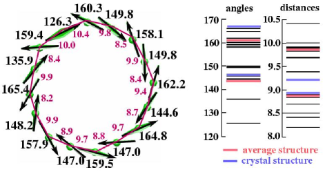
FIG. 3.: Orientation of B850 BChls resulting from a snapshot of a 10 ps long molecular dynamics simulation. Orientation of the Q_y transition dipole moments is indicated by arrows. Angles and distances between the nearest neighbors (in degrees and in Å), averaged over a 10 ps long simulation, are given on the outside and on the inside of the ring, respectively. The same numbers are shown in the right-hand side of the Figure, and compared to the angles and distances of the crystal structure.

2 B800 BChls

The crystal structure of LH-II of Rs. molischianum revealed an unusual ligation of the B800 BChls [6]. In variance with the customary ligation of BChl’s central Mg atom to a His residue (as found for the B850 BChls), the Mg atom of B800 BChls is coordinated to the O$\delta_{1}$ atom of an Asp residue. In addition, an H₂O molecule is found in the vicinity of the ligation site. The initial, minimized structure of LH-II embedded into a lipid-water environment did not contain any water molecules within the B800 binding pocket. During the course of the equilibration, a water molecule diffused into the B800 binding pocket for seven out of eight of the B800 BChls. In Fig. 4 we show a diffusion pathway of a water molecule into the binding site of one of the B800 BChls, recorded over the first 440 ps of the equilibration run. Representative distances within the binding pocket, averaged over the 10 ps long simulation, are shown in Fig. 4: 2.72 Å (O atom of H₂O to O$\delta 1$ atom of Asp6), 3.76 Å (O atom of H₂O to Mg atom of BChl), 3.16 Å (carbonyl O2 atom of BChl to O atom of H₂O), 2.00 Å (Mg atom of BChl to O$\delta 1$ atom of Asp6). The respective distances determined for the crystal structure of LH-II are 2.74 Å, 4.24 Å, 3.10 Å and 2.45 Å, respectively [6].

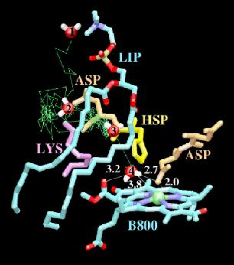
FIG. 4.: Binding pocket for B800 BChl and surrounding protein and lipid residues. Shown, in green, is a trajectory of a water molecule, obtained from a 440 ps long simulation. Snapshots of the water molecule at times t = 0 (1), t = 230 ps (2), t = 360 ps (3), t = 362 ps (4) are represented. Distances, averaged over a 10 ps simulation, of the O atom of the water molecule, in position (4), with key protein and BChl atoms are given.

B Time-series analysis of simulation data

The time series analysis presented in this section is based on an 800 fs long MD simulation. We recorded the nuclear ($R(t_{k})$) and bath ($Z(t_{k})$) coordinates every 2 fs, and generated a total of 400 snapshots. Based on $R(t_{k})$, and $Z(t_{k})$, we performed a total of 16 $\times$ 400 quantum chemistry calculations, resulting in excitation energies $\epsilon_{i}(t_{k})$, $i=1,...,16$, for each snapshot $k$. Based on $R(t_{k})$ and $Z(t_{k})$, we also calculated $W_{i,j}(t_{k})$ according to Eq. (16). Combining $\epsilon_{i}(t_{k})$ and $W_{i,j}(t_{k})$ we constructed the time-dependent exciton Hamiltonian (15).

1 Exciton Hamiltonian

Fluctuations of two representative elements of Hamiltonian matrix (15) are presented in Fig. 5. The fluctuations of the largest off-diagonal matrix elements, i.e., couplings between neighboring BChls, are two orders of magnitude smaller than the fluctuations of diagonal matrix elements. The fluctuations of couplings between non-neighboring BChls are at least another order of magnitude smaller than those of the nearest neighbors. This suggests that off-diagonal disorder is negligible compared to the diagonal disorder.

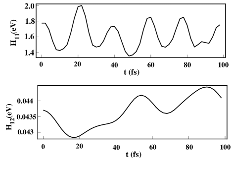
FIG. 5.: Matrix elements $H_{11}(t)=\epsilon_{1}(t)$ (top) and $H_{12}(t)=W_{12}(t)$ (bottom) of Hamiltonian (15), as calculated for the first 50 snapshots of the MD run.

Simple visual inspection of the time-dependence of $\epsilon(t)$ in Fig. 5, reveals a prominent oscillatory component of about 20 fs. Indeed, the power spectrum of $\epsilon_{i}(t)$ (averaged over all 16 BChls) defined as

$\displaystyle\sqrt{\frac{1}{16}\sum_{i=1}^{16}\left|\int_{0}^{\infty}dte^{i\omega t}\epsilon_{i}(t)\right|^{2}}\;,$

and shown in Fig. 6, displays strong components in the range between 0.2 eV and 0.22 eV, corresponding to the oscillations with a period of 20.6 fs and 19.1 fs, respectively. These modes most likely originate from a C=O or a methine bridge stretching vibration. We note that the autocorrelation function of Q_y excitation energy of BChl in methanol also displays a prominent vibrational mode of about 18 fs period [41].

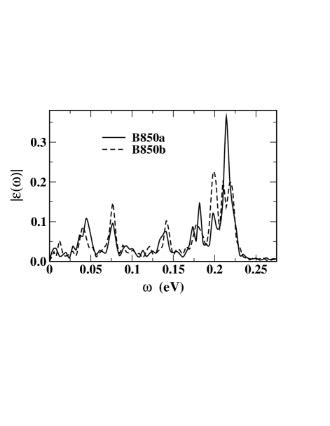
FIG. 6.: Average power spectrum of matrix elements $\epsilon_{i}(t)$, for B850a BChls $i=1,3,\ldots,15$ (full line), and for B850b BChls, $i=2,4,\ldots,16$ (dashed line).

Fig. 6 reveals further vibrational modes. While the B850a and B850b BChls have some common modes (0.198 eV, 0.141 eV, 0.077 eV), some other modes peak at slightly different energies; 0.218 eV, 0.21 eV, 0.182 eV, 0.174 eV, 0.045 eV for B850a as compared to 0.214 eV, 0.178 eV, 0.040 eV for B850b. These differences most likely stem from the difference in the protein environment seen by B850a and B850b.

A histogram of excitation energies $\epsilon_{k}(t)$ of all 16 BChls, is shown in Fig. 9. Histograms of 8 B850a BChls and 8 B850b BChls (data not shown) reveal rather large values for the full-width at half-maximum (FWHM), of about 0.21 eV for B850a and 0.25 eV for B850b. Furthermore, the lineshape in Fig. 9 reveals a non-Gaussian distribution. The same non-Gaussian distribution of excitation energies was observed in [41]. The reason for such a distribution might be strong coupling to the high-frequency modes.

The Hamiltonian (15) was diagonalized for each snapshot $t_{k}$ of the simulation, assuming that it is constant in the interval $[t_{k},\,t_{k+1}]$. Fluctuations of the excitonic energies that result from the diagonalization are shown in Fig. 7. The Figure also shows energies of the 16 excitonic states averaged over the 800 fs long run, versus a corresponding average of the dipole strength. Dipole strengths are given in units of individual BChl dipole strength (1 $S_{y}$). As can be inferred from Fig. 7, only the lowest five excitonic levels have dipole strengths larger than 1. This suggests that in a thermally disordered exciton system the spectral maximum experiences a red-shift relative to the absorption maximum of an individual BChl.

For comparison we show excitonic energies and dipole strengths for the Hamiltonian that corresponds to the perfect symmetric crystallographic structure. Energetic degeneracies of the exciton states are lifted in the fluctuating case and excitonic energies spread due to disorder. On the other hand, dipole strength, which is mostly contained in two degenerate excitonic levels in the symmetric case, is distributed more equally among the exciton states in case of the disordered system. The dipole forbidden nature of the lowest exciton state of the symmetric case is lifted in the disordered case.

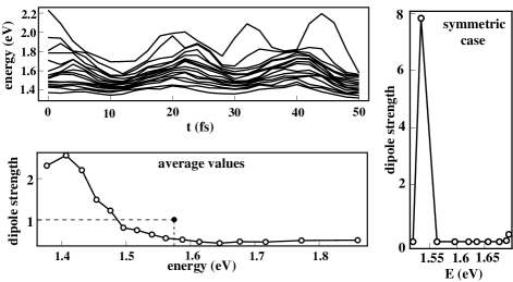
FIG. 7.: Top, left: Excitonic energies, as determined by diagonalization of Hamiltonian (15) for the first 25 snapshots of the MD simulation. Energies are in eV. Bottom, left: Average energies of the 16 excitonic levels versus their corresponding average dipole strengths. Dipole strengths are given in units of dipole strength (1 $S_{y}$) of individual BChls. The filled circle indicates the excitation energy (1.57 eV) and the unit dipole strength of an individual BChl. Right: Excitonic energies for a symmetric (see text) Hamiltonian, versus corresponding dipole strengths.

2 Absorption spectrum

The absorption coefficient $\alpha(\omega)$ of the excitonically coupled B850 BChls was calculated by employing Eqs. (19,21,64). The Hamiltonian $\hat{H}(t_{k})$ was assumed to be constant in the time interval $t_{k+1}-t_{k}=0.5$ fs, and the evolution operators $U(t_{k+1},t_{k})$ in Eq. (19) were determined accordingly. Since molecular dynamics trajectories were recorded only every 2 fs we generated additional data points for the Hamiltonian by linear interpolation. Ensemble averaging was achieved by dividing the total simulation time of 800 fs into 40 fs long time intervals, which resulted in a total of 20 samples of 40 fs length. The integrand in Eq. (64) is shown in Fig. 8. The fast fluctuation of the integrand required a choice of 0.5 fs for the time discretization. The resulting normalized spectrum is also shown in Fig. 8.

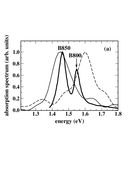
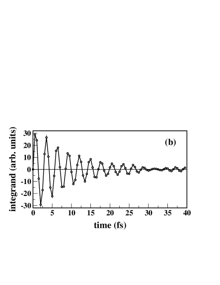
FIG. 8.: (a) Comparison of absorption spectra of B850 exciton (solid line) and individual BChls (dashed line), both obtained through Fourier transform of the time series data (see text) with the experimental absorption spectrum of B850 and B800 (solid thick line) [42]. (b) Time-dependence of the integrand in Eq. (64).

The calculated exciton absorption spectrum is compared in Fig. 8 to the experimentally measured spectrum. The calculated spectrum has a FWHM of about 0.138 eV, which is considerably larger than the FWHM of 0.05 eV for the experimental spectrum. Below we will discuss possible reasons for this discrepancy.

We have also determined the absorption spectrum of individual BChls, according to Eq. (68). The spectrum was obtained from a sample of 320 ($800\times 16/40$) MD runs of 40 fs length. The integration time-step was again 0.5 fs. The FWHM of the individual BChl absorption spectrum is about 0.125 eV, and its maximum is blue shifted with respect to the maximum of the exciton absorption spectrum. This shift is in agreement with the above mentioned transfer of dipole strength into low energy exciton states (see Fig. 7).

Our test calculations indicate that for both the individual BChl and exciton case, the additional peaks on both sides of the main absorption peak are unphysical and are most likely a consequence of insufficient sampling.

The exciton spectrum is slightly broader than the spectrum of individual BChls, apparently indicating the lack of an exchange narrowing of the absorption spectrum. Exchange narrowing is well known in J-aggregates with static disorder [43], and is caused by excitonic interactions within an aggregate, i.e., the excitation experiences more than one realization of disorder, and, thus, effective disorder is an average over those realization. For purely statically disordered LH-II aggregates, the exchange narrowing factor was found to be about 2.8 [7], in agreement with the theoretical value $\sqrt{N}$, where $N$ characterizes the N-fold symmetry of the aggregate, i.e., in the present case $N=8$. Exchange narrowing was also shown to occur for dynamically disordered aggregates. For a particular model, the authors in [44] have derived an expression for the narrowing factor which depends on the size of the aggregate, correlation time of the fluctuation $t_{c}$, as well as the strength of the excitonic coupling $J$. For the values characteristic for our simulation, $t_{c}\sim 20$ fs, and $J\sim 300$ cm^-1, the exchange narrowing factor is about unity. Thus, provided that the model of Ref. [44] is applicable to our simulation, this result may explain the absence of exchange narrowing of our exciton absorption spectrum.

3 Discussion of the results of the simulations

For about 30 $\%$ of the MD geometries the quantum chemistry calculations predicted a slight degree of mixing between the Q_y and Q_x states. If this mixing was only an artifact of quantum chemistry calculations, it would have resulted in the Q_y energy being predicted too low, and fluctuation of the excitation energy to be unrealistically large. An immediate test of the validity of the quantum chemistry calculations is provided by a comparison of the predicted mean energy gap of 0.45 eV between the Q_y and Q_x states with the corresponding experimental value. Taking into account the additional shift due to excitonic interactions in the Q_y band, of about 0.13 eV, as predicted by our calculations, it appears that the quantum chemistry calculations account correctly for the experimentally measured $0.6$ eV of the mean energy gap. More refined quantum chemistry calculations are necessary to determine if the Q${}_{y}\,-\,$Q_x mixing is indeed genuine.

Next we discuss the choice of nearest-neighbor couplings. Various estimates of these couplings have been reported in the literature; for LH-II of Rs. molischianum: 806 cm^-1 and 377 cm^-1 (semiempirical INDO/CIS calculations/effective Hamiltonian calculations [45, 7]), 408 cm^-1 and 366 cm^-1 (collective electronic oscillator approach [46]); for LH-II of Rps. sphaeroides: 300 cm^-1 and 233 cm^-1 (circular dichroism studies [47]); for LH-II of Rps. acidophila: 238 cm^-1 and 213 cm^-1 [48], 320 cm^-1 and 255 cm^-1 [49] (CIS Gaussian 94 calculations), 394 cm^-1 and 317 cm^-1 (QCFF/PI calculation [50]), 622 cm^-1 and 562 cm^-1 (ZINDO/S method [51]). The average values of couplings used in this paper are 364 cm^-1 and 305 cm^-1. If larger values were used, as might have been suggested from some of the above mentioned estimates, a narrower absorption spectrum would have been predicted, due to an increase in the exchange narrowing factor.

To reduce computational cost of our simulation, we employed the dipole-dipole approximation to describe variations of the nearest neighbor couplings as a function of time. It is well known that this approximation does not hold in the case when center-to-center distances between pigments are smaller than the size of the pigments themselves. However, we find that the fluctuations of the amplitude of off-diagonal matrix elements is negligible compared to the fluctuations of the diagonal matrix elements, and we expect that this would still hold if the proper coupling between the neighboring pigments was determined.

V Analysis in the Framework of the Polaron Model

In order to describe the influence of dynamical disorder (thermal fluctuations) on the electronic excitations of the B850 BChls, we will employ now a model that focuses on the effect of the strongest fluctuations in the exciton Hamiltonian (15), the variation of the site energies $\epsilon_{j}(t)$. These variations are foremost due to the coupling of the high-frequency vibrations to Q_y excitations in BChl (see Fig. 6). Initially, we will model this coupling through a single harmonic oscillator mode $\omega_{0}$, that is coupled to each of the local BChl excitations and, thereby, to the exciton system. Both the selected vibrational mode and the exciton system will be described quantum mechanically, replacing the time dependence of the Hamiltonian (15) by a time-independent Hamiltonian that includes the selected vibrational mode and the exciton system. We assume that the electronic excitations of the B850 BChls form a linear system of coupled two-level systems, which interact at each site with dispersionless Einstein phonons of energy $\hbar\omega_{0}$. To simplify our notation, we will assume units with $\hbar\,=\,1$. The corresponding model Hamiltonian, the so-called Holstein Hamiltonian[52], reads

$$H = H_{ex}+H_{ph}+H_{int}\;,$$ (70)

$$H_{ex} = \sum_{i}\epsilon_{i}\,B_{i}^{\dagger}\,B_{i}\,+\,\sum_{i\neq j}V_{ij}\,B_{i}^{\dagger}\,B_{j}\,,$$ (71)

$$H_{ph} = \sum_{i}\omega_{0}\,b_{i}^{\dagger}\,b_{i}\,,$$ (72)

$$H_{int} = g\,\omega_{0}\,\sum_{i}B_{i}^{\dagger}\,B_{i}\,(b_{i}^{\dagger}\,+\,b_{i})\;.$$ (73)

Here $H_{ex}$ describes the electronic excitations of BChls; $B_{i}^{\dagger}$ and $B_{i}$ are creation and annihilation operators accounting for the electronic excitation of BChl_i with excitation energy $\epsilon_{i}$; $V_{ij}$ [c.f., Eq. (16)] encompasses the coupling between excitations of BChl_i and BChl_j; $H_{ph}$ represents the selected vibrations of the BChls where $b_{i}^{\dagger}$ and $b_{i}$ denote the familiar harmonic oscillator creation and annihilation operators. $H_{int}$ describes the interaction between excitons and phonons, scaled by the dimensionless coupling constant $g$.

The stationary states corresponding to the Hamiltonian (V) are excitons “dressed” with a phonon cloud and are referred to as polarons. Accordingly, the suggested description is called the polaron model. In what follows we shall restrict ourself only to the “symmetric case”, i.e., we assume $\epsilon_{i}=\epsilon_{0}$ for all sites, and we set $V_{ij}=-V\delta_{j,i\pm 1}$, where $V$ is the nearest neighbor interaction energy. This choice of the Hamiltonian is motivated by the results of our simulations, which suggest that the exciton dynamics is determined by the size- and time-scales of the thermal fluctuations of the excitation energies, $\epsilon_{i}$, of individual BChls. Indeed, as shown in Fig. 5, the magnitude of the fluctuations of $\epsilon_{i}$ is two orders of magnitude larger than the one corresponding to the nearest neighbor coupling energies, $V_{i,i\pm 1}$, and at least three orders of magnitude larger than the one corresponding to the coupling energies between non-neighboring BChls ($V_{ij}$, with $j\neq i\pm 1$). Furthermore, according to Fig. 5, the period of oscillation of $\epsilon_{i}(t)$ ($i=1,\ldots,16$) of a single BChl is about 20 fs, which corresponds to a high frequency intramolecular vibronic mode of energy $\omega_{0}=1,670$ cm${}^{-1}=207$ meV (see also Fig. 6). In the exciton Hamiltonian we set $\epsilon_{i}=\epsilon_{0}=1.57$ eV, and $V=350.9$ cm${}^{-1}=43.5$ meV, corresponding to an exciton bandwidth of $4V=174$ meV.

The effect of static disorder can be incorporated into this model by defining $\epsilon_{i}$ and $V_{ij}$ as random variables drawn from a suitably chosen distribution, which best characterizes the nature of the disorder. In this case, in calculating different physical observables, besides the usual thermal average, a second, configuration average needs to be performed.

The stationary states of the Holstein polaron Hamiltonian (V) cannot be described analytically and one needs a suitable approximation. In general, well controlled perturbative approximations are available only in the weak ($g\ll 1$; for a more precise criteria see below) and strong ($g\gg 1$) coupling limits. Besides conventional perturbation theory, the cumulant expansion method provides a convenient alternative for solving the polaron problem. The advantage of this method is that it provides reliable results even for arbitrary values of the coupling constant $g$ [53]. By using our computer simulation results, we will estimate the value of $g$ and show that our system falls into the weak exciton-phonon coupling regime. Then, we will use both perturbation theory and the cumulant expansion method to investigate within the framework of the polaron model the effect of thermal fluctuations on the exciton bandwidth, coherence size, and absorption line-shape.

A Evaluation of coupling constant g

The coupling constant $g$ can be evaluated by estimating the effect of thermal fluctuations on the electronic excitations of individual BChls. This corresponds to setting $V_{ij}\,=\,0$ in (V). In fact, in calculating excitation energies $\epsilon_{i}(t)$ in our simulations we had not accounted for excitonic coupling. As a result, we can use $\epsilon_{i}(t)$, $i=1,\ldots,M$ obtained from the simulations, to calculate the corresponding distribution function histogram [or density of state (DOS)] $\rho(\epsilon)=dN(\epsilon)/d\epsilon$ (see Fig. 9), as well as, any of the corresponding moments $\langle\epsilon^{n}_{i}\rangle=(1/N)\sum_{j=1}^{N}\epsilon_{i}^{n}(t_{j})$. The coupling constant $g$ can be determined by fitting to these data the prediction from Hamiltonian (V), for $V_{ij}\,=\,0$. The statistics for $\rho(\epsilon)$ can be improved by averaging over all sixteen B850 BChls. Since we assume that all sites are equivalent, we can restrict ourself to the model Hamiltonian

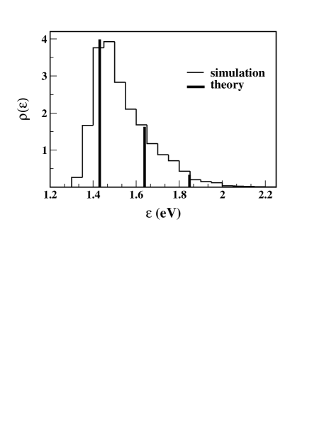
FIG. 9.: Histogram of the fluctuations $\rho(\epsilon)$ of individual BChl excitation energies $\epsilon_{i}$ obtained from quantum chemistry calculations. The vertical bars represent the weights of the Dirac-delta functions in the corresponding analytical result (V A).

$${\cal H}\;=\;\epsilon_{0}B^{\dagger}B+\omega_{0}b^{\dagger}b+g\omega_{0}B^{\dagger}B(b+b^{\dagger})\;,$$ (74)

where, for brevity, we dropped the irrelevant “i” site index.

The DOS $\rho(\epsilon)$ can be obtained from the imaginary part of the Fourier transform of the retarded Green’s function $G_{R}(t)=-i\Theta(t)\langle B(t)B^{\dagger}(0)\rangle$ [53], where $\langle\ldots\rangle$ denotes the thermodynamic average over the vibrational (phonon) degrees of freedom in the exciton vacuum. Accordingly, we employ the identity

$$\rho(\epsilon)\;=\;-\frac{1}{\pi}{\rm Im}G_{R}(\epsilon)\;,$$ (75)

where

$$G_{R}(\epsilon)=\int_{-\infty}^{\infty}dt\,G_{R}(t)e^{i\epsilon t}\;.$$ (76)

It should be noted that, because we are dealing with a single exciton coupled to a phonon bath, (i) the retarded Green’s function will coincide with the real time Green’s function $G_{R}(t)=G(t)=-i\langle TB(t)B^{\dagger}(0)\rangle$ (here $T$ denotes the time ordering operator), and (ii) the exciton-phonon coupling will not alter the phonon Green’s function. The latter can be written as [53]

$$D(t)=-i\langle TA(t)A(0)\rangle = -i[(N_{0}+1)\exp(-i\omega_{0}|t|)$$ (78)

$$+N_{0}\exp(i\omega_{0}|t|)]\;,$$

where

$$A(t)=b\exp(-i\omega_{0}t)+b^{\dagger}\exp(i\omega_{0}t)$$ (79)

is the phonon field operator, $N_{0}=1/[\exp(\beta\omega_{0})-1]$ is the Bose-Einstein distribution function, and $\beta=1/k_{B}T$. At room temperature ($T\approx 300$ K), we have $\beta\omega_{0}\approx 8.1$, and consequently $N_{0}\approx 3.1\times 10^{-4}\ll 1$. Thus, as we have already mentioned, the thermal population of the high frequency vibrational mode $\omega_{0}$ is negligibly small even at room temperature.

In order to calculate the Green’s function we separate the Hamiltonian (74) into two contributions ${\cal H}={\cal H}_{0}+{\cal H}_{int}$, where ${\cal H}_{0}$ accounts for the first term in (74). Accordingly, we express

$$G(t)=-i\langle TB(t)B^{\dagger}(0)\rangle=G_{0}(t)\exp[-\Phi(t)]\;,$$ (80)

where

$$G_{0}(t)=-i\Theta(t)\exp(-i\epsilon_{0}t)$$ (81)

is the Green’s function corresponding to ${\cal H}_{0}$. We then employ the cumulant expansion method [53] writing

$$G_{0}(t)\exp[-\Phi(t)]\equiv G_{0}(t)\exp\left[-\sum_{m=1}^{\infty}\Phi_{m}(t)\right]=\sum_{m=0}^{\infty}W_{m}(t)\;,$$ (82)

where

$$W_{m}(t) = \frac{(-i)^{2m}}{(2m)!}\int_{0}^{t}dt_{1}\ldots\int_{0}^{t}dt_{2m}$$ (84)

$$\times\langle TB(t){\cal H}_{int}(t_{1})\ldots{\cal H}_{int}(t_{2m})B^{\dagger}(0)\rangle\;,$$

and ${\cal H}_{int}(t)=g\omega_{0}B^{\dagger}BA(t)$. The cumulants $\Phi_{m}$ are expressed in terms of $W_{m}$ by identifying on both sides of Eq. (82) all the terms which contain the same power of $H_{int}$. By using Eqs. (84,78) we have

$$W_{1}(t) = -(g\omega_{0})^{2}G_{0}(t)\int_{0}^{t}dt_{1}\int_{0}^{t_{1}}dt_{2}D(t_{1}-t_{2})$$ (85)

$$= G_{0}(t)[i\epsilon_{p}t-S_{0}+S_{+}\exp(-i\omega_{0}t)+S_{-}\exp(i\omega_{0}t)]\;,$$ (86)

where

$$\epsilon_{p}=g^{2}\omega_{0}$$ (87)

is the polaron binding energy, and

$$S_{0}=g^{2}(2N_{0}+1)\;,\qquad S_{\pm}=g^{2}(N_{0}+1/2\pm 1/2)\;.$$ (88)

From these results follows

$$\Phi_{1}(t)=-G_{0}^{-1}(t)W_{1}(t) = -i\epsilon_{p}t+S_{0}-S_{+}\exp(-i\omega_{0}t)$$ (90)

$$-S_{-}\exp(i\omega_{0}t)\;.$$

By employing Wick’s theorem[53], one can calculate $W_{m}$, for arbitrary integer $m>1$, with the result $W_{m}=G_{0}[G_{0}^{-1}W_{1}]^{m}/m!$. Consequently, we find $\Phi_{m}(t)=0$ for $m>1$. The exact exciton Green’s function is then given by

$$G(t) = -i\Theta(t)\exp[-i(\epsilon_{0}-\epsilon_{p})t-\Phi_{0}(t)]\;,$$ (92)

$$\Phi_{0}(t) = S_{0}-S_{+}\exp(-i\omega_{0}t)-S_{-}\exp(i\omega_{0}t)\;.$$ (93)

In order to calculate the DOS, we express Eq. (93) in the equivalent form

$$\Phi_{0}(t) = e^{-g^{2}(2N_{0}+1)}\exp\{2g^{2}\sqrt{N_{0}(N_{0}+1)}$$ (95)

$$\times\cos[i\omega_{0}(t+i\beta/2)]\}\;,$$

and employ the identity

$$e^{z\cos\theta}=\sum_{\ell=-\infty}^{\infty}{\rm I}_{\ell}(z)\,e^{i\ell\theta}\;,$$ (96)

where ${\rm I}_{\ell}(z)$ is the modified Bessel function. From Eqs. (75,V A-96) one obtains finally the well known result [53, 54]

$$\rho(\epsilon)=\sum_{\ell=-\infty}^{\infty}\rho_{\ell}\,\delta(\epsilon-\epsilon_{\ell})\;,$$ (98)

with

$$\rho_{\ell}=\exp[-g^{2}(2N_{0}+1)+\ell(\beta\omega_{0}/2)]\;{\rm I}_{\ell}(2g^{2}\sqrt{N_{0}(N_{0}+1)})\;,$$ (99)

and

$$\epsilon_{\ell}=\omega_{0}\ell+\epsilon_{0}-\epsilon_{p}\;.$$ (100)

In general, when the coupling $V_{ij}$ between excitons cannot be neglected, the higher order cumulants $\Phi_{m}$ do not vanish, and the Green’s function $G(t)$ cannot be calculated exactly. Nevertheless, even in this case, the cumulant expansion method, as illustrated above in deriving the well known result (V A), can be conveniently applied to calculate perturbatively, in a systematic way, both the Green’s function and the corresponding absorption spectrum (see below) to any desired degree of accuracy.

The calculated DOS (normalized to unity) is an infinite sum of Dirac-delta functions at energies $\epsilon_{\ell}$, with weights $\rho_{\ell}$. As shown in Fig. 9, for a proper choice of the exciton-phonon coupling constant $g$, the “stick-DOS” (i.e., the weights $\rho_{\ell}$) matches well the histogram $\rho(\epsilon)$ obtained from our quantum chemistry calculations. The coupling constant $g$ was determined by matching the first few moments of $\epsilon$, once calculated according to Eqs. (98-100), and then from the time series $\{\epsilon_{i}(t)\}_{i=1,...,16}$. The definition of the moments

$$\langle\epsilon^{n}\rangle=\int_{-\infty}^{\infty}d\epsilon\rho(\epsilon)\epsilon^{n}=\sum_{\ell}\rho_{\ell}\epsilon_{\ell}^{n}\;,$$ (101)

applied to (98-100), results in analytical expressions that can be compared with the numerical values determined from the time series. One obtains

$$\langle\epsilon\rangle = \epsilon_{0}\approx 1.57~{}{\rm eV}\;,$$ (103)

$$\langle\epsilon^{2}\rangle = \langle\epsilon\rangle^{2}+g^{2}(2N_{0}+1)\omega_{0}\approx 2.32~{}{\rm eV}^{2}\;,$$ (104)

$$\langle\epsilon^{3}\rangle = \langle\epsilon\rangle^{3}+g^{2}\omega_{0}^{3}\left[1+3g^{2}(2N_{0}+1)\right.$$ (106)

$$\left.+3(2N_{0}+1)\left(\frac{\epsilon_{0}}{\omega_{0}}-g^{2}\right)\right]\approx 3.56~{}{\rm eV}^{3}\;.$$

The coupling constant can be obtained from Eq. (104)

$$g=\sqrt{\frac{\langle\epsilon^{2}\rangle-\langle\epsilon\rangle^{2}}{(2N_{0}+1)\omega_{0}^{2}}}\approx 0.65\;,$$ (107)

Equation (106) now contains no adjustable parameters and it can be used to check the reliability of our approach. It is found that the difference between the two sides of this equation is less than $2\%$.

The value of $g$, given by (107), does not determine by itself the value of the ratio between $H_{int}$ ($\sim\epsilon_{p}$) and the problematic hopping term ($\sim 4V$, i.e., the energy bandwidth of the excitons) in the Holstein Hamiltonian. The actual dimensionless coupling strength parameter for the polaron model is $\kappa\equiv\epsilon_{p}/4V=g^{2}\omega_{0}/4V\approx 0.5$. This value corresponds to a weak coupling regime of the polaron model [53, 54].

B Polaron bandwidth

We return now to the full Holstein Hamiltonian (V) with $V_{ij}\,\neq\,0$. In the weak coupling limit it is convenient to rewrite the polaron Hamiltonian (V) in “momentum space” as

$$H = H_{0}+H_{int}\;,$$ (109)

$$H_{0} = \sum_{k}\epsilon_{k}B^{\dagger}_{k}B_{k}+\omega_{0}\sum_{q}b^{\dagger}_{q}b_{q}\;,$$ (110)

$$H_{int} = \frac{g\omega_{0}}{\sqrt{M}}\sum_{k,q}B^{\dagger}_{k+q}B_{k}(b^{\dagger}_{q}+b_{-q})\;,$$ (111)

where $B_{k}=(1/\sqrt{M})\sum_{j}B_{j}\exp(ikj)$, etc. For $V_{ij}=-V\delta_{j,i\pm 1}$ ($V>0$), the exciton dispersion (measured from the site excitation energy $\epsilon_{0}$) is $\epsilon_{k}=-2V\cos(k)$, with $k\equiv k_{m}=2\pi m/M$, $m=0,1,\ldots,M-1$, and $q\equiv q_{p}=2\pi p/M$, $p=0,1,\ldots,M-1$.

The polaron (phonon renormalized exciton) spectrum $E_{k}$ can be calculated by using second order perturbation theory (all odd order terms vanish because the phonon creation and annihilation operators must appear in pairs)

$$E_{k}=\epsilon_{k}+\frac{g^{2}\omega_{0}^{2}}{M}\sum_{q}\frac{1}{\epsilon_{k}-\epsilon_{k+q}-\omega_{0}}\;.$$ (112)

The renormalized exciton wave functions to leading order in $g$ are given by

$$|k;0)=|k;0\rangle+\frac{g\omega_{0}}{\sqrt{M}}\sum_{q}\frac{1}{\epsilon_{k}-\epsilon_{k+q}-\omega_{0}}|k+q;1_{q}\rangle\;.$$ (113)

Here $|k;0\rangle=(1/\sqrt{M})\sum_{m}\exp(ikm)|m\rangle$ denotes the exciton wave function (in site $|m\rangle$ representation) in the absence of the phonons, while $|k+q;1_{q}\rangle$ represents a state of non-interacting exciton (with momentum $k+q$) and phonon (with momentum $q$). The applicability of perturbation theory is subject to the condition $g\omega_{0}/\sqrt{M}\ll|\epsilon_{k}-\epsilon_{k+q}-\omega_{0}|$, which in our case is marginally fulfilled since $g\omega_{0}/\sqrt{M}=33$ meV$<\text{min}|\epsilon_{k}-\epsilon_{k+q}-\omega_{0}|=35$ meV.

According to Eq. (112) the renormalized exciton (or polaron) bandwidth is

$$\Delta E_{p}\equiv\text{max}[E_{k}]-\text{min}[E_{k}]\approx 66\text{meV}\;,$$ (114)

which represents a $60$% reduction with respect to the unperturbed bandwidth $4V$. Thus the effect of the high frequency phonons is to reduce the exciton energy band, a situation commonly encountered in other weak coupling polaron models in which the phonons tend to enhance the quasiparticle mass, which is translated into a reduction of the width of the corresponding energy band [53, 54]. However, it is known that static disorder (or coupling to low frequency phonons) has precisely the opposite effect of increasing the exciton bandwidth in BChl aggregates. The fact that in our MD simulations we observe an increase instead of a decrease of the renormalized exciton bandwidth is most likely due to the fact that in our simplified polaron model the effect of static disorder is entirely neglected, while in the MD simulations this is implicitly included.

C Polaron coherence length

Next, we determine the effect of the phonons on the coherence length $L_{\rho}$ of the excitons in the BChl ring, by using our polaron model. At zero temperature, the excitons in the coupled BChl aggregate are completely delocalized, and $L_{\rho}$ should coincide with the system size $M$. In general, finite temperature and any kind of disorder will reduce the coherence length of the exciton. There is no universally accepted definition of $L_{\rho}$. We employ here an expression based on the concept of inverse participation ratio, familiar from quantum localization [55, 13]

$$L_{\rho}=\left[\left(\sum_{ij}|\rho_{ij}|\right)^{2}\right]\left[M\sum_{ij}|\rho_{ij}|^{2}\right]^{-1}\;,$$ (115)

where the reduced exciton density matrix is given by

$$\rho_{ij}=\sum_{k}C_{k}^{*}(i)C_{k}(j)\exp(-\beta E_{k})\;.$$ (116)

In the absence of the exciton-phonon coupling, at room temperature, by setting in the above equations $C_{k}(j)=\exp(ikj)/\sqrt{M}$ and $E_{k}\equiv\epsilon_{k}=-2V\cos(k)$, one obtains $L_{\rho 0}\approx 6.4$, which represents a dramatic decrease with respect to the corresponding zero temperature value of 16. For weak exciton-phonon coupling, the effect of the phonons on $L_{\rho}$ can be taken into account via perturbation theory. By employing Eqs. (112,113) in the density matrix (116), Eq. (115) yields $L_{\rho}\approx 5.4$. As expected, the phonons, which act as scatterers for the excitons, reduce the coherence size of the latter.

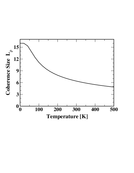
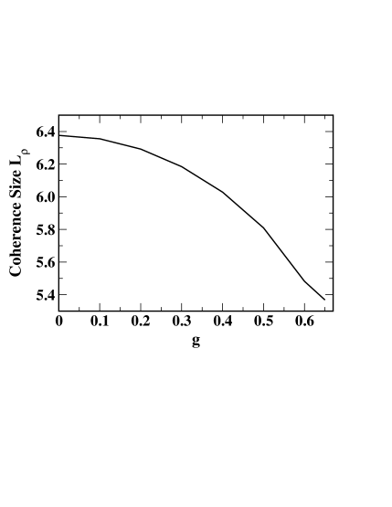
FIG. 10.: Top: Temperature dependence of the exciton coherence length in the absence of disorder. Bottom: Polaron coherence length as a function of the exciton-phonon coupling constant $g$ at room temperature.

As it can be inferred from Fig. 10, the localization of the exciton is due primarily to thermal averaging and to a lesser extent to dynamic disorder. This conclusion is in agreement with previous studies [14].

D Absorption spectrum for single Einstein phonon

Finally, we discuss the effect of the phonons on the absorption spectrum of the excitons. The fundamental absorption spectrum $I(\omega)$ (line shape function) is defined as [cf. Eq. (68)]

$$I(\omega)=\frac{1}{2\pi}\int_{-\infty}^{\infty}dtf(t)e^{i\omega t}\;,$$ (117)

where the generating function $f(t)$, up to irrelevant factors, is given by [54]

$$f(t)=\sum_{k}|d_{k}|^{2}e^{-i\epsilon_{k}t}\langle\langle k|U(t)|k\rangle\rangle\;.$$ (118)

Here $|d_{k}|$ is the magnitude of the transition dipole moment connecting the ground electronic state and the $|k\rangle$ exciton state; $\langle\langle k|\ldots|k\rangle\rangle$ denotes the thermal average over the phonons of the excitonic matrix element $\langle k|\ldots|k\rangle$, and $U(t)$ is an evolution operator given by

$$U(t) = \exp(iH_{0}t)\exp[-i(H_{0}+H_{int})t]$$ (119)

$$= T\exp\left[-i\int_{0}^{t}d\tau H_{int}(\tau)\right]\;,$$ (120)

with

$$H_{int}(t) = \exp(iH_{0}t)H_{int}\exp(-iH_{0}t)$$ (122)

$$= g\omega_{0}\sum_{q}\rho_{q}(t)A_{q}(t)\;,$$ (123)

expressed in the interaction representation. The time dependent exciton density operator is given by

$$\rho_{q}(t)=\sum_{k}e^{-i(\epsilon_{k}-\epsilon_{k+q})t}B_{k+q}^{\dagger}B_{k}\;,$$ (124)

while the phonon field operator reads

$$A_{q}(t)=b_{q}e^{-i\omega_{0}t}+b_{-q}^{\dagger}e^{i\omega_{0}t}\;.$$ (125)

The generating function (118) can be calculated by using the cumulant expansion method discussed above. Indeed, we can write in analogy to Eqs. (82,84)

$$\langle\langle k|U(t)|k\rangle\rangle\equiv\exp[-\Phi_{k}(t)] = \exp\left[-\sum_{m=1}^{\infty}\Phi_{m}(t)\right]$$ (126)

$$= \sum_{m=0}^{\infty}W_{m}(t)\;,$$ (127)

where

$$W_{m}(t)=\frac{(-i)^{2m}}{(2m)!} \int_{0}^{t}dt_{1}\ldots\int_{0}^{t}dt_{2m}$$ (129)

$$\times\langle\langle k|TH_{int}(t_{1})\ldots H_{int}(t_{2m})|k\rangle\rangle\;.$$

As for the Green’s function (82), $W_{m}(t)$ contains only even numbers of time ordered $H_{int}(t)\propto A(t)$ operators, because the average over odd numbers of phonon field operators $A(t)$ vanishes. Similarly to Eq. (85), we have

$$W_{1}(t) = -\frac{(g\omega_{0})^{2}}{2M}\int_{0}^{t}dt_{1}\int_{0}^{t}dt_{2}\sum_{q_{1},q_{2}}\langle TA_{q_{1}}(t_{1})A_{q_{2}}(t_{2})\rangle$$ (131)

$$\times\langle k|\rho_{q_{1}}(t_{1})\rho_{q_{2}}(t_{2})|k\rangle$$

$$= -\frac{(g\omega_{0})^{2}}{2M}\int_{0}^{t}dt_{1}\int_{0}^{t}dt_{2}\sum_{q}iD(t_{1}-t_{2})$$ (133)

$$\times\langle k|\rho_{q}(t_{1})\rho_{-q}(t_{2})|k\rangle\;.$$

A straightforward calculation yields

$$F_{k}(t_{1}-t_{2}) \equiv \frac{1}{M}\sum_{q}\langle k|\rho_{q}(t_{1})\rho_{-q}(t_{2})|k\rangle$$ (134)

$$= \frac{1}{M}\sum_{q}\exp[i(\epsilon_{k}-\epsilon_{k-q})(t_{1}-t_{2})]\;.$$ (135)

Inserting Eq. (134) into (131), and using the phonon Green’s function (78), the cumulant $\Phi_{1}(t)$ can be written

$$\Phi_{1}(t)=-W_{1}(t)=g^{2}\omega_{0}^{2}\int_{0}^{t}d\tau(t-\tau)iD(\tau)F_{k}(\tau)\;.$$ (136)

If one neglects the coupling between the individual excitations (case corresponding to light absorption by individual BChls), by setting $V=0$, Eq. (136) yields the same expression as (90). Note that in this case, since $\epsilon_{k}=\epsilon_{0}$ is $k$ independent, we have $F(\tau)=1$, and similarly to the calculation of the Green’s function (V A), it can be shown that $W_{m}(t)=[W_{1}(t)]^{m}/m!$, for $m>2$. As a result, all the corresponding higher order cumulants $\Phi_{m}$ vanish, i.e., $\Phi(t)=\Phi_{1}(t)$, and the exact expression of the line-shape function $I_{0}(\omega)$ for individual BChls assumes the familiar form [53, 54]

$$I_{0}(\omega) \propto \exp(-S_{0})\int_{-\infty}^{\infty}dte^{i(\omega-\epsilon_{0}+\epsilon_{p})t}$$ (139)

$$\times\exp(-S_{+}e^{-i\omega_{0}t}-S_{-}e^{i\omega_{0}t})$$

$$= \sum_{\ell=-\infty}^{\infty}\rho_{\ell}\delta(\omega-\omega_{\ell})\;,$$ (140)

where $\rho_{\ell}$ and $\omega_{\ell}$ are given by Eqs. (99), and (100), respectively. In other words, the absorption line-shape function of an exciton in the phonon field is given by the imaginary part of the exciton Green’s function, which is proportional to the density of states [54].

In general, $I(\omega)$ cannot be calculated exactly. However, even for arbitrary values of the exciton-phonon coupling constant $g$, the cumulant approximation $\Phi_{k}(t)\approx\Phi_{1}(t)$ can be used safely to evaluate the generating function $f(t)$ and the corresponding line shape function $I(\omega)$. We have

$$\Phi_{k}(t)\approx\int_{0}^{t}d\tau(t-\tau){\cal D}(\tau)F_{k}(\tau)\;,$$ (141)

where, according to Eq. (78),

$${\cal D}(t) \equiv g^{2}\omega_{0}^{2}iD(t)$$ (142)

$$= g^{2}\omega_{0}^{2}[(N_{0}+1)e^{-i\omega_{0}t}+N_{0}e^{i\omega_{0}t}]\;.$$ (143)

The generating function is

$$f(t)=\sum_{k}|d_{k}|^{2}e^{-i\epsilon_{k}t}e^{-\Phi_{k}(t)}\;,$$ (144)

and the corresponding line shape function is given by Eq. (117). Clearly, the coupling of the 16 exciton levels to a single Einstein phonon $\omega_{0}$ leads to a stick absorption spectrum, i.e., a series of Dirac delta functions with different weights.

E Absorption spectrum for distribution of phonons

In order to calculate, in the framework of the polaron model, the broadening of the absorption spectrum, and to compare it with the corresponding experimental result [see Fig. 8], one needs to include the coupling of the excitons to the quasi-continuous distribution of the rest of the phonons. Formally, this can be achieved by replacing ${\cal D}(t)$ in Eq. (141) with [cf. Eq. (142)]

$${\cal D}(t)=\sum_{\alpha}g^{2}_{\alpha}\omega^{2}_{\alpha}iD_{\alpha}(t)=\int_{0}^{\infty}d\omega J(\omega)\,iD_{\omega}(t)\;,$$ (145)

where

$$iD_{\omega}(t)=(N_{\omega}+1)\exp(-i\omega t)+N_{\omega}\exp(i\omega t)\;.$$ (146)

Here we have introduced the phonon spectral function

$$J(\omega)=\sum_{\alpha}g^{2}_{\alpha}\omega^{2}_{\alpha}\delta(\omega-\omega_{\alpha})\;.$$ (147)

Once the actual form of $J(\omega)$ is known, $I(\omega)$ can be calculated using Eqs. (117,144,141,145).

Apparently, the determination of $J(\omega)$ requires the seemingly unattainable knowledge of the energies $\omega_{\alpha}$ of all phonons, together with their corresponding coupling constants $g_{\alpha}$. However, the same problem posed itself in the framework of the spin-boson model description of the coupling between protein motion and electron transfer processes [56], and could be solved then through a spectral function evaluated from the energy gap fluctuations $\delta{\epsilon}(t)$. Likewise, here we can determine $J(\omega)$ from the fluctuations of the excitation energies $\delta{\epsilon}(t)$ calculated for individual BChls. The latter quantity can be obtained from the combined MD/quantum chemistry simulation carried out in this study.

Indeed, the Hamiltonian for an individual BChl interacting with a phonon bath can be written

$$H=H_{0}+H_{int}=(\epsilon_{0}+\delta\hat{\epsilon})B^{\dagger}B\;,$$ (148)

where we defined the phonon induced energy-gap-fluctuation operator

$$\delta\hat{\epsilon}(t)=\sum_{\alpha}g_{\alpha}\omega_{\alpha}A_{\alpha}(t)\;.$$ (149)

The autocorrelation function of the energy gap $\delta\epsilon(t)$ is the real part of the autocorrelation function of the energy-gap-fluctuation operator $\delta\hat{\epsilon}(t)$, i.e.,

$${\cal C}(t) \equiv \langle\delta\epsilon(t)\delta\epsilon(0)\rangle=\text{Re}[\langle\delta\hat{\epsilon}(t)\delta\hat{\epsilon}(0)\rangle]$$ (150)

$$= \text{Re}\left[\sum_{\alpha}g^{2}_{\alpha}\omega^{2}_{\alpha}\,iD_{\alpha}(t)\right]=\text{Re}[{\cal D}(t)]\;,$$ (151)

where we have used Eqs. (149) and (145). Inserting Eq. (146) into (150), one obtains

$${\cal C}(t)=\int_{0}^{\infty}d\omega J(\omega)\coth(\beta\omega/2)\cos\omega t\;.$$ (152)

$J(\omega)$ can be obtained through the inverse cosine transform of ${\cal C}(t)$, i.e.,

$$J(\omega)=\frac{2}{\pi}\tanh(\beta\omega/2)\int_{0}^{\infty}\!dt\,{\cal C}(t)\,\cos\omega t\;.$$ (153)

The autocorrelation function ${\cal C}(t)$ can be evaluated numerically from the finite time series $\delta\epsilon_{j}(t_{i})$. Here $j=1,\ldots,16$ is the index labeling individual BChls, and $t_{i}=(i-1)\times 2$ fs, $i=1,\ldots,400$, denotes the time at which the energy gap was determined. As mentioned in the previous sections, each time series consisted of $N=400$ time steps of 2 fs. For best sampling, one averages over all $M=16$ BChls resulting in the time series

$${\cal C}(t_{i})=\frac{1}{M}\sum_{j=1}^{M}\left[\frac{1}{N-i}\sum_{k=1}^{N-i}\delta\epsilon_{j}(t_{i}+t_{k})\delta\epsilon_{j}(t_{k})\right]\;,$$ (154)

which is shown in Fig. 11a. It is safe to assume that Eq. (154) is reliable for $t\lesssim 400$ fs. We note that the autocorrelation function in Fig. 11a, resembles the transition frequency autocorrelation function for Nile Blue [57], obtained through a model that combines in both the intramolecular vibrations and solvent dependent contributions.

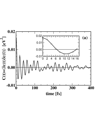
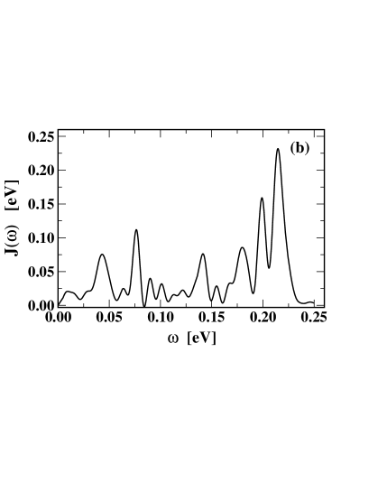
FIG. 11.: (a) Autocorrelation function ${\cal C}(t)$ of the energy gap fluctuations $\delta\epsilon(t)$ for individual BChls, calculated using Eq. (154). The inset shows the short time behavior of ${\cal C}(t)$. (b) Phonon spectral function $J(\omega)$ obtained according to Eq. (153).

The corresponding phonon spectral function $J(\omega)$ can be computed by employing Eq. (153). The result is shown in Fig. 11b. The shape of $J(\omega)$ resembles the power spectrum of the BChl excitation energies (see Fig. 6). In particular, the prominent peak around $\omega_{0}\approx 0.2$ eV in $J(\omega)$ indicates a strong coupling of the system to an intramolecular C=O vibronic mode. Note, however, that $J(\omega)$ has significant contributions over the entire range of phonon energies $0<\omega\lesssim 0.22$ eV and, therefore, we expect that all, i.e., low, intermediate and high frequency phonons will contribute to the broadening of the line shape function $I(\omega)$.

By assuming that the coupling of BChl molecules to phonons (intramolecular vibrations, vibrations of the protein matrix and solvent molecules) is independent of their excitonic coupling, we may conclude that $J(\omega)$ given by Eq. (153), describes equally well both individual BChls and excitonic aggregates of BChls. The only difference between the corresponding absorption spectra comes from the “excitonic” factor $F_{k}(t)$ in Eq. (141).

In order to calculate the line shape function $I(\omega)$, as given by Eqs. (117,141,144), from the energy gap autocorrelation function ${\cal C}(t)$ one proceeds as follows. First, we determine

$${\cal D}(t) \equiv {\cal D}_{1}(t)-i{\cal D}_{2}(t)$$ (155)

$$= \int_{0}^{\infty}d\omega J(\omega)[\coth(\beta\omega/2)\cos\omega t-i\sin\omega t]\;,$$ (156)

from which, by taking into account Eqs. (152) and (153), one obtains

$${\cal D}_{1}(t)={\cal C}(t)\;,$$ (158)

and

$${\cal D}_{2}(t)=\int_{0}^{\infty}d\omega J(\omega)\sin\omega t\;.$$ (159)

Next, we calculate the cumulant $\Phi_{k}(t)$; according to Eq. (141)

$$\Phi_{k}(t)={\Phi^{\prime}}_{k}(t)-i{\Phi^{\prime\prime}}_{k}(t)\;,$$ (161)

with

$${\Phi^{\prime}}_{k}(t)=\int_{0}^{\infty}d\tau(t-\tau)[{\cal C}(\tau)\text{Re}\{F_{k}(t)\}-{\cal D}_{2}(\tau)\text{Im}\{F_{k}(t)\}]\;,$$ (162)

and

$${\Phi^{\prime\prime}}_{k}(t)=\int_{0}^{\infty}d\tau(t-\tau)[{\cal D}_{2}(\tau)\text{Re}\{F_{k}(\tau)\}+{\cal C}(\tau)\text{Im}\{F_{k}(\tau)\}]\;.$$ (163)

Finally, the line shape function is according to Eqs. (117,144)

$$I(\omega)\propto\sum_{k}|d_{k}|^{2}\int_{0}^{\infty}dt\exp[-{\Phi^{\prime}}_{k}(t)]\cos[(\omega-\epsilon_{k})t+{\Phi^{\prime\prime}}_{k}(t)]\;.$$ (165)

This result applies to the general case when the system has several optically active levels, characterized by different transition dipole moments $d_{k}$. In both cases considered by us, i.e., individual BChls and the fully symmetric B850 system (i.e., a circular aggregate of 16 BChls with excitonic coupling, having 8-fold symmetry, and transition dipole moments oriented in the plane of the ring of BChls), there is in fact only one optically active level and, therefore, in Eq. (165) the summation over $k$, as well as the transition dipole moment can be both dropped. For an individual BChl we take $\epsilon_{k}\equiv\epsilon_{0}\approx 1.6$ eV, while for the B850 system the optically active doubly degenerate level is $\epsilon_{k}\equiv\epsilon_{\pm 1}=\epsilon_{0}-2V\cos(\pi/8)=1.52$ eV. In this case, the line shape function assumes the simpler form

$$I(\omega)\propto\int_{0}^{\infty}dt\exp[-{\Phi^{\prime}}_{k}(t)]\cos[(\omega-\epsilon_{k})t+{\Phi^{\prime\prime}}_{k}(t)]\;.$$ (166)

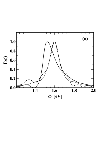
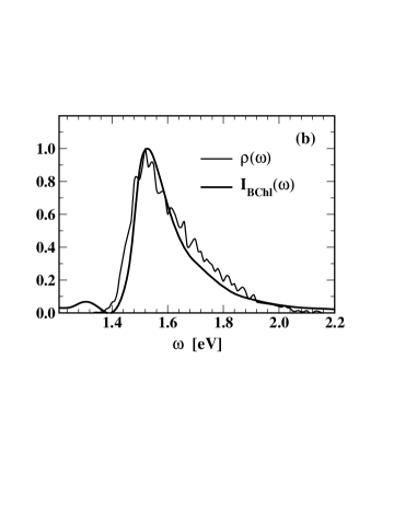
FIG. 12.: (a) Absorption spectra of individual BChls: $I(\omega)$ – time series analysis (dashed curve), $I_{0}(\omega)$ – polaron model with ${\Phi^{\prime\prime}}_{0}=0$ (thin solid curve), $I_{BChl}(\omega)$ – polaron model (thick solid curve). (b) Comparison between the normalized DOS $\rho(\omega)$ and $I_{BChl}(\omega)$, obtained within the framework of the polaron model.

In case of individual BChls, i.e., without excitonic coupling, $F_{k}(t)=1$, and according to Eqs. (166,162,163) the absorption spectrum reads

$$I_{BChl}(\omega)\propto\int_{0}^{\infty}dt\exp[-{\Phi^{\prime}}_{0}(t)]\cos[(\omega-\epsilon_{0})t+{\Phi^{\prime\prime}}_{0}(t)]\;,$$ (168)

where

$${\Phi^{\prime}}_{0}(t)=\int_{0}^{\infty}d\tau(t-\tau){\cal C}(\tau)\;,$$ (169)

and

$${\Phi^{\prime\prime}}_{0}(t)=\int_{0}^{\infty}d\tau(t-\tau){\cal D}_{2}(\tau)\;.$$ (170)

For the moment let us neglect the imaginary part of the cumulant $\Phi_{0}(t)$ in Eq. (168), i.e., we set ${\Phi^{\prime\prime}}_{0}(t)\approx 0$. It follows

$$I_{BChl}(\omega)\approx I_{0}(\omega)\propto\int_{0}^{\infty}dt\exp[-{\Phi^{\prime}}_{0}(t)]\cos[(\omega-\epsilon_{0})t]\;,$$ (171)

and one can easily see that $I_{0}(\omega)$ coincides (up to an irrelevant normalization factor) with the cumulant approximation of the line shape function $I(\omega)$, Eq. (68), derived and employed in our computer simulation study. Therefore, it comes to no surprise that in Fig. 12a the plots of the normalized [with max$\{I(\omega)\}=1$] line shape functions $I_{0}(\omega)$ and $I(\omega)$ completely overlap in the peak region. The difference between the curves away from the central peak is most likely due to poor statistics and numerical artifacts introduced by the FFT evaluation of the integrals for the time series analysis result (68). The peak of the absorption spectrum is located at $\epsilon_{0}=1.6$ eV and the corresponding FWHM is 125 meV.

However, the actual line shape function $I_{BChl}(\omega)$, as given by Eq. (168), include a non-vanishing ${\Phi^{\prime\prime}}_{0}(t)$. The corresponding result is also plotted in Fig. 12a. As one can see, the contribution of ${\Phi^{\prime\prime}}_{0}(t)$ redshifts the peak of $I_{BChl}(\omega)$ to 1.53 eV, and renders $I_{BChl}(\omega)$ asymmetric with a somewhat larger FWHM of 154 meV. As illustrated in Fig. 12b, $I_{BChl}(\omega)$ matches the corresponding DOS $\rho(\omega)$ [see Eq. (98) and Fig. 9]. This is not surprising since, as we have already mentioned, for a two level system which is linearly coupled to a phonon bath, both the DOS and the absorption spectrum are proportional to the imaginary part of the corresponding Green’s function [53, 54]. The line shape function (68) of individual BChls derived within the theoretical framework of Sec. II does not account for the imaginary part of the cumulant $\Phi_{0}(t)$ which suggests that the time development operator $U(t,t_{0})$ [Eq. (24)] is not totally adequate for calculating the absorption coefficient. The situation seems to be similar to the commonly used stochastic models in modeling the absorption spectrum of excitonic systems coupled to a heat bath with a finite time scale [58]. In this case as well, the autocorrelation function of the stochastic energy gap fluctuations is assumed to be real (i.e., ${\Phi^{\prime\prime}}(t)$ is neglected), and as a result the model violates the fluctuation dissipation theorem, and yields no Stoke shift [58]. This discrepancy is due to the fact that, unlike in the case of the polaron model, the system-heat bath interaction is not incorporated in a consistent manner.

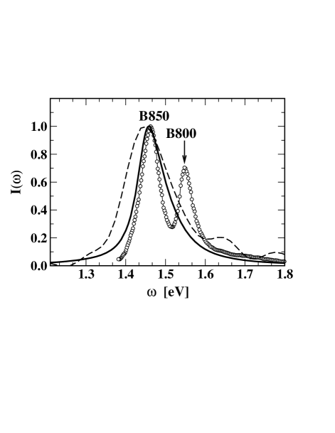
FIG. 13.: Normalized absorption spectra of the B850 BChls with excitonic coupling: $I_{B850}(\omega)$ – polaron model (solid curve), $I_{TSA}(\omega)$ – time series analysis (dashed curve) and $I_{exp}(\omega)$ – experiment (circles).

Within the framework of the polaron model, the absorption spectrum $I_{B850}(\omega)$ of the excitonically coupled B850 BChls can be calculated numerically by using Eqs. (166,V E,159,153,134). The needed input quantities are: $T=300$ K, ${\cal C}(t)$, and $\epsilon_{k}=\epsilon_{\pm 1}=1.52$ eV; these are derived from our simulations and there are no free parameters in the above mentioned equations. The computed $I_{B850}(\omega)$ is shown in Fig. 13, along with the corresponding spectrum $I_{TSA}(\omega)$ obtained through time series analysis, [c.f. Eqs. (64,65)], and the corresponding experimental result $I_{exp}(\omega)$ [42]. The peak of $I_{B850}$ is located at 1.46 eV ($\approx 849$ nm), and coincides with the position of the other two spectra. $I_{B850}(\omega)$ (FWHM=88 meV) is somewhat broader than $I_{exp}(\omega)$ (FWHM=58 meV), but is narrower than $I_{TSA}(\omega)$ (FWHM=138 meV). The effect of exchange narrowing due to the excitonic coupling between B850 BChls is manifest: FWHM is reduced from 154 meV (Fig. 13) to 88 meV (Fig. 12a), which represents a reduction in the width of the line shape function by a factor of 1.75. This exchange narrowing is accounted for by the factor $F_{k}(t)$ in Eq. (141); since $|F_{k}(t)|\leq 1$, this factor reduces the value of the cumulant $\Phi_{k}(t)$, which leads to a narrowing of the line shape function [recall that $\Phi_{k}=0$ result in a Dirac-delta function type $I(\omega)$]. In contrast to the commonly used stochastic models [58] for describing the absorption spectrum of molecular aggregates, our polaron model does not postulate the form of the autocorrelation function ${\cal C}(t)$, but rather uses this function as an input, derived from computer simulations or from experiment. In this regard, our polaron model provides a more realistic approach for evaluating optical properties of molecular aggregates in general, and the B850 excitons in particular. Indeed, a generic autocorrelation function ${\cal C}(t)=\Delta^{2}\exp(-\lambda t)$, assumed by most stochastic models, would represent a gross oversimplification of the complicated structure of ${\cal C}(t)$ as inferred from our computer simulations (see Fig. 11a). It is clear that this autocorrelation function cannot be modeled by either a single or a sum of several exponentially decaying functions, in spite of the fact that by a proper choice of the values of the mean square fluctuations of the energy gap, $\Delta^{2}$, and of the inverse relaxation time, $\lambda$, the stochastic model can yield an almost perfect fit to the experimental spectrum. For example, by assuming that in our case the broadening of the line shape function is due to coupling to phonons with clearly separated high and low frequency components, it can be shown that the real part of the cumulant is approximately $\Phi^{\prime}(t)\approx\Delta_{\ell}^{2}t^{2}/2+\Gamma_{h}t$, where $\ell$ ($h$) refers to the low (high) frequency component and $\Gamma_{h}=\Delta_{h}^{2}/\lambda_{h}$. (The imaginary part of the cumulant $\Phi^{\prime\prime}(t)$ is assumed to affect only the shift of the absorption spectrum, but not its broadening.) The first (second) term in $\Phi^{\prime}(t)$ represents the short (long) time approximation of the cumulant brought about by the low (high) frequency phonons. The corresponding line shape function has a Voigt profile [58], i.e., is a convolution of a Gaussian and Lorentzian due to low and high frequency phonons, respectively. For $\Delta_{s}=25$ meV and $\Gamma_{\ell}=7$ meV, one can obtain an almost perfect fit to the experimental B850 absorption spectrum. However, in spite of this apparent agreement with experiment, neither these numerical values nor the clear separation in the phonon spectral density is justified in view of our computer simulation results, and as such this kind of analysis should be avoided. In fact, as it can be inferred from the plot of $J(\omega)$ shown in Fig. 11b, all phonon frequencies up to 0.24 eV contribute to the cumulant $\Phi(t)$ and, therefore, to the absorption spectrum $I(\omega)$. Thus, unlike stochastic models which employ fitting parameters to account for the broadening of the experimental absorption spectra, our polaron model incorporates dynamic disorder directly through the phonon spectral function $J(\omega)$ obtained from combined MD/quantum chemistry calculations, i.e., without any ad hoc assumptions and fitting parameters.

Further tests of our polaron model based on the calculation of other optical properties of the system, such as the circular dichroism (CD) spectrum, are in preparation.

VI Discussion

This paper presents a novel approach to the study of excitons in light-harvesting complexes that combines molecular dynamics and quantum chemistry calculations with time-dependent effective Hamiltonian as well as polaron model type of analyses.

The molecular dynamics approach allowed us to observe, at the atomic level, the dynamics of BChl motions and gain insight into the extent and timescales of geometrical deformations of pigment and protein residues at physiological temperatures. A comparison of the average distances and angles between the B850 BChls to those found in the crystal structure reveals an increased dimerization within the B850 ring, as compared to the crystal structure. We observed diffusion of a water molecule into the B800 BChl binding site for seven out of eight B800 BChls. The average location of this water molecule agrees well with the crystal structure location. Future quantum chemistry calculations will determine whether this molecule plays a functional role. In this respect it is interesting to note that the recently published structure of the cyanobacterial photosystem I at 2.5 Åresolution revealed also ligations of Chla Mg ions involving side groups other than His, and, in particular, water [59].

The time series analysis theory, based on the combined MD/QC calculations resulted in an absorption spectrum that is about a factor of two wider than the experimental spectrum. One of the reasons for this discrepancy might be improper treatment, and subsequently an overestimate, of the contribution of high-frequency modes within the framework of our combined MD/QC calculations. We also note that the time series analysis neglects some important quantum effects which may cause the discrepancy between the computed and the experimental results. These quantum effects are accounted for by the polaron model. The amplitude of fluctuations of the off-diagonal matrix elements, i.e., couplings between BChls, was found to be at least two orders of magnitude smaller than the corresponding fluctuation amplitude of the diagonal matrix elements. We believe that in spite of the possible overestimate of the fluctuation associated with the high frequency modes, we can safely conclude that the disorder in the B850 system is diagonal rather than off-diagonal in nature.

The time-dependent effective Hamiltonian description revealed an exciton spectrum red-shifted as compared to the spectrum of individual BChls. This red-shift is well known in J-aggregates, and is attributed to the transferring of the dipole strength into low-energy exciton states.

The observation that the fluctuations of the BChl site energies could be attributed largely to high frequency intramolecular vibrational modes, with energy $\omega_{0}\sim 1,600-1,700$ cm^-1, prompted us to model the effect of dynamic disorder on the B850 excitons by employing a polaron Hamiltonian, which describes both excitons and the coupled single phonon mode by quantum mechanics. The strength of the exciton-phonon coupling $g$ is related to the RMSD of the fluctuating site energies, and was found to be weak. By employing standard perturbation theory we investigated the effect of dynamic disorder (i.e., exciton-phonon coupling) on the energy dispersion and localization of the excitons. We found that in contrast to static disorder, which leads to a broadening of the exciton bandwidth, dynamic disorder due to high frequency vibrational modes leads to a reduction of the width of the exciton energy band. Also, our polaron calculations showed that dynamic disorder reduces only slightly the exciton delocalization length (from around 6 BChls to 5 BChls at room temperature), confirming previous results according to which the main mechanism responsible for exciton localization in LH-II rings is thermal averaging [14].

By employing the cumulant expansion method, we calculated, in the framework of the polaron model, the absorption spectrum of the B850 BChl, with and without exciton coupling, for a single phonon mode as well as for a distribution of phonons. The absorption spectrum of the excitonic system coupled to a single high frequency phonon $\omega_{0}$ (intramolecular vibronic mode) is given by a series of Dirac-delta functions (stick spectrum), with different weights. In order to obtain a realistic, broadened absorption spectrum, which can be compared with the one measured experimentally we had to included the effect of the entire phonon distribution through the phonon spectral density $J(\omega)$. We have shown that $J(\omega)$, which accounts for both coupling strengths and frequencies of the individual phonon components, can be determined from the autocorrelation function ${\cal C}(t)$ of the energy gap fluctuations of individual BChls, readily available from our combined MD/quantum chemistry simulation. We found that in our model only three inputs, namely autocorrelation function ${\cal C}(t)$, temperature $T$ and optically active exciton level $\epsilon_{k}$, are needed to calculate the absorption spectrum. Considering the fact that these inputs come directly from our MD/QC calculations, and that we have no free parameters, the agreement between the spectrum obtained from the polaron model calculations and the experimental spectrum is remarkable.

- [1] R. van Grondelle, J. Dekker, T. Gillbro, and V. Sundström, Biochim. Biophys. Acta 1187, 1 (1994).
- [2] X. Hu and K. Schulten, Physics Today 50, 28 (1997).
- [3] X. Hu, A. Damjanović, T. Ritz, and K. Schulten, Proc. Natl. Acad. Sci. USA 95, 5935 (1998).
- [4] V. Sundström, T. Pullerits, and R. van Grondelle, J. Phys. Chem. B 103, 2327 (1999).
- [5] G. McDermott et al., Nature 374, 517 (1995).
- [6] J. Koepke et al., Structure 4, 581 (1996).
- [7] X. Hu, T. Ritz, A. Damjanović, and K. Schulten, J. Phys. Chem. B 101, 3854 (1997).
- [8] W. F. Humphrey, A. Dalke, and K. Schulten, J. Mol. Graphics 14, 33 (1996).
- [9] A. Gall, G. J. S. Fowler, C. N. Hunter, and B. Robert, Biochemistry 36, 16282 (1997).
- [10] J. N. Sturgis and B. Robert, Photosynthesis Research 50, 5 (1996).
- [11] A. S. Davydov, Theory of Molecular Excitons (McGraw-Hill, New York, 1962).
- [12] S. Karrasch, P. Bullough, and R. Ghosh, EMBO J. 14, 631 (1995).
- [13] T. Meier, Y. Zhao, V. Chernyak, and S. Mukamel, J. Chem. Phys. 107, 3876 (1997).
- [14] J. Ray and N. Makri, J. Phys. Chem. A 103, 9417 (1999).
- [15] D. Leupold et al., Phys. Rev. Lett. 77, 4675 (1996).
- [16] M. H. C. Koolhaas, G. van der Zwan, R. N. Frese, and R. van Grondelle, J. Phys. Chem. B 101, 7262 (1997).
- [17] J. T. M. Kennis et al., J. Phys. Chem. B 101, 8369 (1997).
- [18] R. Monshouwer, M. Abrahamsson, F. van Mourik, and R. van Grondelle, J. Phys. Chem. B 101, 7241 (1997).
- [19] T. Pullerits, M. Chachisvillis, and V. Sundström, J. Phys. Chem. 100, 10787 (1996).
- [20] M. Yang, R. Agarwal, and G. R. Fleming, ”J. Photochem. Photobiol. A” in press (2001).
- [21] A. van Oijen et al., Science 285, 400 (1999).
- [22] R. Jimenez, F. van Mourik, J. Y. Yu, and G. R. Fleming, J. Phys. Chem. B 101, 7350 (1997).
- [23] V. May and O. Kühn, Charge and Energy Transfer Dynamics in Molecular Systems (WILEY-VCH, Berlin, 2000).
- [24] M. J. Frisch et al., Gaussian 98, Revision A7, Gaussian Inc., Pittsburgh, PA, 1998.
- [25] G. Baym, Lectures on Quantum Mechanics (W. A. Benjamin, Inc., Reading, Mass., 1973).
- [26] K. J. Visscher et al., Biochemistry 30, 5734 (1991).
- [27] C. H. Wang, Spectroscopy of Condensed Media (Academic Press, Inc., Orlando, Florida, 1985).
- [28] A. T. Brünger, X-PLOR, Version 3.1: A System for X-ray Crystallography and NMR, The Howard Hughes Medical Institute and Department of Molecular Biophysics and Biochemistry, Yale University, 1992.
- [29] QUANTA 97, Molecular Simulations Inc., Burlington, Massachusetts, 1997.
- [30] H. Heller, M. Schaefer, and K. Schulten, J. Phys. Chem. 97, 8343 (1993).
- [31] A. D. MacKerell Jr. et al., FASEB J. 6:A143 (1992).
- [32] A. D. MacKerell Jr. et al., J. Phys. Chem. B 102, 3586 (1998).
- [33] W. L. Jorgensen et al., J. Chem. Phys. 79, 926 (1983).
- [34] M. M. Teeter, Ann. Rev. Biophys. Biophys. Chem. 20, 577 (1991).
- [35] V. Daggett and M. Levitt, Ann. Rev. Biophys. Biomol. Struct. 22, 353 (1993).
- [36] P. J. Steinbach and B. R. Brooks, Proc. Natl. Acad. Sci. USA 90, 9135 (1993).
- [37] M. N. Ringnalda et al., PS-GVB v2.3, Schrödinger Inc., Portland, OR, 1996.
- [38] N. Foloppe, J. Breton, and J. C. Smith, in The Photosynthetic Bacterial Reaction Center II: Structure, Spectroscopy and Dynamics, edited by J. Breton and A. Vermeglio (Plenum Press, New York and London, 1992), pp. 43–48.
- [39] N. Foloppe, M. Ferrand, J. Breton, and J. C. Smith, PROTEINS: Struc., Func., and Genetics 22, 226 (1995).
- [40] L. Kalé et al., J. Comp. Phys. 151, 283 (1999).
- [41] I. P. Mercer, I. R. Gould, and D. R. Klug, J. Phys. Chem. B 103, 7720 (1999).
- [42] J.-P. Zhang et al., J. Phys. Chem. B 104, 3683 (2000).
- [43] P. O. J. Scherer, in J-Aggregates, edited by T. Kobayashi (World Scientific, Singapore, 1996), pp. 95–110.
- [44] M. Wubs and J. Knoester, Chem. Phys. Lett. 284, 63 (1998).
- [45] M. G. Cory, M. C. Zerner, X. Hu, and K. Schulten, J. Phys. Chem. B 102, 7640 (1998).
- [46] S. Tretiak, C. Middleton, V. Chernyak, and S. Mukamel, J. Phys. Chem. B 104, 4519 (2000).
- [47] M. H. C. Koolhaas et al., Biochemistry 37, 4693 (1998).
- [48] B. P. Krueger, G. D. Scholes, and G. R. Fleming, J. Phys. Chem. B 102, 5378 (1998).
- [49] G. Scholes, I. Gould, R. Cogdell, and G. Fleming, J. Phys. Chem. B 103, 2543 (1999).
- [50] R. G. Alden et al., J. Phys. Chem. B 101, 4467 (1997).
- [51] J. Linnanto, J. E. I. Korppi-Tommola, and V. M. Helenius, J. Phys. Chem. B 103, 8739 (1999).
- [52] T. Holstein, Ann. Phys.(N.Y.) 8, 343 (1959).
- [53] G. D. Mahan, Many-Particle Physics, 2nd ed. (Plenum Press, New York, 1990).
- [54] S. Nakajima, Y. Toyozawa, and R. Abe, The Physics of Elementary Excitations (Springer-Verlag, Berlin, 1980).
- [55] E. N. Economou, Green’s Functions in Quantum Physics (Springer, New York, 1983).
- [56] D. Xu and K. Schulten, Chem. Phys. 182, 91 (1994).
- [57] K. Ohta, D. S. Larsen, M. Yang, and G. R. Fleming, J. Chem. Phys. 114, 8020 (2001).
- [58] S. Mukamel, Principles of nonlinear optical spectroscopy (Oxford University Press, New York, 1995).
- [59] P. Jordan et al., Nature 411, 909 (2001).