Quantum Clustering

Abstract

We propose a novel clustering method that is based on physical intuition derived from quantum mechanics. Starting with given data points, we construct a scale-space probability function. Viewing the latter as the lowest eigenstate of a Schrödinger equation, we use simple analytic operations to derive a potential function whose minima determine cluster centers. The method has one parameter, determining the scale over which cluster structures are searched. We demonstrate it on data analyzed in two dimensions (chosen from the eigenvectors of the correlation matrix). The method is applicable in higher dimensions by limiting the evaluation of the Schrödinger potential to the locations of data points. In this case the method may be formulated in terms of distances between data points.

1 Introduction

Clustering of data is a well-known problem of pattern recognition, covered in textbooks such as [1, 2, 3]. The problem we are looking at is defining clusters of data solely by the proximity of data points to one another. This problem is one of unsupervised learning, and is in general ill defined. Solutions to such problems can be based on intuition derived from Physics. A good example of the latter is the algorithm by [4] that is based on associating points with Potts-spins and formulating an appropriate model of statistical mechanics. We propose an alternative that is also based on physical intuition, this one being derived from quantum mechanics.

As an introduction to our approach we start with the scale-space algorithm by [5] who uses a Parzen-window estimator[3] of the probability distribution leading to the data at hand. The estimator is constructed by associating a Gaussian with each of the $N$ data points in a Euclidean space of dimension $d$ and summing over all of them. This can be represented, up to an overall normalization by

$$\psi({\bf x})=\sum_{i}e^{-{({\bf x-x}_{i})^{2}\over 2\sigma^{2}}}$$ (1)

where ${\bf x}_{i}$ are the data points. Roberts [5] views the maxima of this function as determining the locations of cluster centers.

An alternative, and somewhat related method, is Support Vector Clustering (SVC) [6] that is based on a Hilbert-space analysis. In SVC one defines a transformation from data space to vectors in an abstract Hilbert space. SVC proceeds to search for the minimal sphere surrounding these states in Hilbert space.We will also associate data-points with states in Hilbert space. Such states may be represented by Gaussian wave-functions, in which case $\psi({\bf x})$ is the sum of all these states. This is the starting point of our method. We will search for the Schrödinger potential for which $\psi({\bf x})$ is a ground-state. The minima of the potential define our cluster centers.

2 The Schrödinger Potential

We wish to view $\psi$ as an eigenstate of the Schrödinger equation

$$H\psi\equiv(-{\sigma^{2}\over 2}\nabla^{2}+V({\bf x}))\psi=E\psi.$$ (2)

Here we rescaled $H$ and $V$ of the conventional quantum mechanical equation to leave only one free parameter, $\sigma$. For comparison, the case of a single point at ${\bf x}_{1}$ corresponds to Eq. 2 with $V={1\over 2\sigma^{2}}({\bf x-x}_{1})^{2}$ and $E=d/2$, thus coinciding with the ground state of the harmonic oscillator in quantum mechanics.

Given $\psi$ for any set of data points we can solve Eq. 2 for $V$:

$$V({\bf x})=E+{{\sigma^{2}\over 2}\nabla^{2}\psi\over\psi}=E-{d\over 2}+{1\over 2\sigma^{2}\psi}\sum_{i}({\bf x}-{\bf x}_{i})^{2}e^{-{({\bf x-x}_{i})^{2}\over 2\sigma^{2}}}$$ (3)

Let us furthermore require that min$V$=0. This sets the value of

$$E=-{\rm min}{{\sigma^{2}\over 2}\nabla^{2}\psi\over\psi}$$ (4)

and determines $V({\bf x})$ uniquely. $E$ has to be positive since $V$ is a non-negative function. Moreover, since the last term in Eq. 3 is positive definite, it follows that

$$0<E\leq{d\over 2}\,.$$ (5)

We note that $\psi$ is positive-definite. Hence, being an eigenfunction of the operator $H$ in Eq. (2), its eigenvalue $E$ is the lowest eigenvalue of $H$, i.e. it describes the ground-state. All higher eigenfunctions have nodes whose number increases as their energy eigenvalues increase.

Given a set of points defined within some region of space, we expect $V({\bf x})$ to grow quadratically outside this region, and to exhibit one or several local minima within the region. Just as in the harmonic potential of the single point problem, we expect the ground-state wave-function to concentrate around the minima of the potential $V({\bf x})$. Therefore we will identify these minima with cluster centers.

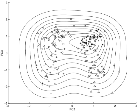
Figure 1: Ripley’s crab data [7] displayed on a plot of their 2nd and 3rd principal components with a superimposed topographic map of the Roberts’ probability distribution for $\sigma=1/\sqrt{2}$.

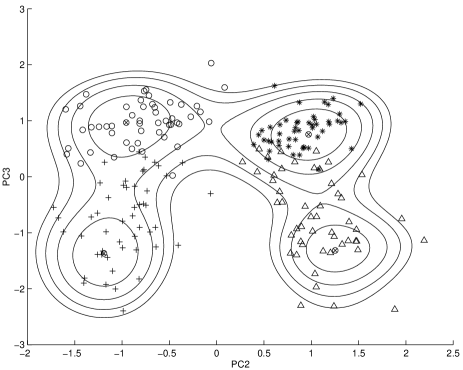
Figure 2: A topographic map of the potential for the crab data with $\sigma=1/\sqrt{2}$, displaying four minima (denoted by crossed circles) that are interpreted as cluster centers. The contours of the topographic map are set at values of $V({\bf x})/E=.2,.4,.6,.8,1.$

As an example we display results for the crab data set taken from Ripley’s book [7]. These data, given in a five-dimensional parameter space, show nice separation of the four classes contained in them when displayed in two dimensions spanned by the 2nd and 3rd principal components[8] (eigenvectors) of the correlation matrix of the data. The information supplied to the clustering algorithm contains only the coordinates of the data-points. We display the correct classification to allow for visual comparison of the clustering method with the data. Starting with $\sigma=1/\sqrt{2}$ we see in Fig. 1 that the Parzen probability distribution, or the wave-function $\psi$, has only a single maximum. Nonetheless, the potential, displayed in Fig. 2, shows already four minima at the relevant locations. The overlap of the topographic map of the potential with the true classification is quite amazing. The minima are the centers of attraction of the potential, and they are clearly evident although the wave-function does not display local maxima at these points. The fact that $V({\bf x})=E$ lies above the range where all valleys merge explains why $\psi({\bf x})$ is smoothly distributed over the whole domain.

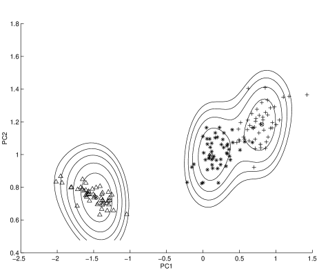
Figure 3: Quantum clustering of the iris data for $\sigma=1/4$ in a space spanned by the first two principal components. Different symbols represent the three classes. Equipotential lines are drawn at $V({\bf x})/E=.2,.4,.6,.8,1.$

We ran our method also on the iris data set [9], which is a standard benchmark obtainable from the UCI repository [10]. The data set contains 150 instances each composed of four measurements of an iris flower. There are three types of flowers, represented by 50 instances each. Clustering of these data in the space of the first two principal components is depicted in Figure 3. The results shown here are for $\sigma=1/4$ which allowed for clustering that amounts to misclassification of three instances only, quite a remarkable achievement (see, e.g. [6]).

3 Application of Quantum Clustering

The examples displayed in the previous section show that, if the spatial representation of the data allows for meaningful clustering using geometric information, quantum clustering (QC) will do the job. There remain, however, several technical questions to be answered: What is the preferred choice of $\sigma$? How can QC be applied in high dimensions? How does one choose the appropriate space, or metric, in which to perform the analysis? We will confront these issues in the following.

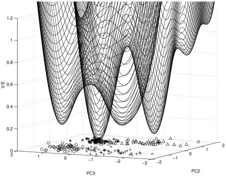
Figure 4: The potential for the crab data with $\sigma=1/2$ is displayed on a three-dimensional plot of $V({\bf x})$ in units of $E$, the ground-state energy. Two additional, but insignificant, minima appear. The four deep minima are roughly at the same locations as in Fig. 2.

In the crabs-data of we find that as $\sigma$ is decreased to ${1\over 2}$, the previous minima of $V({\bf x})$ get deeper and two new minima are formed. However the latter are insignificant, in the sense that they lie at high values (of order $E$), as shown in Fig. 4. Thus, if we classify data-points to clusters according to their topographic location on the surface of $V({\bf x})$, roughly the same clustering assignment is expected for $\sigma={1\over 2}$ as for ${1\over\sqrt{2}}$. One important advantage of quantum clustering is that $E$ sets the scale on which minima are observed. Thus, we learn from Fig. 2 that the cores of all four clusters can be found at $V$ values below $.4E$. The same holds for the significant minima of Fig. 4.

By the way, the wave function acquires only one additional maximum at $\sigma={1\over 2}$. As $\sigma$ is being further decreased, more and more maxima are expected in $\psi$ and an ever increasing number of minima (limited by $N$) in $V$.

The one parameter of our problem, $\sigma$, signifies the distance that we probe. Accordingly we expect to find clusters relevant to proximity information of the same order of magnitude. One may therefore vary $\sigma$ continuously and look for stability of cluster solutions, or limit oneself to relatively low values of $\sigma$ and decide to stop the search once a few clusters are being uncovered.

4 Principal Component Metrics

In all our examples data were given in some high-dimensional space and we have analyzed them after defining a projection and a metric, using the PCA approach. The latter defines a metric that is intrinsic to the data, determined by their second order statistics. But even then, several possibilities exist, leading to non-equivalent results.

Principal component decomposition can be applied both to the correlation matrix $C_{\alpha\beta}=<x_{\alpha}x_{\beta}>$ and to the covariance matrix

$${\cal C}_{\alpha\beta}=<(x_{\alpha}-<x>_{\alpha})(x_{\beta}-<x>_{\beta})>=C_{\alpha\beta}-<x>_{\alpha}<x>_{\beta}\,.$$ (6)

In both cases averaging is performed over all data points, and the indices indicate spatial coordinates from 1 to $d$. The principal components are the eigenvectors of these matrices. Thus we have two natural bases in which to represent the data. Moreover one often renormalizes the eigenvector projections, dividing them by the square-roots of their eigenvalues. This procedure is known as “whitening”, leading to a renormalized correlation or covariance matrix of unity. This is a scale-free representation, that would naturally lead one to start with $\sigma=1$ in the search for (higher-order) structure of the data.

The PCA approach that we have used on our examples was based on whitened correlation matrix projections. This turns out to produce good separation of crab-data in PC2-PC3 and of iris-data in PC1-PC2. Had we used the covariance matrix ${\bf\cal C}$ instead, we would get similar, but slightly worse, separation of crab-data, and a much worse representation of the iris-data. Our examples are meant to convince the reader that once a good metric is found, QC conveys the correct information. Hence we allowed ourselves to search first for the best geometric representation, and then apply QC.

5 QC in Higher Dimensions

In the iris problem we obtained excellent clustering results using the first two principal components, whereas in the crabs problem, clustering that depicts correctly the classification necessitates components 2 and 3. However, once this is realized, it does not harm to add the 1st component. This requires working in a 3-dimensional space, spanned by the three leading PCs. Increasing dimensionality means higher computational complexity, often limiting the applicability of a numerical method. Nonetheless, here we can overcome this “curse of dimensionality” by limiting ourselves to evaluating $V$ at locations of data-points only. Since we are interested in where the minima lie, and since invariably they lie near data points, no harm is done by this limitation. The results are depicted in Fig. 5. Shown here are $V/E$ values as function of the serial number of the data, using the same symbols as in Fig. 2 to allow for visual comparison. Using all data of $V<0.3E$ one obtains cluster cores that are well separated in space, corresponding to the four classes that exist in the data. Only 9 of the 129 points that obey $V<0.3E$ are misclassified by this procedure. Adding higher PCs, first component 4 and then component 5, leads to deterioration in clustering quality. In particular, lower cutoffs in $V/E$, including lower fractions of data, are required to define cluster cores that are well separated in their relevant spaces.

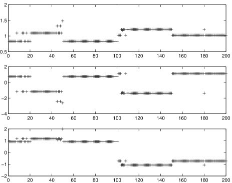
Figure 6: The results of gradient-descent dynamics applied to the 3D problem presented in Fig. 5. Shown here are values of the three coordinates (the three PCs) in three windows, as function of the serial number of the data. One clearly observes four clusters. But for the first class of data (the first 50 points), all clusters agree quite well with the classes. The first class, although belonging mostly to a separate cluster, has a large overlap with the cluster of the second class. Three points (numbers 45, 48 and 50) do not belong to any of the four clusters.

One may locate the cluster centers, and deduce the clustering allocation of the data, by following dynamics of gradient descent into the potential minima. Defining ${\bf y}_{i}(0)={\bf x}_{i}$ one follows steps of ${\bf y}_{i}(t+\Delta t)={\bf y}_{i}(t)-\eta(t)\nabla V({\bf y}_{i}(t))$, letting the points ${\bf y}_{i}$ reach an asymptotic fixed value coinciding with a cluster center. More sophisticated minimum search algorithms (see, e.g. chapter 10 in [11]) can be applied to reach the fixed points faster. The results of a gradient-descent procedure, applied to the 3D analysis of the crabs data shown in Fig. 5, is displayed in Fig. 6. One clearly observes the four clusters, and can compare clustering allocation with the original data classes.

6 Distance-based QC Formulation

Gradient descent calls for the calculation of $V$ both on the original data-points, as well as on the trajectories they follow. An alternative approach can be to restrict oneself to the original values of $V$, as in the example displayed in Figure 5, and follow a hybrid algorithm to be described below. Before turning to such an algorithm let us note that, in this case, we evaluate $V$ on a discrete set of points $V({\bf x}_{i})=V_{i}$. We can then express $V$ in terms of the distance matrix $D_{ij}=|{\bf x}_{i}-{\bf x}_{j}|$ as

$$V_{i}=E-{d\over 2}+{1\over 2\sigma^{2}}{\sum_{j}D_{ij}^{2}e^{-{D_{ij}^{2}\over 2\sigma^{2}}}\over\sum_{j}e^{-{{D_{ij}^{2}}\over 2\sigma^{2}}}}$$ (7)

with $E$ chosen appropriately so that min$V_{i}$=0. This kind of formulation is of particular importance if the original information is given in terms of distances between data points rather than their locations in space. In this case we have to proceed with distance information only.

Applying QC we can reach results of the type of Fig. 5 without invoking any explicit spatial distribution of the points in question. One may then analyze the results by choosing a cutoff, e.g. $V<0.2E$, such that a fraction (e.g. $1/3$) of the data will be included. On this subset select groups of points whose distances from one another are smaller than, e.g., 2$\sigma$, thus defining cores of clusters. Then continue with higher values of $V$, e.g. $0.2E<V<0.4E$, allocating points to previous clusters or forming new cores. Since the choice of distance cutoff in cluster allocation is quite arbitrary, this method cannot be guaranteed to work as well as the gradient-descent approach.

7 Generalization

Our method can be easily generalized to allow for different weighting of different points, as in

$$\psi({\bf x})=\sum_{i}c_{i}e^{-{({\bf x-x}_{i})^{2}\over 2\sigma^{2}}}$$ (8)

with $c_{i}\geq 0$. This is important if we have some prior information or some other means for emphasizing or deemphasizing the influence of data points. An example of the latter is using QC in conjunction with SVC [6]. SVC has the possibility of labelling points as outliers. This is done by applying quadratic maximization to the Lagrangian

$$W=1-\sum_{i,j}\beta_{i}\beta_{j}e^{-{({\bf x}_{i}-{\bf x}_{j})^{2}\over 2\sigma^{2}}}$$ (9)

over the space of all $0\leq\beta_{i}\leq{1\over pN}$ subject to the constraint $\sum_{i}\beta_{i}=1$. The points for which the upper bound of $\beta_{i}$ is reached are labelled as outliers. Their number is regulated by $p$, being limited by $pN$. Using for the QC analysis a choice of $c_{i}={1\over pN}-\beta_{i}$ will eliminate the outliers of SVC and emphasize the role of the points expected to lie within the clusters.

8 Discussion

QC constructs a potential function $V({\bf x})$ on the basis of data-points, using one parameter, $\sigma$, that controls the width of the structures that we search for. The advantage of the potential $V$ over the scale-space probability distribution is that the minima of the former are better defined (deep and robust) than the maxima of the latter. However, both of these methods put the emphasis on cluster centers, rather than, e.g., cluster boundaries. Since the equipotentials of $V$ may take arbitrary shapes, the clusters are not spherical, as in the k-means approach. Nonethelss, spherical clusters appear more naturally than, e.g., ring-shaped or toroidal clusters, even if the data would accomodate them. If some global symmetry is to be expected, e.g. global spherical symmetry, it can be incorporated in the original Schrödinger equation defining the potential function.

QC can be applied in high dimensions by limiting the evaluation of the potential, given as an explicit analytic expression of Gaussian terms, to locations of data points only. Thus the complexity of evaluating $V_{i}$ is of order $N^{2}$ independently of dimensionality. Our algorithm has one free parameter, the scale $\sigma$. In all examples we confined ourselves to scales that are of order 1, because we have worked within whitened PCA spaces. If our method is applied to a different data-space, the range of scales to be searched for could be determined by some other prior information.

Since the strength of our algorithm lies in the easy selection of cluster cores, it can be used as a first stage of a hybrid approach employing other techniques after the identification of cluster centers. The fact that we do not have to take care of feeble minima, but consider only robust deep minima, turns the identification of a core into an easy problem. Thus, an approach that drives its rationale from physical intuition in quantum mechanics, can lead to interesting results in the field of pattern classification.

We thank B. Reznik for a helpful discussion.

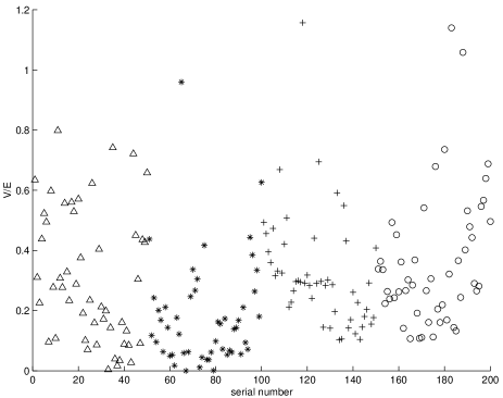
Figure 5: Values of $V({\bf x})/E$ are depicted in the crabs problem with three leading PCs for $\sigma=1/2$. They are presented as function of the serial number of data, using the same symbols of data employed before. One observes low lying data of all four classes.

References

- [1] A.K. Jain and R.C. Dubes. Algorithms for clustering data. Prentice Hall, Englewood Cliffs, NJ, 1988.
- [2] K. Fukunaga. Introduction to Statistical Pattern Recognition. Academic Press, San Diego, CA, 1990.
- [3] R.O. Duda, P.E. Hart and D.G. Stork. Pattern Classification. Wiley-Interscience, 2nd ed., 2001.
- [4] M. Blat, S. Wiseman and E. Domany. Phys. Rev. Letters 76 3251 (1996).
- [5] S.J. Roberts. Pattern Recognition, 30 261 (1997).
- [6] A. Ben-Hur, D. Horn, H.T. Siegelmann, and V. Vapnik. Neural Information Processing Systems 2000.
- [7] B. D. Ripley Pattern Recognition and Neural Networks. Cambridge University Press, Cambridge UK, 1996.
- [8] I. T. Jolliffe Principal Component Analysis. Springer Verlag, New York, 1986.
- [9] R.A. Fisher. Annual Eugenics, 7,II 179 (1936).
- [10] C.L. Blake and C.J. Merz. UCI Repository of machine learning databases, 1998.
- [11] W. H. Press, S. A. Teuklosky, W. T. Vetterling and B. P. Flannery. Numerical Recipes - The Art of Scientific Computing 2nd ed. Cambridge Univ. Press, 1992.