Mean flow in hexagonal convection: stability and nonlinear dynamics

Abstract

Weakly nonlinear hexagon convection patterns coupled to mean flow are investigated within the framework of coupled Ginzburg-Landau equations. The equations are in particular relevant for non-Boussinesq Rayleigh-Bénard convection at low Prandtl numbers. The mean flow is found to (1) affect only one of the two long-wave phase modes of the hexagons and (2) suppress the mixing between the two phase modes. As a consequence, for small Prandtl numbers the transverse and the longitudinal phase instability occur in sufficiently distinct parameter regimes that they can be studied separately. Through the formation of penta-hepta defects, they lead to different types of transient disordered states. The results for the dynamics of the penta-hepta defects shed light on the persistence of grain boundaries in such disordered states.

1 Introduction

Roll patterns in Rayleigh-Bénard convection of a fluid layer heated from below have been explored extensively over the years as a paradigmatic system to study the succession of transitions from ordered to disordered and eventually turbulent states (for a recent review see [1]). Substantial theoretical effort has been devoted to identifying all the linear instabilities that straight roll patterns can undergo (e.g. [2]). Depending on the wavenumber of the roll pattern, the temperature difference across the layer (Rayleigh number), and the fluid properties (Prandtl number) a host of instabilities has been identified. The main instabilities being the Eckhaus, zig-zag, cross-roll, oscillatory, and skew-varicose instabilities. They limit the band of stable wavenumbers of straight rolls (Busse balloon). It turns out that the oscillatory and the skew-varicose instabilities depend sensitively on the Prandtl number and are relevant only if the Prandtl number is sufficiently small [2].

For small convection amplitudes a weakly nonlinear description in terms of a Newell-Whitehead-Segel equation [3, 4] would be expected to be sufficient at least for almost straight roll patterns. However, it is found that this is true only in the limit of large Prandtl numbers. It has been shown that slightly curved roll patterns drive a mean flow. Because of the incompressibility of the fluid it induces a non-local coupling of the rolls, which is not contained in the Newell-Whitehead-Segel equation [5]. The strength of the mean flow increases with decreasing Prandtl number. For small Prandtl numbers the Newell-Whitehead-Segel equation has therefore been extended to include an equation for the vertical vorticity characterizing the mean flow [5].

Experimentally, the mean flow has been observed in experiments in a relatively small circular container [6]. Since the usual boundary conditions require the convection rolls to be essentially perpendicular to the side-walls the rolls become strongly curved in this geometry. The resulting mean flow has been identified as the driving force for the observed persistent creation and annihilation of dislocations [7, 8, 9].

Arguably the most interesting state that is due to the mean flow associated with small Prandtl numbers is the spiral-defect chaos observed in large-aspect ratio experiments on thin gas layers [10]. It is characterized by the appearance of various types of defects in the pattern with small rotating spirals being the ones that are visually most striking. Spiral-defect chaos does not arise from a linear instability of the straight roll pattern and, in fact, bistability of straight roll patterns and spiral-defect chaos has been observed experimentally [11]. The onset of spiral-defect chaos depends strongly on the Prandtl number, indicating that mean flows play an essential role in maintaining this state [12, 13, 14, 15].

Motivated by the strong impact of mean flows on roll convection patterns we consider in this paper the effect of such flows on the stability and dynamics of hexagonal patterns. Hexagonal patterns are commonly found in spatially extended non-equilibrium systems such as non-Boussinesq Rayleigh-Bénard convection (e.g. [16]), Marangoni convection (e.g. [17]), Turing structures in chemical systems [18], crystal growth (e.g. [19]), and surface waves on vertically vibrated liquid or granular layers (Faraday experiment) [20, 21]. Not in all of these systems mean flows of the type discussed above arise. Clearly, they are relevant for the small Prandtl numbers in gas convection in very thin layers [10]. Interestingly, the skewed-varicose instability and a (transient) state similar to spiral-defect chaos have been observed also in vertically vibrated granular layers [22, 23]. Since in convection at low Prandtl numbers they are a signature of the importance of mean flow, mean flow may also be relevant in vertically vibrated fluids. We focus in this paper on patterns arising from a steady bifurcation, as is the case in convection. Immediately above onset, parametrically excited standing waves like those arising in the Faraday experiment behave in many respects like patterns that are due to a steady bifurcation (e.g. [24]). Our results may therefore also be relevant for hexagon patterns in suitable Faraday experiments.

In the absence of mean flows the stability of hexagonal patterns has been studied in detail in the weakly nonlinear regime. Starting from three coupled Ginzburg-Landau-type equations for the amplitudes of the rolls that make up the hexagonal pattern two coupled phase equations have been derived that describe the dynamics of long-wave deformations of the hexagon patterns [25, 26, 27, 28]. In these theoretical analyses two types of long-wave instabilities have been identified, a longitudinal and a transverse mode, with the longitudinal mode being relevant only for Rayleigh numbers very close to the saddle-node bifurcation at which the hexagons first appear. In a more detailed analysis also perturbations with arbitrary wavenumber and simulations of the nonlinear evolution ensuing from the instabilities have been included [29]. The instabilities typically lead to the formation of penta-hepta defects [30, 31]. Their dynamics and interaction has also been studied in the absence of mean flows [32, 33]. In the strongly nonlinear regime long-wave perturbations are still captured by phase equations [28]. Specifically for convection at large Prandtl numbers driven by a combination of buoyancy and surface tension the stability of hexagons and their dynamics has been investigated in [34]. Experimentally, the stability of hexagonal convection patterns has not been studied in detail. A contributing factor has been that controlled changes in the wavenumber of the pattern are considerably more difficult to effect than in systems like Taylor-vortex flow, where detailed agreement between experiment and theory has been achieved (e.g. [35, 36]). Recently, however, it has been possible to use localized heating as a printing technique for convection patterns [37, 38]. This will make detailed analyses of the wavenumber-dependent instabilities of hexagon patterns experimentally accessible.

         

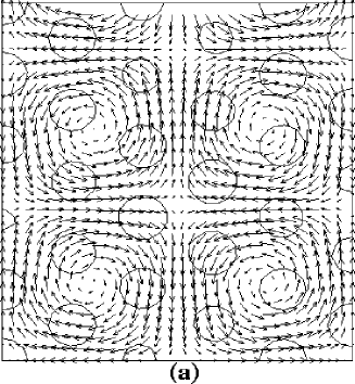
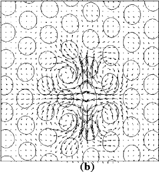
Figure 1: Illustration of the mean flow due to modulation of the hexagon envelope (panel(a)) or due to a penta-hepta defect (panel(b)). For visual clarity the wavelength of the hexagon pattern has been chosen larger (relative to the modulation wavelength) than is appropriate for the weakly nonlinear theory presented in this paper.

The goal of this study is to investigate the linear stability of hexagons coupled to a two-dimensional mean flow driven by modulations of the pattern and the nonlinear evolution arising from the instabilities. An example of the flow generated by two typical patterns is shown in fig.1a,b. In fig.1a a periodic hexagon pattern is sinusoidally modulated on a length scale five times the hexagon size and fig.1b shows the mean flow generated by a penta-hepta defect. The mean flow is found to couple only to one of the two long-wave modes. As a consequence, for sufficiently small Prandtl numbers each of the two long-wave instabilities dominates in a separate, experimentally accessible parameter regime. Both instabilities induce the formation of defects. We study their motion and briefly touch upon its impact on disordered patterns and grain boundaries.

The paper is organized as follows: first we formulate the problem extending previous work on the mean flow generated by roll convection [39, 40]. We then study the stability of the hexagonal pattern with respect to long-wave perturbations (sec.3) and with respect to general side-band perturbations (sec.4). In section 5 the nonlinear evolution of the instabilities including the formation, dynamics, and annihilation of defects is investigated. There, we also study the transition from hexagonal to roll patterns triggered by the side-band instabilities.

2 Amplitude equations

The interaction between weakly nonlinear convection rolls and the mean flow generated by them has been investigated for Rayleigh-Bénard convection with both no-slip and stress-free boundary conditions at the top and bottom plate [39, 40]. The relevant amplitude equations were derived and used to determine the stability of rolls with respect to side-band instabilities. Expanding the fluid velocity in terms of the complex amplitude $A$ of the convection rolls and the real streamfunction $Q$ for the two-dimensional mean flow as ($\epsilon\ll 1$),

$${\bf v}(\tilde{x},\tilde{y},\tilde{z},\tilde{t})=\epsilon A(x,y,t)e^{iq_{c}\tilde{x}}{\bf v}_{q}(\tilde{z})+\epsilon^{2}\left\{\vec{\nabla}\times(-Q\hat{z})f(\tilde{z})\right\}+h.o.t.,$$ (1)

the extended Ginzburg-Landau equation for $A$ and $Q$ is given by

$$\partial_{t}A = (\mu+(\partial_{x}-i\lambda\partial^{2}_{y})^{2}-|A|^{2})A-is_{1}A\partial_{y}Q+h.o.t.$$ (2)

$$M(Q) = 2q_{1}(\partial_{x}-i\lambda\partial^{2}_{y})\partial_{y}|A|^{2}+h.o.t.$$ (3)

where $\lambda\equiv\epsilon/2q_{c}$ with $\epsilon$ the supercriticality parameter and $q_{c}$ the critical wavenumber. Here $M(Q)=\nabla^{2}Q$ for no-slip boundary conditions [39] and $M(Q)=(q_{2}\nabla^{2}\partial_{t}-\nabla^{4})Q$ for the stress-free case [40]. It is worth noting that in the no-slip case the mean flow is not an additional dynamical variable and could in principle be adiabatically eliminated which would lead to a non-local equation for $A$. The slow time $t$ is given by $t=\epsilon^{2}\tilde{t}$. The non-isotropic Newell-Whitehead-Segel operator $(\partial_{x}-i\lambda\partial^{2}_{y})^{2}$ reflects the anisotropic scaling of the slow spatial scales $x=\epsilon\tilde{x}$ and $y=\epsilon^{1/2}\tilde{y}$. To leading order, the mean flow is driven by variations in the magnitude of the convective amplitude and couples back through the advective term $is_{1}A\partial_{y}Q=is_{1}AV_{x}$, where $V_{x}$ is the $x$-component of the mean flow. At higher orders a term of the form $V\cdot\nabla A$ would arise as well.

For the description of hexagonal convection patterns coupled to the mean flow the treatment has to be extended to include rolls in other directions than the $x$-axis. Using a coordinate transformation, it is straightforward to generalize the coupling term $A\partial_{y}Q$ for rolls in the $x$-direction $\hat{n}_{1}\equiv(1,0)$ to rolls in the other two hexagonal directions $\hat{n}_{2}\equiv(-1/2,\sqrt{3}/2)$ and $\hat{n}_{3}\equiv(-1/2,-\sqrt{3}/2)$. The amplitudes $A_{i}$, $i=1,2,3$, correspond then to rolls with wave vector $q_{c}\hat{n}_{i}$. For the generalization of the advection term $iA\partial_{y}Q$ in (2) it is convenient to introduce the unit vector $\hat{\tau}_{i}$ perpendicular to $\hat{n}_{i}$. To complete the extension of eqs.(2,3) from roll to hexagonal patterns we also add non-Boussinesq quadratic terms. For no-slip boundary conditions, the minimal set of equations describing hexagons coupled to a mean flow then reads

$$\partial_{t}A_{j} = \left(\mu+(\hat{n}_{j}\cdot\nabla)^{2}-|A_{i}|^{2}-\nu(|A_{j-1}|^{2}+|A_{j+1}|^{2})\right)A_{j}+$$ (4)

$$A_{j-1}^{*}A_{j+1}^{*}-i\beta A_{j}(\hat{\tau}_{j}\cdot\nabla)Q,$$

$$\nabla^{2}Q = -\left\{-2\partial_{xy}|A_{1}|^{2}+\right.$$ (5)

$$\left.\left[-\frac{\sqrt{3}}{2}(-\partial_{y}^{2}+\partial_{x}^{2})+\partial_{xy}\right]|A_{2}|^{2}+\left[\frac{\sqrt{3}}{2}(-\partial_{y}^{2}+\partial_{x}^{2})+\partial_{xy}\right]|A_{3}|^{2}\right\},$$

with cyclic permutation on $j$. It is not clear how the different scaling of the longitudinal spatial variable in the direction of $\hat{n}_{i}$ and of the transverse variable in the direction of $\hat{\tau}_{i}$ can be implemented in the hexagonal case where these directions are different for each of the three hexagon modes. We therefore use an isotropic scaling, $x=\epsilon\tilde{x}$ and $y=\epsilon\tilde{y}$, which renders the derivatives $i\lambda(\hat{\tau}_{j}\cdot\nabla)^{2}$ higher order in $\epsilon$. This can lead to degeneracies in certain growth rates like that of the zig-zag instability (e.g. [41, 42]). Then higher-order terms have to be re-introduced. For the hexagonal patterns this is, however, not the case. Note that while there is no direct damping of transverse variations, each of the $A_{j}$ is still allowed to vary in its respective transverse direction. This variation induces a variation in the longitudinal direction of the other two modes, in particular through the resonant interaction term $A_{j-1}^{*}A_{j+1}^{*}$, which then induces damping.

The cubic coefficient $\nu$ decreases monotonically with Prandtl number from $\nu\sim 2.0$ for $\mbox{\rm Pr}=0.5$ to $\nu\sim 1.5$ for $\mbox{\rm Pr}\sim 10$ [43, 16]. For the numerical results in this paper we fix $\nu=2$. Note that the mean flow amplitude $Q$ is of higher order than the hexagonal amplitudes, in fact, $Q\propto{\cal O}(A^{2})$. Nevertheless, the coupling term $iA(\hat{\tau}_{j}\cdot\nabla)Q$ is retained because $|\beta|$ can be much larger than one for low Prandtl number. For example, $\beta\sim-18$ for Prandtl number $\sim 0.1$ [39]. Furthermore, the mean flow introduces qualitatively new effects since it provides a non-local coupling between the convection amplitudes that is due to the incompressibility of the fluid.

In the absence of the mean flow, there exists a Lyapunov functional ${\cal F}$ for (4), which guarantees that only stationary patterns are possible as $t\rightarrow\infty$. Simple stationary solutions are:

$${\rm(i)\,\,rolls}\;\;\;A_{j}=(\mu-q^{2})^{1/2},\;\;A_{j\pm 1}=0,$$ (6)

$${\rm(ii)\,\,hexagons}\;\;\;A_{1}=A_{2}=A_{3}=\frac{1\pm\sqrt{1+4(\mu-q^{2})(1+2\nu)}}{2(1+2\nu)},$$ (7)

$${\rm(iii)\,\,mixed\,\,modes}\;\;\;A_{j}=\frac{1}{\nu-1},\;\;A_{j\pm 1}=\sqrt{\frac{\mu-q^{2}-A_{1}^{2}}{1+\nu}}.$$ (8)

As usual, the hexagon solution given by equation (7) with a minus sign in front of the square root is not stable. Thus, in the following we focus on the hexagon solution with the plus sign.

Since the mean flow couples to hexagons only through a modulation in the amplitudes, the stationary states (6-8) with constant amplitudes are also solutions to equations (4,5). However, their stability is modified by the coupling to the mean flow. In the case of rolls it can lead to an oscillatory instability (oscillatory skew-varicose instability), implying that there is no Lyapunov functional when taking the mean flow into account.

3 Linear Stability Analysis: Long-wave Approximation

We conduct a linear stability analysis of the hexagonal pattern (7) in the long-wave limit following the procedures in [26]. The amplitudes are perturbed around a hexagon pattern,

$$A_{j}=R_{0}e^{iq\hat{n}_{j}\cdot(x,y)}(1+r_{j}+i\phi_{j}),\;\;j=1,\;2,\;3,$$ (9)

where $R_{0}\equiv\left(1+\sqrt{1+4(\mu-q^{2})(1+2\nu)}\right)/2(1+2\nu)$ is the amplitude of the stationary solution with reduced wavenumber $q$, and $r_{j}$ and $\phi_{j}$ are the amplitude and phase perturbations, respectively. We also define $u$ and $v$ as in [26]

$$u=R_{0}^{2}(1-\nu)+R_{0},\;\;\;v=2R_{0}^{2}(1+2\nu)-R_{0},$$ (10)

where $v=0$ corresponds to the saddle-node bifurcation at which the hexagons come into existence. It is equivalent to

$$\mu_{SN}=q^{2}-\frac{1}{4}\frac{1}{1+2\nu}.$$ (11)

At $u=0$ the hexagons become unstable to the mixed mode solution (8). It is equivalent to

$$\mu_{MM}=q^{2}+\frac{\nu+2}{(\nu-1)^{2}}$$ (12)

Both $u$ and $v$ have to be greater than zero for hexagons to be stable.

We first rewrite (5) in terms of the perturbation amplitudes. The mean flow then satisfies the linearized equation

$$\nabla^{2}Q = -2R_{0}^{2}\{-2\partial_{xy}r_{1}+$$ (13)

$$\left[\frac{-\sqrt{3}}{2}(-\partial^{2}_{y}+\partial^{2}_{x})+\partial_{xy}\right]r_{2}+\left[\frac{\sqrt{3}}{2}(-\partial^{2}_{y}+\partial^{2}_{x})+\partial_{xy}\right]r_{3}\}.$$

Substituting the perturbed amplitudes (9) into (4), we obtain

$$\partial_{T}r_{1} = -\Lambda r_{1}+\Lambda_{1}(r_{2}+r_{3})+(\hat{n}_{1}\cdot\nabla)^{2}r_{1}-2q(\hat{n}_{1}\cdot\nabla)\phi_{1},$$ (14)

$$\partial_{T}r_{2} = -\Lambda r_{2}+\Lambda_{1}(r_{3}+r_{1})+(\hat{n}_{2}\cdot\nabla)^{2}r_{2}-2q(\hat{n}_{2}\cdot\nabla)\phi_{2},$$ (15)

$$\partial_{T}r_{3} = -\Lambda r_{3}+\Lambda_{1}(r_{1}+r_{2})+(\hat{n}_{3}\cdot\nabla)^{2}r_{3}-2q(\hat{n}_{3}\cdot\nabla)\phi_{3},$$ (16)

$$\partial_{T}\phi_{1} = -R_{0}\Phi+2q(\hat{n}_{1}\cdot\nabla)r_{1}+(\hat{n}_{1}\cdot\nabla)^{2}\phi_{1}-s_{1}\partial_{y}Q,$$ (17)

$$\partial_{T}\phi_{2} = -R_{0}\Phi+2q(\hat{n}_{2}\cdot\nabla)r_{2}+(\hat{n}_{2}\cdot\nabla)^{2}\phi_{2}-s_{1}\left(\frac{-\sqrt{3}}{2}\partial_{x}-\frac{1}{2}\partial_{y}\right)Q,$$ (18)

$$\partial_{T}\phi_{3} = -R_{0}\Phi+2q(\hat{n}_{3}\cdot\nabla)r_{3}+(\hat{n}_{3}\cdot\nabla)^{2}\phi_{3}-s_{1}\left(\frac{\sqrt{3}}{2}\partial_{x}-\frac{1}{2}\partial_{y}\right)Q,$$ (19)

where $\Lambda=(1+2R_{0})R_{0}$, $\Lambda_{1}=(1-2\nu R_{0})R_{0}$.

In this section we focus on the limit of long-wave perturbations and introduce super-slow scales $X=\delta x$, $Y=\delta y$, and $T=\delta^{2}t$ and a slow gradient, $\nabla=\delta\tilde{\nabla}$ ($\delta\ll 1$). In this limit the amplitude perturbations $r_{j}$ and the global phase $\Phi\equiv\phi_{1}+\phi_{2}+\phi_{3}$ are slaved to the two slow modes $\phi_{x}\equiv-(\phi_{2}+\phi_{3})$ and $\phi_{y}\equiv(\phi_{2}-\phi_{3})/\sqrt{3}$, which arise from the translation symmetry of the system. Adiabatic elimination reduces then (14-19) to

$$r_{1} = r_{3}-\frac{q}{u}((\hat{n}_{1}\cdot\hat{\nabla})\phi_{1}-(\hat{n}_{3}\cdot\hat{\nabla})\phi_{3}),$$ (20)

$$r_{2} = r_{3}-\frac{q}{u}((\hat{n}_{2}\cdot\hat{\nabla})\phi_{2}-(\hat{n}_{3}\cdot\hat{\nabla})\phi_{3}),$$ (21)

$$r_{3} = -\frac{2q}{v}(\hat{n}_{3}\cdot\hat{\nabla})\phi_{3}-\frac{q(2u-v)}{3uv}\left(\sum_{i=1}^{3}(\hat{n}_{i}\cdot\hat{\nabla})\phi_{i}-3(\hat{n}_{3}\cdot\hat{\nabla})\phi_{3}\right),$$ (22)

$$3R_{0}\Phi = \sum_{i=1}^{3}(\hat{n}_{i}\cdot\hat{\nabla})^{2}\phi_{i}+2q\sum_{i=1}^{3}(\hat{n}_{i}\hat{\nabla})r_{i},$$ (23)

and an evolution equation for the phase vector $\vec{\phi}=(\phi_{x},\phi_{y})$,

$$\partial_{t}\vec{\phi}=D_{\perp}\hat{\nabla}^{2}\vec{\phi}+(D_{\|}-D_{\bot})\hat{\nabla}(\hat{\nabla}\cdot\vec{\phi})+\frac{3q\beta R_{0}^{2}}{2u}\hat{\nabla}\times(\hat{\nabla}\times\vec{\phi}).$$ (24)

The last term of the phase equation (24) arises from the coupling to the mean flow, which is driven by the curl of the phase,

$$Q=-\frac{3R_{0}^{2}q}{2u}(-\hat{e}_{z}\cdot\hat{\nabla}\times\vec{\phi}).$$ (25)

In (24) $D_{\|}$ and $D_{\bot}$ are the longitudinal and transverse phase diffusion coefficients for the hexagons in the absence of a mean flow [25, 27, 44].

Even in the presence of the mean flow, equation (24) allows a decomposition of the phase vector $\vec{\phi}$ into a longitudinal (curl-free) mode $\vec{\phi}_{l}$ satisfying

$$\hat{e}_{z}\cdot\hat{\nabla}\times\vec{\phi_{l}}=0,$$ (26)

which has growth rate

$$\sigma_{l}=\frac{{\sf k}^{2}}{2}\left[-\frac{3}{2}+\frac{q^{2}}{u}+\frac{4q^{2}}{v}\right],$$ (27)

and a transverse (divergence-free) mode $\vec{\phi}_{t}$ satisfying

$$\hat{\nabla}\cdot\vec{\phi}_{t}=0$$ (28)

with growth rate

$$\sigma_{t}=\frac{{\sf k}^{2}}{2}\left[-\frac{1}{2}+\frac{q^{2}}{u}-\frac{3q\beta R^{2}_{0}}{u}\right].$$ (29)

To this order the growth rates do not depend on the orientation of the perturbation wave vector $\vec{\sf k}\equiv(k,l)$ but only on its magnitude ${\sf k}=\sqrt{k^{2}+l^{2}}$.

As expected from equation (25), the mean flow only affects the transverse mode. It shifts the associated stability boundary of the hexagons and makes it asymmetric in $q$. The sign of $\beta$ determines whether the mean flow destabilizes the transverse mode for positive or for negative wavenumbers. For roll convection with no-slip boundary conditions $\beta$ is always negative [39] and its dependence on the Prandtl number is shown in figure 2. We note that $\beta\sim-1$ for gases (unity Prandtl numbers), and $\beta\sim-0.1$ for water (Prandtl number $\sim 10$).

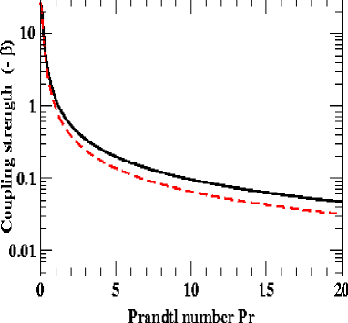
Figure 2: The coupling strength $\beta$ for rolls. Solid line from [39]. Dashed line is the dependence conjectured in [45] with the free constant chosen to match the solid line at $\mbox{\rm Pr}=0$.

The stability boundaries for infinite Prandtl number (no mean flow) are reviewed in figure 3. Hexagons exist above the thin solid line ($v=0$). The thick solid line and the dotted line are the stability boundaries for the longitudinal and transverse modes, respectively. Along the thick dashed line, rolls and hexagons have the same value of the Lyapunov functional. Hexagons become unstable to rolls ($via$ the unstable mixed mode (8)) at the thin dashed line ($u=0$). Note that since we have scaled the coefficient of the quadratic nonlinearity in (4,5) to 1, this transition occurs at $\mu=4$. For weak non-Boussinesq effects this corresponds to very small convection amplitudes. As discussed below (see also sec.4), the decomposition into transverse and longitudinal mode does not hold beyond the long-wave limit. It is replaced by a separation into a ‘wide-splitting’ and a ‘narrow-splitting’ mode [29]. The dashed-dotted line separates the regions in which the wide-splitting and the narrow-splitting mode represents the mode with maximal growth rate, respectively. In view of the effect of the mean flow it is worth noting that the regime in which the longitudinal mode is the relevant destabilizing mode is typically extremely small (below dashed-dotted line in fig.3) and it is very difficult to investigate that instability experimentally. In fact, even in numerical simulations of (4) (with $\beta=0$) we found it difficult to separate the dynamics of the two modes (see also [29]). Note that due to the scaling of the quadratic coefficient in (4,5) the usually small range over which hexagons can be observed extends from $\mu\approx 0$ to $\mu\approx 1.5$.

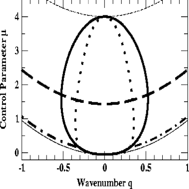
Figure 3: Summary of the stability boundaries for infinite Prandtl numbers ($\beta=0$) showing the saddle-node bifurcation (thin solid line), transition of hexagons to mixed-mode solution (thin dashed), longitudinal mode (thick solid), transverse mode (thick dotted), equal-energy line for hexagons and rolls (thick dashed), cross-over from longitudinal to transverse mode (thick dashed-dotted).

         

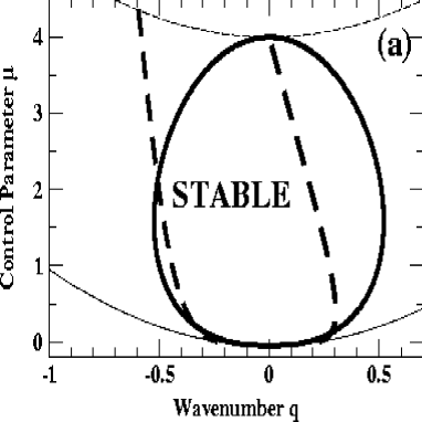
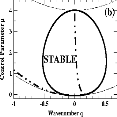
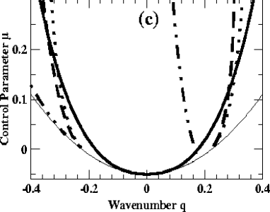
Figure 4: Stability boundaries of hexagons coupled to a two-dimensional mean flow. The thick solid line is the stability limit given by the longitudinal mode. The thick broken lines are for the transverse mode. Thin lines are as in fig.3. Panel (a) is for $\beta=-0.2$ ($\mbox{\rm Pr}\sim 5$) and panel (b) is for $\beta=-3$ ($\mbox{\rm Pr}\sim 0.5$). Panel(c): enlargement of the stability boundaries for small $\mu$ showing results for $\beta=0$, $\beta=-0.2$, and $\beta=-3$.

Figure 4a,b shows how the stability boundaries are altered by the mean flow for $\beta=-0.2$ and $\beta=-3.0$, respectively. Figure 4(c) shows an enlargement of figure 4a,b for small $\mu$. As discussed before, the mean flow affects only the transverse mode. The corresponding stability limits are denoted by thick dotted, dashed and dashed-dotted lines for $\beta=0$, $\beta=-0.2$, and $\beta=-3.0$, respectively. The thick solid line gives the stability limit due to the longitudinal mode, which is independent of $\beta$. For all values of $\beta$ it is the relevant instability immediately above the saddle-node bifurcation at which the hexagons first arise (cf. fig.4c). For somewhat larger values of $\mu$ the transverse mode becomes relevant as well. In the physically relevant case, $\beta<0$, it is destabilized by the mean flow for positive $q$ strongly reducing the stability balloon there. While for large Prandtl numbers the cross-over from the longitudinal to the transverse mode is almost imperceptible in the stability limit itself, it occurs very suddenly when the mean flow is important. This behavior has also been found in fully nonlinear stability calculations of hexagonal convection in non-Boussinesq convection [46]. For $q<0$ the transverse mode is stabilized by the mean flow. This allows the longitudinal mode to become important again for larger $\mu$. In fact, for sufficiently large $\beta$ the transverse mode does not contribute to the stability limits at low $q$ for any value of $\mu$ (cf. dashed-dotted line for $\beta=-3$ in fig.4b). Thus, for small Prandtl numbers the mean flow makes it possible to investigate the two instabilities separately. In sec.5.1 below we discuss the different nonlinear behavior arising from the two instabilities.

The leading-order phase equation (24) is isotropic. Only at higher order in the gradients this symmetry is reduced to that of the underlying hexagon pattern. Similarly, at higher orders (i.e. for larger magnitudes of the perturbation wavevector) the eigenmodes of the phase equation are not expected to be purely transverse or longitudinal any more. In sec.4 we determine the character of the destabilizing modes numerically for finite perturbation wavevectors, but only for specific values of the parameters. To obtain more general results for the influence of the mean flow on the destabilizing modes we derive here the phase equation to fifth order.

If only one of the two modes is unstable the coupled phase equations can be reduced to a single equation for the unstable mode [26]. It is obtained by eliminating the stable mode adiabatically. Since both modes are long-wave modes satisfying diffusion-like equations the elimination introduces non-local terms in the equation for the unstable mode. To demonstrate more explicitly the breaking of the isotropy and the mixing of the two modes we derive the coupled fifth-order equations for both components of the phase vector $\vec{\phi}$. This can be done systematically in the vicinity of the codimension-two point $(q^{(ct)},\mu^{(ct)})$ where both $\sigma_{l}$ and $\sigma_{t}$ are zero to cubic order (cf. (27,29)). There the orientation of the eigenmodes depends solely on the fifth-order terms. Away from the codimension-two point it is determined by the competition between the cubic and the fifth-order terms.

To facilitate the analysis we restrict to cases of weak mean flow and expand in $|\beta|\ll 1$. To cubic order, the codimension-two point is given by $q^{(ct)}=q_{0}+\beta q_{1}$ and $R_{0}^{(ct)}=R_{00}+\beta R_{01}$ with

$$q_{0}=\frac{\sqrt{2\nu+2}}{4\nu},\;\;q_{1}=\frac{3(\nu+1)}{8\nu^{3}}\;\;\mbox{and}\;\;R_{00}=\frac{1}{2\nu},\;\;R_{01}=\frac{3\sqrt{2\nu+2}}{8\nu^{3}}.$$ (30)

Here we consider the magnitude $R_{0}$ as the control parameter instead of $\mu$. To first order in $\beta$, the fifth-order, linear phase equations at the codimension-two point read as follows:

$$\partial_{t}\nabla^{2}\phi_{x} =-\frac{\nu^{2}}{8(\nu+1)}\nabla^{2}\left[(4\partial^{3}_{x}\partial_{y}+12\partial_{x}\partial^{3}_{y})\phi_{y}+(11\partial^{4}_{x}+3\partial^{4}_{y}+6\partial^{2}_{x}\partial^{2}_{y})\phi_{x}\right]$$ (31)

$$+\beta\frac{\sqrt{2(\nu+1)}}{16(\nu+1)^{2}}\left[\left(3(4+13\nu)\partial^{5}_{x}\partial_{y}+6(8+3\nu)\partial^{3}_{x}\partial^{3}_{y}+9(4+3\nu)\partial_{x}\partial^{5}_{y}\right)\phi_{y}\right.$$

$$\left.+\left(3(11+7\nu)\partial^{6}_{x}+3(17+26\nu)\partial^{4}_{x}\partial^{2}_{y}+9(3+\nu)\partial^{2}_{x}\partial^{4}_{y}+9\partial^{6}_{y}\right)\phi_{x}\right],$$

$$\partial_{t}\nabla^{2}\phi_{y} =-\frac{\nu^{2}}{8(\nu+1)}\nabla^{2}\left[(\partial^{4}_{x}+9\partial^{4}_{y}+18\partial^{2}_{x}\partial^{2}_{y})\phi_{y}+(4\partial^{3}_{x}\partial_{y}+12\partial_{x}\partial^{3}_{y})\phi_{x}\right]$$ (32)

$$+\beta\frac{\sqrt{2(\nu+1)}}{16(\nu+1)^{2}}\left[\left(3\partial^{6}_{x}+3(19+13\nu)\partial^{4}_{x}\partial^{2}_{y}+9(9+2\nu)\partial^{2}_{x}\partial^{4}_{y}+27\partial^{6}_{y}\right)\phi_{y}\right.$$

$$\left.+\left(3(4+7\nu)\partial^{5}_{x}\partial_{y}+3(8+13\nu)\partial^{3}_{x}\partial^{3}_{y}+9(4+\nu)\partial_{x}\partial^{5}_{y}\right)\phi_{x}\right].$$

A brief summary of the derivation and the full nonlinear phase equations (for $\beta=0$) are included in the appendix. Similar to the nonlinear phase equations derived in [26], eqs.(31,32) are non-local. Here, however, the reason for this is the nonlocal effect of the mean flow: for $\beta=0$ the equations become local.

         

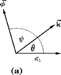
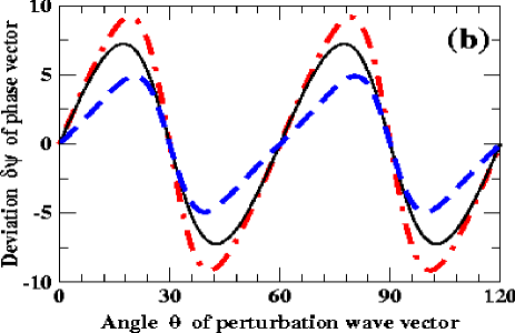
Figure 5: Panel (a): angles $\psi$ and $\theta$. Panel (b): Angle deviation $\delta\psi$ for the two eigenvectors at the codimension-two point as a function of the angle $\theta$ between $\vec{\sf k}$ and $\vec{n}_{1}$ for $\nu=2$. The thin solid line is for $\delta\psi_{0}^{(1,2)}$, and the thick dash-dotted line is $\delta\psi_{1}^{(1)}$ and the thick dashed line is $\delta\psi_{1}^{(2)}$.

The mixing between the transverse and the longitudinal modes can be quantified by the angle $\psi$ between the phase vector $\vec{\phi}$ and the wave vector $\vec{\sf k}$ of the perturbation eigenmode,

$$\psi\equiv\arctan(\frac{\hat{e}_{z}\cdot\hat{\nabla}\times\vec{\phi}}{\hat{\nabla}\cdot\vec{\phi}}).$$ (33)

Figure 5 (a) illustrates the relative positions of $\vec{\phi}$ and $\vec{\sf k}$ with respect to $\vec{n}_{1}$.

Denoting the phase angle for the pure modes by $\psi_{0}^{(1,2)}$, the pure transverse mode has $\psi_{0}^{(1)}=\pi/2$ while $\psi_{0}^{(2)}=0$ for the pure longitudinal mode. From eqs.(31,32) we find that one eigenvector, $\vec{\phi}_{1}$, is almost transverse ($\psi\sim\pi/2$) whereas the other, $\vec{\phi}_{2}$, is almost longitudinal ($\psi\sim 0$). For each mode we expand the deviation from $\psi_{0}^{(1,2)}$ in $\beta$ at the codimension-two point:

$$\delta\psi^{(1,2)}\equiv\psi^{(1,2)}-\psi_{0}^{(1,2)}=\delta\psi_{0}^{(1,2)}(\nu,\theta)+\beta\,\delta\psi_{1}^{(1,2)}(\nu,\theta)+{\cal O}(\beta^{2}),$$ (34)

where $\theta$ is the angle between ${\sf k}$ and $\hat{n}_{1}$. It turns out that in the absence of mean flow the two eigenvectors remain orthogonal to each other to fifth-order and therefore $\delta\psi_{0}^{(1)}=\delta\psi_{0}^{(2)}$. The deviation $\delta\psi_{0}^{(1,2)}$ depends very little on $\nu$. The contributions $\delta\psi_{1}^{(1,2)}$ from the mean flow decrease with increasing $\nu$ without changing sign. Fig.5 shows as an example the contributions $\delta\psi_{0,1}^{(1,2)}$ to $\delta\psi$ for $\nu=2$. The thin solid lines are $\delta\psi_{0}^{(1,2)}$ for the two eigenvectors. The thick dashed-dotted line is $\delta\psi_{1}^{(1)}$ for $\vec{\phi}_{1}$ and the thick dashed line is for $\vec{\phi}_{2}$. Note that, because $\delta\psi_{1}^{(1,2)}$ and $\delta\psi_{0}^{(1,2)}$ have the same signs and because $\beta$ is negative, the mean flow always suppresses the mixing between the two modes. Thus, the phase perturbations are closer to the pure transverse/longitudinal modes for small Prandtl number. This is also found for parameters away from the codimension-two points (see fig.6 below).

4 General Linear Stability Analysis

In this section we present results from solving the linear-stability equations (14 - 19) numerically for arbitrary perturbation wavenumbers. We first review and discuss the results for infinite Prandtl number [25, 29, 27]. The long-wave analysis of sec.3 revealed two phase instabilities associated with the longitudinal and the transverse phase mode, respectively. For finite perturbation wavenumbers these two modes become mixed and the eigenmodes of the linear stability problem are not strictly longitudinal or transverse any more. Instead they can be characterized by the angle $\theta$ between the perturbation wavevector of the fastest growing modes and $\vec{n}_{1}$. For the ‘wide-splitting’ modes $\theta=n\pi/3$, whereas for the ‘narrow-splitting’ modes $\theta=\pi/6+n\pi/3$ with $n$ an integer [29]. The terminology refers to the fact that the angle between the relevant most unstable wide-splitting modes is $2\pi/3$, whereas for the narrow-splitting modes it is only $\pi/3$ [29]. As the perturbation wavenumber goes to 0 the narrow-splitting mode turns into the longitudinal mode and the wide-splitting mode into the transverse phase mode. This is illustrated in fig.6, which shows the angle $\psi$ (eq.(33)) as a function of the angle $\theta$ between $\vec{\sf k}$ and $\vec{n}_{1}$. The thin lines refer to the case $\beta=0$ discussed here. The deviation of the destabilizing modes from these orientations increases with $|\vec{\sf k}|$ (cf. fig.5).

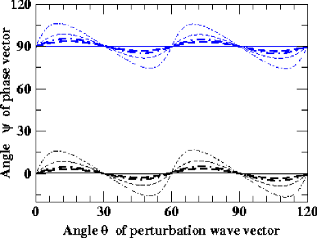
Figure 6: Angle $\psi$ (between the phase vector $\vec{\phi}$ and the perturbation wave vector $\vec{\sf k}$) as a function of the angle $\theta$ (between $\vec{\sf k}$ and $\vec{n}_{1}$) for $\mu=0.5$ and $q=0.5$. The thin lines are for coupling strength $\beta=0$, and $\beta=-0.2$ for the thick lines. The solid lines are for ${\sf k}=0$, the dashed lines for ${\sf k}=0.192$, and the dashed-dotted lines for ${\sf k}=0.224$.

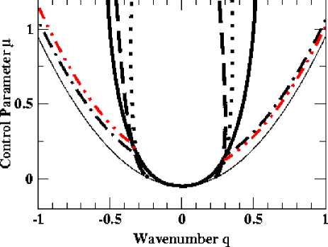
Figure 7: Cross-over from narrow-splitting to wide-splitting mode. Along the dashed-dotted (dashed-double-dotted) line the narrow- and wide-splitting modes have equal growth rates for $\beta=0$ ($\beta=-0.2$).

         

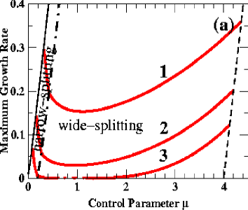
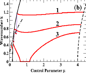
Figure 8: Results of full linear stability analysis with $\beta=0$. Panel (a): maximal growth rate as a function of $\mu$ for $q=0.6$, $0.45$ and $0.35$ (curves $1$ to $3$). Panel (b): wavenumber of the fastest growing mode for the corresponding $q$ (curves $1$ to $3$).

Numerical simulations show that the nonlinear evolution of the narrow- and of the wide-splitting modes leads to qualitatively different transient patterns with the wide-splitting mode inducing noticeably more grain boundaries between hexagon patterns of different orientation and consequently a larger number of defects than the narrow-splitting mode [29]. However, as fig.3 already suggests, the range of parameters over which the longitudinal/narrow-splitting mode dominates over the transverse/wide-splitting mode is very small and it is very difficult to separate the two modes in numerical simulations [29]. This is illustrated further in fig.7 and in fig.8. Fig.7 gives the cross-over line from the narrow-splitting to the wide-splitting mode, i.e. the line along which the growth rates of both modes are equal. Fig.8a shows the dependence of the maximal growth rate of the dominating mode as a function of the control parameter $\mu$ for three values of the wavenumber. Fig.8b shows the dependence of the wavenumber of the perturbation mode with maximal growth rate. As expected for a long-wave instability, the magnitude of the wavenumber of the fastest growing mode goes to 0 as the stability limits are reached at $\mu\approx 0.6$ and $\mu\approx 1.2$ for $q=0.35$. Although the relevant perturbation wavenumber jumps by almost a factor of 2 across the transition from the narrow-splitting to the wide-splitting mode (cf. the jump at $\mu\approx 0.4$ for $q=0.6$), it turns out that in simulations this difference is very hard to identify because the growth rates of the two modes are so similar and the narrow-splitting mode dominates only over such a small range of $\mu$.

The mean flow introduces a number of modifications in the stability behavior. The linear operator $\cal L$ becomes non-hermitian and allows complex eigenvalues. It turns out, however, that in our calculations complex eigenvalues appear only near the stability boundary of the mixed mode ($\mu=\mu_{MM}$) and beyond the long-wave stability limit given by the longitudinal mode (cf. fig.4). In numerical simulations, the transient oscillations were always accompanied by the formation of defects and an eventual transition to rolls. Possibly, the mean flow induces more relevant oscillatory instabilities in combination with nonlinear gradient terms, which also constitute non-potential terms [47, 48].

The mixing between the longitudinal and the transverse mode for finite values of ${\sf k}$ persists in the presence of mean flow. It is, however, strongly suppressed, consistent with our analytical results for the vicinity of the codimension-two point (cf. eq.(34)). This is illustrated in fig.6, where the thick lines give the angle $\psi$ of the phase vector for $\beta=-0.2$. The difference between the growth rates of the narrow- and of the wide-splitting modes is still quite small for small values of $\mu$, as it is in the case without mean flow. This is illustrated in fig.9, which shows the maximal growth rates and the associated wavenumbers for $q=+0.6$ and for $q=-0.6$ using solid and dashed lines, respectively, for different coupling strengths. For larger values of $\mu$, however, even moderate values of the coupling enhance the difference noticeably. Thus, for $\beta q<0$ the wide-splitting mode becomes much more dominant. For $\beta q>0$ the narrow-splitting mode, which in the absence of mean flow is only relevant in a very narrow range of the control parameter near the saddle-node bifurcation, becomes dominant again above a critical value of $\mu$. This reflects the asymmetry of the stability boundaries induced by the mean flow as shown in fig.4a,b. The critical value of $\mu$ decreases with decreasing Prandtl number, and below Prandtl number $\sim 2.6$ $(\beta=-0.4)$, the transverse mode is preempted by the longitudinal mode over the whole range of $\mu$. This suggests again that for sufficiently small Prandtl numbers it should be experimentally possible to study the two instability modes separately.

         

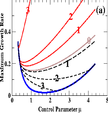
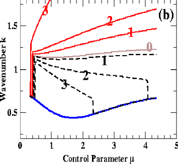
Figure 9: Results of full linear stability analysis with $q=\pm 0.6$. Solid lines are for $q=0.6$ and dashed lines are for $q=-0.6$. Panel (a): maximal growth rate as a function of $\mu$. Panel (b): wavenumber for the fastest growing mode. From curves $0$ to $3$ $\beta=0$, $-0.1$, $-0.2$, $-0.3$, respectively.

5 Numerical simulation

We now present results from numerical simulations of eqs.(4,5) using a parallel pseudo-spectral code. In sec.5.1 we compare the nonlinear evolution of the transverse and longitudinal side-band instabilities. We then discuss the impact of the mean flow on the competition between rolls and hexagons. In sec.5.2 we study the motion of penta-hepta defects in the presence of mean flow. These results shed some light on the persistence of grain boundaries in disordered hexagons patterns.

5.1 Nonlinear Evolution of the Side-band Instabilities

Transverse vs. longitudinal modes.

Without mean flow the nonlinear evolution of the two side-band instabilities of hexagon patterns has been studied numerically in some detail by Sushchik and Tsimring [29]. They find that both instabilities lead to the formation of penta-hepta defects and subsequently to disordered hexagon patterns. When only the wide-splitting perturbations are growing the emerging patterns have many grain boundaries separating domains of hexagons with different orientation. These disordered patterns persisted for a long time. When the narrow-splitting instability is dominant only few such domains appear and a regular hexagon pattern with a different wavenumber is restored within a relatively short time. Sushchik and Tsimring note that numerical simulations in the regime in which the narrow-splitting mode is the only destabilizing mode are very difficult and only present results for parameter values for which also the wide-splitting mode is destabilizing albeit to a lesser degree. These runs correspond to a quench deep into the unstable regime beyond the dashed-dotted line in fig.3 ($q=0.56$ and $\mu=0.6$). The authors associate the larger number of grain boundaries in the first case with the large angle between the components of the wide-splitting mode. A detailed comparison is difficult since no simulations are available in which only the narrow-splitting mode is active.

As discussed in sec.3 and sec.4, the mean flow couples only to the transverse/wide-splitting instability and for sufficiently small Prandtl number suppresses it completely for $\beta q>0$. This makes it possible to compare the two instabilities in detail under comparable conditions. Figs.10-12 show a comparison of the evolution of the two instabilities for $\mu=0.5$, $\nu=2$, and $\beta=-3$. The system size is $L=104$ and the numerical resolution is $256\times 256$. The wavenumbers of the initial, slightly perturbed regular hexagon patterns are chosen carefully to obtain the same linear growth rates for both modes. In particular, for $q=-0.48$ ($q=0.17$) only the longitudinal (transverse) mode is destabilizing (cf. fig.4).

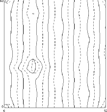
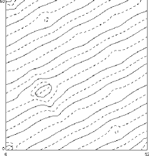
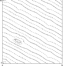
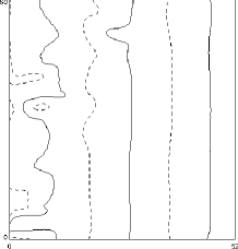
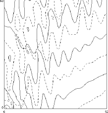
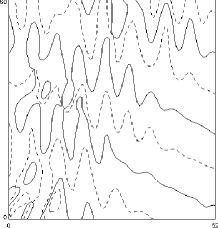
Figure 10: Zero contour lines of the amplitudes ($A_{1}$ to $A_{3}$ from left to right) for $\beta=-3$ and $\mu=0.5$. Solid lines are zero contours of the real parts, and the dashed lines are the imaginary parts. The top three panels are the longitudinal modes ($q=-0.48$) and the bottom three panels are the transverse modes ($q=0.17$) at $t=100$ in the simulations. Only a quarter of the domain is shown.

Fig.10 shows the early evolution of the instabilities in terms of the contour lines of the real and imaginary parts of the three amplitudes $A_{i}$, $i=1,2,3$. While the longitudinal mode shown in the top three panels induces compressions and dilations of the pattern, the transverse mode shears the amplitudes. Both lead to the formation of defects. However, the defects induced by the longitudinal mode are typically aligned along the rolls and form where the bulges are maximal.

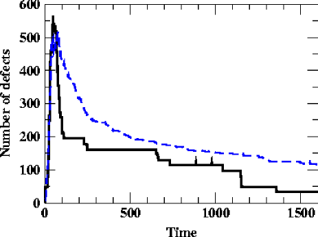
Figure 11: Number of defects as a function of time for the longitudinal case (solid line) and transverse case (dashed line).

The temporal evolution of the number of defects is shown in fig.11. For both modes, we define $t=0$ when the first defect is formed. Both modes having the same growth rate it is not surprising that in both cases the defect number grows on a similar time scale. In fact, both reach roughly the same number of defects at about the same time $t\approx 50$. In both cases the subsequent ordering of the pattern appears to occur in two stages, characterized by an initial rapid annihilation of defect pairs and a later much slower phase. In the longitudinal case the defect number decreases in large steps, which are associated with the annihilation of a string of defects roughly aligned with the rolls, whereas no such steps are visible in the transverse case. The overall decay is substantially slower for the pattern induced by the transverse instability. This had also been found in the absence of mean flow [29].

Snapshots of the reconstructed patterns at the final time $t=1750$ are shown in fig.12. Only a quarter of the whole system is shown. While in the longitudinal the defect density case is very low and the defects are essentially isolated from each other, in the transverse case most of the defects are part of grain boundaries.

         

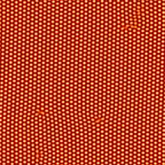
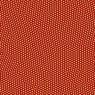
Figure 12: Reconstructed temperature for the longitudinal mode (left panel, $q=-0.48$) and the transverse mode (right panel, $q=0.17$) at $t=1750$.

To quantify the evolution of the amount of disorder in the orientation of the hexagons we determine the orientation of the local wavevector $q_{j}$ relative to the roll direction $\hat{n}_{j}$ as defined by the angle $\alpha_{j}$:

$$\alpha_{j}\equiv\arctan\left(\frac{\vec{q}_{j}\cdot\hat{\tau}_{j}}{\vec{q}_{j}\cdot\hat{n}_{j}}\right),\;\;\vec{q}_{j}\equiv\Re\left(\frac{-i\vec{\nabla}A_{j}}{A_{j}}\right)\;\;{\mbox{ for $j=1$, $2$, $3$}}.$$ (35)

In figure 13 we plot the probability distribution function (PDF) of the orientation angle $\alpha_{1}$ as a function of time for the cases shown in figures 10 and 11. Again, time $t=0$ is where the first dislocation occurs, and we have truncated the large peaks (around $\alpha_{1}=0$) at early times so that more structures can be discerned at later times. Similar PDFs are found for the other two amplitudes as well. For the longitudinal mode the PDF is centered around $\alpha_{1}=0$ from the beginning to the end, with the peak broadening around $t=0$ when the first few defects appear. Thus, for all times there is only a single domain and the hexagons remain essentially aligned with their initial orientation. In the transverse case, however, the initial peak at $\alpha_{1}=0$ quickly decays and gives way to two peaks of comparable size. This occurs around the time when the maximum number of defects is reached. The bi-modal PDF indicates that the transverse mode predominantly induces hexagons of two different orientations, which then co-exist for a long time.

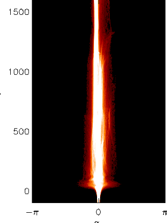
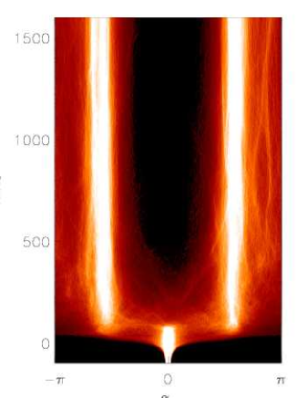
Figure 13: Evolution of the probability distribution of $\alpha_{1}$: the angle between $\vec{k}_{1}$ and $\hat{n}_{1}=\hat{x}$ for both longitudinal (left) and transverse (right).

Hexagons vs. Rolls.

In the absence of mean flow, the competition between uniform hexagons and rolls is governed by the energy difference between them. For a given $q$, hexagons are more stable than rolls for $\mu$ lower than a threshold value $\mu_{th}(q)$, at which the rolls and hexagons have the same free energy [29], while rolls are energetically favored above $\mu_{th}$. This boundary is indicated by the dashed line in figure 3. Below the dashed line, outside the stability balloon, the unstable transverse and longitudinal modes grow and evolve towards a hexagon of different wavenumber. Above this line, rolls appear during the transients and eventually replace the hexagon.

Due to the lack of a Lyapunov functional for eqs.(4,5), we resort to numerical simulations to locate the boundary between hexagon and roll in the presence of mean flow. Table 1 lists $\mu_{th}$ for $q=\pm 0.6$ for different values of $\beta$. For example, for $\beta=-0.1$ (Prandtl number $=10$) and $q=0.6$ we find rolls as the final state at $\mu=1.45$ (figure 14(a)) while a mixed state of rolls and hexagons is found at $\mu=1.425$ (figure 14(b)). Thus, the transition value in $\mu$ at $q=0.6$ for $\beta=-0.1$ is between $1.425$ and $1.45$. The enhanced instability of the transverse mode for $q=0.6$ leads apparently to an earlier transition to rolls when the Prandtl number is decreased. At this point it is not clear why the converse is not the case for $q=-0.6$.

         

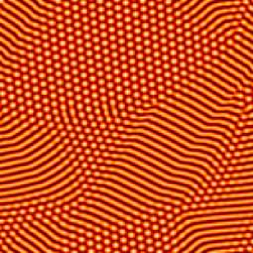
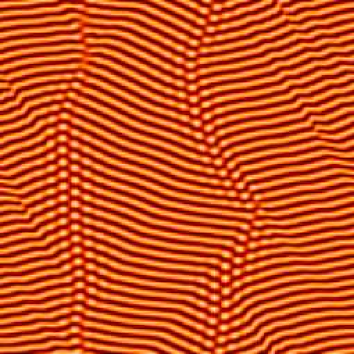
Figure 14: Reconstructed patterns from simulating equations (4,5) for $\beta=-0.1$ and $q=0.6$. On the left, $\mu=1.425$ at $t=2000$, and $\mu=1.45$ on the right panel at the same time.

$\beta$	Pr	$q=0.6$	$q=-0.6$
$0$	$\infty$	$\mu_{th}=1.5$	$\mu_{th}=1.5$
$-0.1$	$10$	$1.43$	$1.5$
$-0.2$	$5$	$1.35$	$1.5$
$-1.24$	$1$	$1.25$	$1.5$
$-3$	$0.5$	$1.1$	$1.5$

Table 1: Competition between rolls and hexagons for $q=\pm 0.6$ for different Prandtl numbers.

5.2 Effect of mean flow on motion of defects

In this section we study the effect of the mean flow on the motion of a penta-hepta defect (PHD), which is a bound state of two dislocations in two of the three amplitudes. For large Prandtl number, where the mean flow is negligible, there exists a semi-closed form solution for stationary penta-hepta defects for hexagons at the band-center ($q=0$) [33]. We study the general case with mean flow numerically by embedding two PHDs in the system as initial conditions and measure their velocity as a function of $\beta$ and $q$ for fixed $\mu=1$ and $\nu=2$.

The numerical resolution is $256\times 256$ in a system of size $L=400$ and the time step is fixed at $0.1$ for most of the results presented in this subsection. To satisfy the periodic boundary conditions, we place two PHDs of charges $(0,+1,-1)$ and $(0,-1,+1)$ in the computational domain, i.e. each PHD consists of two dislocations of opposite charges in the amplitudes $A_{2}$ and $A_{3}$. We also apply a circular ramp at $R=0.4L$, beyond which the phase is set to constant [32]. The interaction between pairs of PHD is characterized by the number $N\equiv\sum^{3}_{i=1}\delta_{j}^{1}\delta_{j}^{2}$, where $\delta_{j}^{1(2)}$ is the charge of the first (second) PHD in the $j$th amplitude [33]. In our simulations $N=-2$ and the PHDs attract each other. Their interaction decreases with distance and we find that it becomes negligible for distances larger than $300$ (for $\beta=0$ and $q=0$ the interaction-induced velocity is then below $v=0.001$). Thus in the following, we place the two PHDs at least at a distance of $300$ apart in the initial configuration for the velocity measurement of individual PHD.

In the absence of mean flow, each independent PHD is found to move at a constant velocity, which vanishes at $q=0$ [32, 33]. In the presence of mean flow, we also find that isolated defects move at a constant velocity. It is shown in figure 15 as a function of $\beta$ for $q=0$.

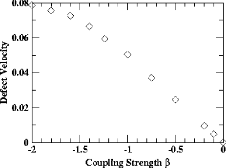
Figure 15: Defect velocity as a function of the coupling strength $\beta$ for $q=0$ and $\mu=1$. As in the case of rolls [49], for Prandtl number $\mbox{\rm Pr}\geq 0.5$ the defect speed scales as $\sim\mbox{\rm Pr}^{-1}$ (cf. fig.2).

The range of the linear scaling with respect to the coupling strength indicates that, for small $\beta$, the contribution of the mean flow to the PHD velocity is purely additive via the advective term $i\beta A(\hat{\tau}\cdot\nabla)Q$ and that the amplitudes $A_{i}$ of the defect solution are only weakly affected by the mean flow. However, as $|\beta|$ increases, the defect velocity deviates significantly from the linear scaling. This is analogous to the effect of mean flow on dislocations in roll pattern [50].

         

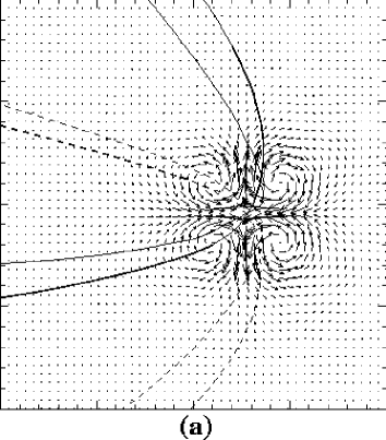
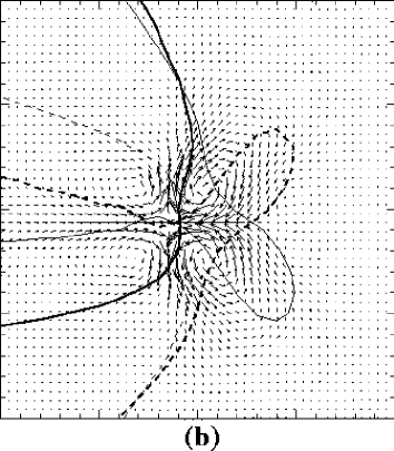
Figure 16: Mean flow structure around a PHD $(q=0)$: Panel (a) for $\beta=-0.2$ and panel(b) for $\beta=-1.4$. The solid lines (dash lines) are the zero contour lines for the real (imaginary) parts of the second amplitude are shown.

Also, for larger $|\beta|$ the mean flow structure becomes distorted near the defect as shown in figure 16. The mean flow consists of two pairs of vortices, and is almost zero away from the defect. While for $\beta=-0.2$ (left panel) the two vortex pairs are of comparable strength, the pair on the right is much stronger than that on the left when $\beta$ is decreased to $\beta=-1.4$ (right panel) This change occurs smoothly in $\beta$. When the Prandtl number is decreased further so that $\beta$ is below $-2$ the stability limit comes very close to the background wavenumber $q=0$ of the pattern and the PHD’s triggers the formation of additional defects in their vicinity.

The defect velocity also depends on the wavevectors $\vec{q}_{i}$ of the three modes making up the hexagon pattern [32]. More specifically, within equations (4,5) it depends only on the projections $\vec{q}_{i}\cdot\hat{n}_{i}$. Figure 17 shows the defect velocity as a function of $q\equiv\vec{q}_{i}\cdot\hat{n}_{i}$ for $\beta=0$ (dashed line) and $\beta=-0.2$ (solid line). The mean flow shifts the defect velocity to more positive values for all $q$, implying that the wavenumber $q_{st}$ at which the defect remains motionless is shifted from $q_{st}=0$ to negative values. For situations in which the evolution from disordered to more ordered patterns is dominated by defects this suggests that the wavenumber of the final state is in general not the critical wavenumber or that with the maximal growth rate but depends on the Prandtl number through the mean flow.

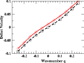
Figure 17: Defect velocity as a function of wavenumber $q$ for $\mu=1$, $\beta=0$ (dashed line) and $\beta=-0.2$ (solid line).

In various simulations of the nonlinear evolution of the instabilities of the hexagon pattern we found disordered states characterized by grain boundaries between domains of hexagons of different orientation that moved exceedingly slowly. An example of such a long-lived disordered state and the associated mean flow is shown in fig.18a,b, where the spatial structure of such long-lived grain boundaries and the corresponding mean flow is depicted for $\mu=1.2$, $q=0.6$ and $\beta=-1.24$. Here the resolution is $128\times 128$ for a system size of $L=42$.

         

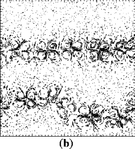
Figure 18: Panel(a): Reconstructed hexagon pattern ($q_{c}=4$) at $t\sim 14000$ for $\beta=-1.24$ (Prandtl number $\sim 1$) and $\mu=1.2$. The initial condition was an ordered, unstable hexagon pattern with $q=0.60$. Panel(b): Mean flow of the state shown in (a).

To identify the origin of these slow dynamics we performed simulations starting from patterns with two straight grain boundaries separating two hexagon patterns of different orientation rotated by $\pi/2$ relative to each other. For certain magnitudes of the initial wavevectors the grain boundaries did not annihilate each other but persisted for an exceedingly long time. Fig.19a shows such an initial condition with $\vec{q}_{2}=0.2$. A contour plot of the histogram of the local wavevector of each of the three modes in the initial condition fig.19a is shown in 20a. Solid lines pertain to $q_{1}$, dashed lines to $q_{2}$, and dashed-dotted lines to $q_{3}$. Despite the large magnitude of the reduced wavevector in the center domain the pattern is still linearly stable since the longitudinal component of the wavevector vanishes, $\vec{q}_{j}\cdot\hat{n}_{j}=0$. Within (4,5) only this projection enters the stability conditions. Either without ($\beta=0$) and with ($\beta=-2$) mean flow the initial condition evolves to the patterns shown in figs.19b and c, respectively, for $t=80,000$ and $\mu=0.5$. For $\beta=0$ simulation beyond $t=80,000$ showed little difference in the spatial structure, and the defects seem to have reached asymptotic, immobile states at the end of the simulations. In the $\beta=-2.0$ case, although the spectra and the domain sizes remain more of less the same after $t=80,000$, defects exhibit persistent lateral motion along the grain boundaries (velocity $\sim 4\times 10^{-4}$) throughout the simulation which continues beyond $t=160,000$ and lead to a slightly fluctuating shape of the domains.

     

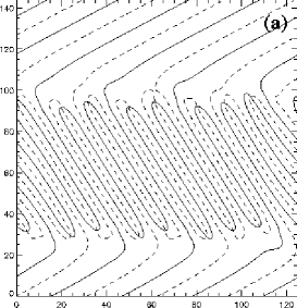
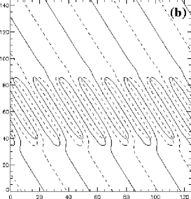
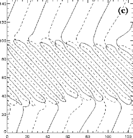
Figure 19: Zero contour lines of the real and the imaginary part of $A_{2}$. Panel (a) is for the initial conditions, and panels (b) and (c) are snapshots at $t=80000$ for $\beta=0$ and $\beta=-2.0$, respectively.

     

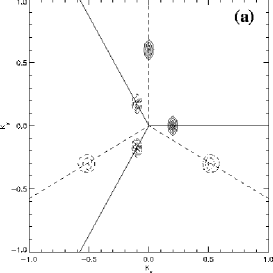
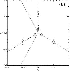
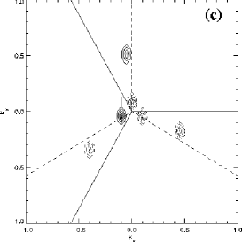
Figure 20: Wave vector spectra of the complex amplitudes shown in figure 19. Panel (a) is for the initial conditions, and panels (b) and (c) are snapshots at $t=80000$ for $\beta=0$ and $\beta=-2.0$, respectively.

The histograms of the local wavevector of the final states depicted in fig.20(b,c) show that without mean flow all three wavevectors are essentially perpendicular to $\hat{n}_{i}$ implying that individual defects would not move. In the simulation with mean flow the wavevectors are clearly not perpendicular to $\hat{n}_{i}$. Instead, $\vec{q}_{2}\cdot\hat{n}_{2}\approx-0.1$ and $\vec{q}_{3}\cdot\hat{n}_{3}\approx-0.1$. In separate simulations we find that for $\beta=-2$ and $\mu=0.5$ this is the wavenumber at which individual PHD’s do not move, $q_{st}=-0.1$. The histogram for the third wavevector $q_{1}$, however, has peaks at $(q_{x},q_{y})=(-0.1,-0.05)$ and $(-0.05,0.6)$. Thus, the two peaks have different projections onto $\hat{n}_{1}$ and only one of them agrees with $q_{st}$. This may be related to the fact that $A_{1}$ has no dislocations in the grain boundary. In separate simulations of individual PHD’s with dislocations in $A_{2}$ and $A_{3}$ we find that the velocity of the PHD depends only weakly on the wavenumber of the defect-free component ($A_{1}$), and over the whole range $-0.15<\vec{q}_{1}\cdot\hat{n}_{1}<-0.05$ the PHDs are essentially motionless. Specifically, the magnitude of the velocity is below $5\times 10^{-4}$ for $\mu=0.5$, $\beta=-2$, $\vec{q}_{2}\cdot\hat{n}_{2}=-0.1$, and $\vec{q}_{3}\cdot\hat{n}_{3}=-0.1$.

With and without mean flow, the orientation of the initial and of the final wavevectors in the top and bottom domains are different implying that in these domains the pattern rotated until the projections of their wavevectors reached $q_{st}$. This suggests that, more generally, in the ordering dynamics of hexagons starting from random initial conditions the orientation of a hexagon pattern within a given domain may rotate in a similar fashion and in the long-time dynamics the orientation of adjacent domains may predominantly be close to the stationarity condition for PHD’s, i.e. the projections of their wavevectors onto a suitably chosen $\hat{n}$ have the same value and that value is close to $q_{st}$. Of course, since our results are based on Ginzburg-Landau equations they only apply to grain boundaries across which the orientation changes only by small amounts. Furthermore, in the truncation (4,5) the higher-order transverse derivatives $\nabla\cdot\hat{\tau}_{i}$ have been neglected. They are expected to modify the stationarity condition, since the defect velocity will also depend on the transverse component of the wavevector, $\vec{q}_{i}\cdot\hat{\tau}_{i}$. The independence of the velocity on the transverse component within (4,5) is related to the isotropy of the system. Thus, it is expected that at higher orders the condition $\vec{q}_{i}\cdot\hat{n}_{i}=q_{st}$ is replaced by a more complicated, but qualitatively similar condition suggesting similar behavior for grain boundaries.

6 Conclusion

The importance of mean flows has been noted in a wide range of pattern-forming systems. Various different types can be distinguished. In systems like binary-mixture convection [51] and in surface waves on liquids with small viscosity [52] they are driven by traveling waves. In other systems they correspond to a Goldstone mode as is the case in free-slip convection (e.g. [40, 53]) or they arise from a conservation law, e.g. in systems with a deformable interface [54, 55]. Then they constitute a separate dynamical variable and satisfy an evolution equation of their own. Depending on the symmetries of the system, the additional degree of freedom can introduce a host of new phenomena (e.g. [56, 57, 58]). In this paper we have studied the mean flow that is driven in Rayleigh-Bénard convection by deformations of the convection pattern, which becomes relevant even close to onset for fluids with low Prandtl number [5, 39, 40]. In the realistic case of no-slip boundary conditions it does not constitute an additional dynamical variable. Due to the incompressibility of the fluid it can only arise in three-dimensional systems, i.e. in two-dimensionally extended patterns, and introduces then a non-local interaction. Experimentally, its most striking signatures are the skew-varicose instability and the appearance of spiral defect chaos. The experimental observation of the skew-varicose instability and of transients of spiral-defect chaos in standing waves in vertically vibrated granular media [22, 23] suggests that a similar mean flow may also be relevant in that system.

The focus of our weakly nonlinear analysis has been the impact of the mean flow on the stability and dynamics of hexagonal patterns. We have extended the usual three coupled Ginzburg-Landau equations for the description of hexagonal patterns by an equation for a vertical-vorticity mode in direct extension of previous work on roll convection at small Prandtl numbers [39, 40].

In general, there are two side-band instabilities that limit the band of stable wavenumbers of hexagons. In the absence of mean flow it is always the longitudinal long-wave mode that is the relevant destabilizing mode immediately above the saddle-node bifurcation at which the hexagons come first into existence, while the transverse long-wave mode is the relevant mode for larger amplitudes. The Rayleigh number for the cross-over from one to the other mode depends on the cross-coupling coefficient $\nu$, but for realistic value it always occurs very close to the saddle-node bifurcation. The longitudinal mode is therefore poorly accessible in the absence of mean flow (e.g. [29]). We found that in the long-wave limit only one of the two phase modes, the transverse mode, couples to the mean flow and consequently only its stability limit depends on the Prandtl number. Specifically, for sufficiently small Prandtl numbers ($\sim 2.6$ for $\nu=2$) the transverse mode is stabilized for wavenumbers below the critical wavenumber to the extent that it is preempted by the longitudinal mode over the whole range of Rayleigh numbers from the saddle-node bifurcation to the transition to the mixed mode. In this regime studies of the difference between the two modes should be accessible in experiments since the type of instability encountered depends on whether the stability limits are crossed at the low- or the high-$q$ side of the stability balloon.

Our simulations of the nonlinear evolution of the instabilities indicate that, compared to the longitudinal instability, the transverse instability leads to a considerably larger number of penta-hepta defects and to more grain boundaries separating patches of hexagons that are rotated with respect to each other. While indications of this were also found in the absence of the mean flow [29], the mean flow makes the distinction clear enough to make it worth addressing experimentally. To do so, hexagon patterns with a wavenumber away from the band center need to be initiated. Recently it has been shown that such initial conditions can, in fact, be prepared by a suitable localized heating of the fluid [37, 50]. Given the striking difference in the transients arising from the instabilities of the two modes it would be interesting to bring these techniques to bear in this system.

Although the coupling to the mean flow makes the system non-variational no regime has been identified in which oscillatory instabilities are relevant. We also find that the stability limits are always determined by long-wave instabilities and no additional instabilities at finite wavenumbers arise. Furthermore, to the order considered, the coupling to the mean flow vanishes at the band center. This implies that the pattern is always linearly stable there.

As is the case in roll convection, the mean flow also affects the motion of defects. For the penta-hepta defects relevant in hexagonal patterns we find that similar to the case of rolls the wavenumber at which the defect is stationary is shifted to wavenumbers smaller than the critical one. For coarsening experiments starting from random initial conditions one may therefore expect that the eventual wavenumber of the ordered pattern may be reduced correspondingly. Our simulation suggest that the dependence of the defect velocity on the wave vector allows one to predict which grain boundaries have a particularly long life time. Furthermore, a persistent drift of the defects in the grain boundary is also observed in the simulations. One may also expect that similar to the case of dislocations in roll patterns [38] the mean flow may allow two penta-hepta defects to form stable pairs if the background wavenumber is between the critical wavenumber and that corresponding to stationary defects.

We gratefully acknowledge useful discussions with G. Ahlers, E. Bodenschatz, B. Echebarria, D. Egolf and S. Venkataramani. This work is supported by NASA (NAG3-2113) and the Engineering Research Program of the Office of Basic Energy Sciences at the Department of Energy (DE-FG02-92ER14303). YY acknowledges computation support from the Argonne National Labs and the DOE-funded ASCI/FLASH Center at the University of Chicago.

Appendix A Derivation of the nonlinear phase equations

Here we derive the nonlinear phase equations at the codimension-two point $(q^{(ct)},R^{(ct)})$ where both $\sigma_{t}$ and $\sigma_{l}$ are zero. Mainly, to obtain explicit expressions for $(q^{(ct)},R^{(ct)})$ we consider weak mean flow, $\beta\ll 1$. (cf. eq.(30)). We rescale $X=\delta x$, $Y=\delta y$, and $T=\delta^{4}t$. In this expansion $\delta$ and $\beta$ are two independent small parameters. Here we expand the amplitudes $A_{j}=r_{j}e^{iq\hat{n}_{j}\cdot(x,y)+i\phi_{j}}$ as

$$r_{j} = R^{(ct)}_{0}+\delta^{2}r_{j2}+\delta^{4}r_{j4}+\cdots,$$ (36)

$$\phi_{j} = \delta(\phi_{j0}+\delta^{2}\phi_{j2}+\delta^{4}\phi_{j4}+\cdots),\;\;\;j=1,\;2,\;3,$$ (37)

with $R^{(ct)}_{0}$ given in eq.(30). The mean flow amplitude $Q$ is expanded accordingly in $\delta^{2}$

$$Q = \delta^{2}Q_{2}+\delta^{4}Q_{4}+\cdots.$$ (38)

We substitute the above expansions into eqs.(4,5) and solve them at successive orders for $\delta$. The mean flow feeds back to the equations for the phases $\phi_{j}$ via the amplitude modulations (cf. eq.(5)). Thus, at each order we first solve for the amplitudes and the mean flow in terms of the phases that were determined at the previous orders, and substitute these solutions into the phase equations to obtain the phases at the next order. At ${\cal O}(\delta^{2})$, up to first order in $\beta$,

$$r_{12} = -\frac{1}{\sqrt{2(1+\nu)}}\partial_{x}\phi_{x}-\frac{3}{8\nu(1+\nu)}(\partial_{x}\phi_{x}-3\partial_{y}\phi_{y})\beta,$$ (39)

$$r_{22} = -\frac{1}{4\sqrt{2(1+\nu)}}(\partial_{x}-\sqrt{3}\partial_{y})(\phi_{x}-\sqrt{3}\phi_{y})$$ (40)

$$+\frac{3}{8\nu(1+\nu)}\bigl{[}(2\partial_{x}+\sqrt{3}\partial_{y})\phi_{x}+\sqrt{3}\partial_{x}\phi_{y}\bigr{]}\beta,$$

$$r_{23} = -\frac{1}{4\sqrt{2(1+\nu)}}(\partial_{x}+\sqrt{3}\partial_{y})(\phi_{x}+\sqrt{3}\phi_{y})$$ (41)

$$+\frac{3}{8\nu(1+\nu)}\bigl{[}(2\partial_{x}-\sqrt{3}\partial_{y})\phi_{x}-\sqrt{3}\partial_{x}\phi_{y}\bigr{]}\beta,$$

$$Q_{2} = -\left(\frac{3}{4\nu\sqrt{2(1+\nu)}}+\frac{9(3\nu+1)}{16\nu^{3}(1+\nu)}\beta\right)(-\hat{e}_{z}\cdot\nabla\times\vec{\phi}).$$ (42)

At cubic order we recover eq.(24). In order to go on to fifth order we require that both $\sigma_{l}$ and $\sigma_{t}$ vanish (up to second order in $\beta$). As in section 3, the solutions are expressed in terms of the translation modes $\phi_{x}=-(\phi_{20}+\phi_{30})$ and $\phi_{y}=(\phi_{20}-\phi_{30})/\sqrt{3}$.

Repeating the same procedures at ${\cal O}(\delta^{4})$, we obtain $r_{j4}$. The expressions are too long to be displayed here. Also, at this order it is impossible to solve for $Q_{4}$ in closed form. We therefore take the Laplacian of the phase equations at this order and substitute $r_{j4}$ and $\nabla^{2}Q_{4}$ to obtain the nonlinear equations for $\phi_{x}$ and $\phi_{y}$ at the codimension-two point:

$$\partial_{t}\nabla^{2}\phi_{x} = {\cal L}_{x}+\mbox{NL}_{x0}+\beta\mbox{NL}_{x1},$$ (43)

$$\partial_{t}\nabla^{2}\phi_{y} = {\cal L}_{y}+\mbox{NL}_{y0}+\beta\mbox{NL}_{y1},$$ (44)

where ${\cal L}_{x}$ and ${\cal L}_{y}$ are the linear terms given on the right-hand-sides of eq.(31) and eq.(32), respectively. The nonlinear terms at zeroth order in $\beta$ for both equations, denoted as $\mbox{NL}_{x0}$ and $\mbox{NL}_{y0}$, read as follows:

$$\mbox{NL}_{x0}= -\frac{q_{0}\nu^{2}}{(1+\nu)^{2}}\nabla^{2}\Bigg{[}\partial_{x}\phi_{x}\left(\frac{33+25\nu}{2}\partial_{x}^{2}\phi_{x}+\frac{3+5\nu}{2}\partial_{y}^{2}\phi_{x}+(3+8\nu)\partial_{xy}^{2}\phi_{y}\right)+$$ (45)

$$(\partial_{y}\phi_{x}+\partial_{x}\phi_{y})\left((3+5\nu)\partial_{xy}^{2}\phi_{x}+\frac{3+5\nu}{2}\partial_{x}^{2}\phi_{y}+\frac{3(3+\nu)}{2}\partial_{y}^{2}\phi_{y}\right)+$$

$$\partial_{y}\phi_{y}\left(\frac{3(3+\nu)}{2}\partial_{y}^{2}\phi_{x}+\frac{3+11\nu}{2}\partial_{x}^{2}\phi_{x}+3(3+2\nu)\partial_{xy}^{2}\phi_{y}\right)\Bigg{]},$$

$$\mbox{NL}_{y0}= -\frac{q_{0}\nu^{2}}{(1+\nu)^{2}}\nabla^{2}\Bigg{[}\partial_{x}\phi_{x}\left(\frac{3+8\nu}{2}\partial_{xy}^{2}\phi_{x}+\frac{3+5\nu}{2}\partial_{x}^{2}\phi_{Y}+\frac{9(1+\nu)}{2}\partial_{y}^{2}\phi_{y}\right)+$$ (46)

$$(\partial_{y}\phi_{x}+\partial_{x}\phi_{y})\left(\frac{3+5\nu}{2}\partial_{x}^{2}\phi_{x}+\frac{3(3+\nu)}{2}\partial_{y}^{2}\phi_{x}+3(3+\nu)\partial_{xy}^{2}\phi_{y}\right)+$$

$$\partial_{y}\phi_{y}\left(3(3+2\nu))\partial_{xy}^{2}\phi_{x}+\frac{3(3+\nu)}{2}\partial_{x}^{2}\phi_{y}+\frac{27(1+\nu)}{2}\partial_{y}^{2}\phi_{y}\right)\Bigg{]},$$

with $q_{0}$ defined in eq.(30). The expressions for $\mbox{NL}_{x1}$ and $\mbox{NL}_{y1}$ are too long to be shown here.

References

- [1] E. Bodenschatz, W. Pesch, and G. Ahlers, Ann. Rev. Fluid Mech. 32, 709 (2000).
- [2] F. H. Busse, Rep. Prog. Phys. 41, 1929 (1978).
- [3] A. Newell and J. Whitehead, J. Fluid Mech. 38, 279 (1969).
- [4] L. Segel, J. Fluid Mech. 38, 203 (1969).
- [5] E. Siggia and A. Zippelius, Phys. Rev. Lett. 47, 835 (1981).
- [6] V. Croquette, P. L. Gal, A. Pocheau, and R. Guglielmetti, Europhys. Lett. 1, 393 (1986).
- [7] A. Pocheau, V. Croquette, and P. LeGal, Phys. Rev. Lett. 55, 1094 (1985).
- [8] H. S. Greenside, M. C. Cross, and W. M. Coughran, Phys. Rev. Lett. 60, 2269 (1988).
- [9] F. Daviaud and A. Pocheau, Europhys. Lett. 9, 675 (1989).
- [10] S. Morris, E. Bodenschatz, D. Cannell, and G. Ahlers, Phys. Rev. Lett. 71, 2026 (1993).
- [11] R. Cakmur, D. Egolf, B. Plapp, and E. Bodenschatz, Phys. Rev. Lett. 79, 1853 (1997).
- [12] H. Xi, J. Gunton, and J. Vinals, Phys. Rev. Lett. 71, 2030 (1993).
- [13] M. Bestehorn, M. Fantz, R. Friedrich, and H. Haken, Phys. Lett. A 174, 48 (1993).
- [14] W. Decker, W. Pesch, and A. Weber, Phys. Rev. Lett. 73, 648 (1994).
- [15] J. Liu and G. Ahlers, Phys. Rev. Lett. 77, 3126 (1996).
- [16] E. Bodenschatz, J. R. deBruyn, G. Ahlers, and D. Cannell, Phys. Rev. Lett. 67, 3078 (1991).
- [17] M. Schatz et al., Phys. Rev. Lett. 75, 1938 (1995).
- [18] Q. Ouyang and H. Swinney, Nature 352 (1991) 610 .
- [19] B. Caroli, C. Caroli, and B. Roulet, J. Crystal Growth 68, 677 (1987).
- [20] W. Edwards and S. Fauve, J. Fluid Mech. 278, 123 (1994).
- [21] F. Melo, P. Umbanhowar, and H. Swinney, Phys. Rev. Lett. 75, 3838 (1995).
- [22] J. R. deBruyn et al., Phys. Rev. Lett. 81, 1421 (1998).
- [23] J. R. de Bruyn, B. C. Lewis, M. D. Shattuck, and H. L. Swinney, Phys. Rev. E 6304, 1305 (2001).
- [24] H. Riecke, Europhys. Lett. 11, 213 (1990).
- [25] J. Lauzeral, S. Metens, and D. Walgraef, Europhys. Lett. 24, 707 (1993).
- [26] R. Hoyle, Appl. Math. Lett. 8, 81 (1995).
- [27] B. Echebarria and C. Pérez-García, Europhys. Lett. (1998).
- [28] R. Hoyle, Phys. Rev. E 61, 2506 (2000).
- [29] M. Sushchik and L. Tsimring, Physica D 74, 90 (1994).
- [30] L. Pismen and A. Nepomnyashchy, Europhys. Lett. 24, 461 (1993).
- [31] M. Rabinovich and L. Tsimring, Phys. Rev. E 49, 35 (1994).
- [32] L. Tsimring, Phys. Rev. Lett. 74, 4201 (1995).
- [33] L. Tsimring, Physica D 89, 368 (1996).
- [34] M. Bestehorn, Phys. Rev. E 48, 3622 (1993).
- [35] M. Dominguez-Lerma, D. Cannell, and G. Ahlers, Phys. Rev. A 34, 4956 (1986).
- [36] H. Riecke and H.-G. Paap, Phys. Rev. A 33, 547 (1986).
- [37] M. Schatz, priv. comm. .
- [38] E. Bodenschatz, priv. comm. .
- [39] W. Decker and W. Pesch, J. Phys II (Paris) 4, 419 (1994).
- [40] A. Bernoff, Euro. J. Appl. Math. 5, 267 (1994).
- [41] T. Callahan and E. Knobloch, Phys. Rev. E (2001).
- [42] B. Echebarria and H. Riecke, Physica D (to appear).
- [43] F. H. Busse, J. Fluid Mech. 30, 625 (1967).
- [44] B. Echebarria and H. Riecke, Physica D 139, 97 (2000).
- [45] A. Zippelius and E. D. Siggia, Phys. Rev. A 26, 1788 (1982).
- [46] V. Moroz, W. Pesch, and H. Riecke, unpublished .
- [47] H. Brand, Prog. Theor. Phys. Suppl. 99, 442 (1989).
- [48] A. Nuz et al., Physica D 135, 233 (2000).
- [49] J. A. Whitehead, J. Fluid Mech. 75, 715 (1976).
- [50] E. Bodenschatz and W. Pesch, priv. comm. .
- [51] T. Clune and E. Knobloch, Physica D 61, 106 (1992).
- [52] J. M. Vega, E. Knobloch, and C. Martel, Physica D 154, 313 (2001).
- [53] P. C. Matthews and S. M. Cox, Phys. Rev. E 62, 1473 (2000).
- [54] A. Golovin, A. Nepomnyashchy, and L. Pismen, Physica D 81, 117 (1995).
- [55] M. Renardy and Y. Renardy, Phys. Fluids 5, 2738 (1993).
- [56] P. Matthews and S. Cox, Nonlinearity 13, 1293 (2000).
- [57] A. Roxin and H. Riecke, Physica D 156, 19 (2001).
- [58] H. Riecke and G. D. Granzow, Phys. Rev. Lett. 81, 333 (1998).