Two-loop self-energy correction in H-like ions

Abstract

A part of the two-loop self-energy correction, the so-called P term, is evaluated numerically for the $1s$ state to all orders in $Z\alpha$. Our calculation, combined with the previous investigation [S. Mallampalli and J. Sapirstein, Phys. Rev. A 57, 1548 (1998)], yields the total answer for the two-loop self-energy correction in H-like uranium and bismuth. As a result, the major uncertainty is eliminated from the theoretical prediction for the Lamb shift in these systems. The total value of the ground-state Lamb shift in H-like uranium is found to be 463.93(50) eV.

PACS number(s): 31.30.Jv, 31.10.+z

Introduction

The calculation of all two-loop QED diagrams for the Lamb shift of H-like ions is one of the most challenging problems in bound-state QED. The experimental accuracy of 1 eV aimed at in measurements of the ground-state Lamb shift in H-like uranium [1] requires a calculation of the complete set of QED corrections of the order $\alpha^{2}$ without any expansion in the parameter $Z\alpha$ ($Z$ is the nuclear charge number, $\alpha$ is the fine structure constant). In high-$Z$ Li-like ions, these diagrams are the source of the major theoretical uncertainty for the $2p_{1/2}$-$2s$ transition energy [2] and, therefore, the limiting factor in comparison of theory and experiment. Also in the low-$Z$ region, the two-loop Lamb shift is important from the experimental point of view [3]. What is more, its $Z\alpha$ expansion exhibits a rather peculiar behavior, with a very slow convergence even in case of hydrogen [3]. In order to eliminate the uncertainty due to higher-order contributions, it is important to perform a non-perturbative (in $Z\alpha$) calculation of two-loop corrections even in the low-$Z$ region.

The most problematic part of the one-electron $\alpha^{2}$ contribution is the two-loop self-energy correction, represented diagramatically in Fig. 1. The diagram in Fig. 1(a) is usually divided into two parts, which are referred to as the irreducible and the reducible contribution. (The reducible contribution is defined as a part of this diagram in which intermediate states in the spectral decomposition of the middle electron propagator coincide with the initial state.) The irreducible contribution (also referred to as the loop-after-loop correction) can be shown to be gauge invariant when covariant gauges are used. Its evaluation is not very cumbersome and was accomplished in several independent investigations [4, 5, 6].

The reducible part of the diagram in Fig. 1(a) should be evaluated together with the remaining two diagrams in Fig. 1. This calculation is by far more difficult. The first attempt to attack this problem was performed by Mallampalli and Sapirstein [7]. In that work, the contribution of interest was rearranged into three parts (referred to by the authors as the M, P, and F terms), only two of which were actually evaluated. The remaining part (the P term) was left out since a new numerical technique had to be developed for its computation. In our present investigation, we perform the numerical evaluation of the missing part of the two-loop self-energy, the P term. Results of our evaluation, added to those from Ref. [7], yield the final answer for the total two-loop self-energy correction for H-like uranium and bismuth. This result disagrees with the resent calculation of the total contribution reported by Goidenko et al. [8], which is based on the partial-wave renormalization approach.

The plan of the paper is the following. The basic formulas needed for the evaluation of the P term are given in the first section, alongside with the discussion of the treatment of ultraviolet and infrared divergences. In the next section we formulate the scheme of the numerical evaluation and give some technical details. Numerical results are discussed in the last section. In that section we also collect all second-order contributions to the ground-state Lamb shift of H-like uranium and to the $2p_{1/2}$-$2s$ transition energy in Li-like uranium. In the latter case, the two-loop self-energy contribution is estimated by scaling the $1s$ result.

In this paper, we use the relativistic units ($\hbar=c=m=1$). The roman style (${\rm p}$) is used for four vectors, bold face (${\bf p}$) for three vectors and italic style ($p$) for scalars. Four vectors have the form ${\rm p}\equiv({\rm p}_{0},{\bf p})$. The scalar product of two four vectors is $({\rm p}\cdot{\rm k})={\rm p}_{0}{\rm k}_{0}-({\bf p}\cdot{\bf k})$. We use the notations ${\rm p}\!\!\!/={\rm p}_{\mu}\gamma^{\mu}$, $\hat{{\bf p}}={\bf p}/|{\bf p}|.$

I Basic formalism

In this paper we are concerned with the evaluation of the correction

$$\Delta E=\Delta E^{N1}+\Delta E^{N2}+2\Delta E^{O1}\ ,$$ (1)

where the contributions $\Delta E^{N1}$, $\Delta E^{N2}$, and $\Delta E^{O1}$ are represented by Feynman diagrams shown in Figs. 2, 3, and 4, respectively. Our consideration of these three sets of Feynman diagrams should be considered as an investigation, complementary to Ref. [7], to which we refer hereafter as I. In our calculation we use the Feynman gauge and the point nuclear model, the same as in I. Our results, combined with those from I, should yield the complete answer for the two-loop self-energy correction.

All the contribution $\Delta E^{N1}$, $\Delta E^{N2}$, and $\Delta E^{O1}$ are ultraviolet (UV) divergent. Following I, we refer to their UV-finite part as the “P term”. We note that subtractions in these contributions are chosen in such a way that each of them is free from overlapping divergences. The main problem in the evaluation of these diagrams is that they contain bound electron propagators as well as UV divergences. While UV divergences are normally separated in momentum space, the Dirac-Coulomb Green function is generally treated in the coordinate representation. The most direct way for the calculation of the P term consists in developing a numerical scheme for the evaluation of the Dirac Coulomb Green function in momentum space, which is one of the aims of the present work.

The nested contributions, $\Delta E^{N1}$ and $\Delta E^{N2}$, possess in addition some infrared (IR) divergences, which are associated with the so-called reference-state singularities. These divergences are cancelled out when considered together with the corresponding parts of the reducible contribution of the diagram in Fig. 1(a). Following I, we handle the IR divergences by introducing a regulator. This makes clear that great care should be taken in order to separate all divergences exactly in the same way as in I, in order not to miss a finite contribution.

A One-loop self-energy

We start with some basic formulas for the first-order self-energy correction. The formal expression for the unrenormalized first-order self-energy matrix element in the Feynman gauge is given by

$$\Delta E^{(1)}_{\rm unren} = \frac{i\alpha}{2\pi}\int^{\infty}_{-\infty}d\omega\int d{\bf x}_{1}d{\bf x}_{2}\,\psi^{{\dagger}}_{a}({\bf x}_{1})\alpha_{\mu}G(\varepsilon_{a}-\omega,{\bf x}_{1},{\bf x}_{2})\alpha^{\mu}\psi_{a}({\bf x}_{2})\frac{\exp(i|\omega|x_{12})}{x_{12}}\ ,$$ (2)

where ${\alpha}^{\mu}=(1,{\mbox{\boldmath$\alpha$}})$ are the Dirac matrices, and $G$ is the Dirac-Coulomb Green function,

$$G(\varepsilon,{\bf x}_{1},{\bf x}_{2})=\sum_{n}\frac{\psi_{n}({\bf x}_{1})\psi^{{\dagger}}_{n}({\bf x}_{2})}{\varepsilon-\varepsilon_{n}(1-i0)}\ .$$ (3)

Eq. (2) is written completely in coordinate space. We will need also the corresponding expression in the mixed momentum-coordinate representation. This can be obtained by the Fourier transformation of Eq. (2) over one of the radial variables,

$$\Delta E^{(1)}_{\rm unren} = -\frac{i\alpha}{2\pi}\int^{\infty}_{-\infty}d\omega\int\frac{d{\bf p}_{1}}{(2\pi)^{3}}\frac{d{\bf p}_{2}}{(2\pi)^{3}}\sum_{n}\frac{A_{\mu}^{an}(\omega,{\bf q})\psi_{n}^{{\dagger}}({\bf p}_{1})\alpha^{\mu}\psi_{a}({\bf p}_{2})}{\varepsilon_{a}-\omega-\varepsilon_{n}(1-i0)}\ ,$$ (4)

$$A_{\mu}^{an}(\omega,{\bf q}) = \frac{4\pi}{\omega^{2}-{\bf q}^{2}+i0}\int d{\bf x}\,\psi_{a}^{{\dagger}}({\bf x})\alpha_{\mu}\psi_{n}({\bf x})e^{-i{\bf q}{\bf x}}\ ,$$ (5)

where ${\bf q}={\bf p}_{1}-{\bf p}_{2}$, and

$$\psi({\bf p})=\int d{\bf x}\,e^{-i{\bf p}{\bf x}}\psi({\bf x})\ .$$ (6)

We note that while the integration over $\omega$ in Eq. (4) can be carried out by Cauchy’s theorem, we prefer to keep it, having in mind future generalizations to the two-loop case.

The renormalization of the one-loop self-energy is well known. In our work, we employ the method based on the expansion of the bound electron propagator in Eq. (2) in terms of the interaction with the nuclear Coulomb field [9]. For the detailed description of our renormalization procedure we refer the reader to [10]. The renormalized self-energy correction is represented by the sum of three finite terms,

$$\Delta E_{\rm ren}^{(1)}=\Delta E^{(1)}_{\rm zero}+\Delta E^{(1)}_{\rm one}+\Delta E^{(1)}_{\rm many}\ ,$$ (7)

where

$$\Delta E_{\rm zero}^{(1)}=\int\frac{d{\bf p}}{(2\pi)^{3}}\,\psi^{{\dagger}}_{a}({\bf p})\gamma_{0}\Sigma^{(0)}_{R}(\varepsilon_{a},{\bf p})\psi_{a}({\bf p})\ ,$$ (8)

$$\Delta E_{\rm one}^{(1)}=\int\frac{d{\bf p}_{1}}{(2\pi)^{3}}\frac{d{\bf p}_{2}}{(2\pi)^{3}}\,\psi^{{\dagger}}_{a}({\bf p}_{1})\gamma_{0}\Gamma^{0}_{R}(\varepsilon_{a},{\bf p}_{1};\varepsilon_{a},{\bf p}_{2})V_{C}({\bf q})\psi_{a}({\bf p}_{2})\ ,$$ (9)

where $V_{C}({\bf q})=-4\pi\alpha Z/|{\bf q}|^{2}$, and $\Sigma^{(0)}_{R}({\rm p})$ and $\Gamma^{\mu}_{R}({\rm p}_{1},{\rm p}_{2})$ are the renormalized free self-energy and vertex operators introduced in Appendix A. The expression for $\Delta E^{(1)}_{\rm many}$ is given by Eq. (2), where the Green function $G(\varepsilon_{a}-\omega,{\bf x}_{1},{\bf x}_{2})$ is replaced with $G^{(2+)}(\varepsilon_{a}-\omega,{\bf x}_{1},{\bf x}_{2})$,

$$G^{(2+)}(\varepsilon,{\bf x}_{1},{\bf x}_{2})=G(\varepsilon,{\bf x}_{1},{\bf x}_{2})-G^{(0)}(\varepsilon,{\bf x}_{1},{\bf x}_{2})-G^{(1)}(\varepsilon,{\bf x}_{1},{\bf x}_{2})\ ,$$ (10)

$G^{(0)}(\varepsilon,{\bf x}_{1},{\bf x}_{2})$ is the free Dirac Green function, and

$$G^{(1)}(\varepsilon,{\bf x}_{1},{\bf x}_{2})=-\int d{\bf z}G^{(0)}(\varepsilon,{\bf x}_{1},{\bf z})\frac{\alpha Z}{|{\bf z}|}G^{(0)}(\varepsilon,{\bf z},{\bf x}_{2})\ .$$ (11)

B Basic formulas for two-loop diagrams

The formal expression for the first diagram in Fig. 2 can be obtained from Eq. (2) by the substitution $G(\varepsilon_{a}-\omega,{\bf x}_{1},{\bf x}_{2})\to{G}_{N1}(\varepsilon_{a}-\omega,{\bf x}_{1},{\bf x}_{2})\ ,$ where

$${G}_{N1}(\varepsilon,{\bf x}_{1},{\bf x}_{2}) = \int\frac{d{\bf p}}{(2\pi)^{3}}\,G(\varepsilon,{\bf x}_{1},{\bf p})\gamma_{0}\biggl{[}\Sigma^{(0)}(\varepsilon,{\bf p})-\delta m\biggr{]}G(\varepsilon,{\bf p},{\bf x}_{2})\ ,$$ (12)

$$G(\varepsilon,{\bf x}_{1},{\bf p}) = \int d{\bf x}_{2}\,e^{i{\bf p}{\bf x}_{2}}G(\varepsilon,{\bf x}_{1},{\bf x}_{2})\ ,$$ (13)

$$G(\varepsilon,{\bf p},{\bf x}_{2}) = \int d{\bf x}_{1}\,e^{-i{\bf p}{\bf x}_{1}}G(\varepsilon,{\bf x}_{1},{\bf x}_{2})\ ,$$ (14)

and $\Sigma^{(0)}({\rm p})$ is the free one-loop self-energy operator defined in Appendix A.

The expression for the first diagram in Fig. 3 is obtained from Eq. (2) by the replacement $G(\varepsilon_{a}-\omega,{\bf x}_{1},{\bf x}_{2})\to{G}_{N2}(\varepsilon_{a}-\omega,{\bf x}_{1},{\bf x}_{2})\ ,$ where

$${G}_{N2}(\varepsilon,{\bf x}_{1},{\bf x}_{2}) = \int\frac{d{\bf p}_{1}}{(2\pi)^{3}}\frac{d{\bf p}_{2}}{(2\pi)^{3}}\,G(\varepsilon,{\bf x}_{1},{\bf p}_{1})V_{C}({\bf q})\gamma_{0}\Gamma^{0}(\varepsilon,{\bf p}_{1};\varepsilon,{\bf p}_{2})G(\varepsilon,{\bf p}_{2},{\bf x}_{2})\ ,$$ (15)

where $\Gamma^{\mu}({\rm p}_{1},{\rm p}_{2})$ is the free one-loop vertex operator defined in Appendix A, and $V_{C}$ is the Coulomb potential in momentum space.

We obtain the expression for the first diagram in Fig. 4 by replacing one of the $\gamma$ matrices in Eq. (4) with the vertex operator $\Gamma$,

$$\Delta E^{O1}_{\rm unren} = -\frac{i\alpha}{2\pi}\int^{\infty}_{-\infty}d\omega\int\frac{d{\bf p}_{1}}{(2\pi)^{3}}\frac{d{\bf p}_{2}}{(2\pi)^{3}}\sum_{n}\frac{A_{\mu}^{an}(\omega,{\bf q})}{\varepsilon_{a}-\omega-\varepsilon_{n}(1-i0)}$$ (17)

$$\times\psi_{n}^{{\dagger}}({\bf p}_{1})\gamma_{0}\Gamma^{\mu}(\varepsilon_{a}-\omega,{\bf p}_{1};\varepsilon_{a},{\bf p}_{2})\psi_{a}({\bf p}_{2})\ ,$$

with $A_{\mu}^{an}(\omega,{\bf q})$ given by Eq. (5)

The expressions for the remaining diagrams in Figs. 2–4 are obtained in a similar way, by replacing the Dirac-Coulomb Green function $G$ in Eqs. (12), (15), and (17) by $G^{(0)}$ or $G^{(1)}$.

C Separation of ultraviolet divergences

In this section we isolate the UV-finite part of $\Delta E$. Following I, we refer to this contribution as the P term. Considering the renormalization of the diagrams in Fig. 2, we should keep in mind that the inner self-energy loops are always accompanied by the corresponding mass counterterms.

The renormalization of the one-loop self-energy and vertex operators is defined in Appendix A. To handle the UV divergences, we regularize them by working in $D=4-\epsilon$ dimensions. The resulting expressions are

$$\Sigma^{(0)}({\rm p})-\delta m = \tilde{B}^{(1)}({\rm p}\!\!\!/-m)+\Sigma^{(0)}_{R}({\rm p})\ ,$$ (18)

$$\Gamma^{\mu}({\rm p}_{1},{\rm p}_{2}) = \tilde{L}^{(1)}\gamma^{\mu}+\Gamma^{\mu}_{R}({\rm p}_{1},{\rm p}_{2})\ ,$$ (19)

where $\tilde{B}^{(1)}$ and $\tilde{L}^{(1)}$ are UV-divergent constants, and $\Sigma^{(0)}_{R}({\rm p})$ and $\Gamma^{\mu}_{R}({\rm p}_{1},{\rm p}_{2})$ are finite. According to the Ward identity, $\tilde{B}^{(1)}=-\tilde{L}^{(1)}$.

For the renormalization of the two-loop self-energy diagrams, we refer the reader to a (very pedagogical) description given by Fox and Yennie [11]. Applying their arguments to the diagrams in Figs. 2–4, we have

$$\Delta E^{N1}+\Delta E^{N2} = \tilde{B}^{(1)}\Delta E^{(1)}_{{\rm many},D}+\Delta E^{N1}_{P}+\Delta E^{N2}_{P}\ ,$$ (20)

$$2\Delta E^{O1} = 2\tilde{L}^{(1)}\Delta E^{(1)}_{{\rm many},D}+2\Delta E^{O1}_{P}\ ,$$ (21)

where the subscript $P$ means that the corresponding contribution is UV convergent, and the subscript $D$ of $\Delta E^{(1)}_{{\rm many},D}$ indicates that this correction should be evaluated in $D$ dimensions, keeping terms of order $\epsilon$. (These terms yield a finite contribution when multiplied by divergent renormalization constants.)

The resulting expression reads

$$\Delta E=\tilde{L}^{(1)}\Delta E^{(1)}_{{\rm many},D}+\Delta E^{N1}_{P}+\Delta E^{N2}_{P}+2\Delta E^{O1}_{P}\ .$$ (22)

Here, the correction $\Delta E^{N1}_{P}$ can be obtained from the corresponding expression for $\Delta E^{N1}$ by the replacement $\Sigma^{(0)}({\rm p})\to\Sigma^{(0)}_{R}({\rm p})$, and the corrections $\Delta E^{N2}_{P}$ and $\Delta E^{O1}_{P}$ – by the corresponding substitution $\Gamma^{\mu}({\rm p}_{1},{\rm p}_{2})\to\Gamma^{\mu}_{R}({\rm p}_{1},{\rm p}_{2})$. Since all the P-terms are UV-convergent, in their evaluation we can disregard terms of order $\epsilon$ in definition of $\Sigma^{(0)}_{R}({\rm p})$ and $\Gamma^{\mu}_{R}({\rm p}_{1},{\rm p}_{2})$. We note also that the UV-divergent part of $\Delta E$ separated in Eq. (22), exactly corresponds to that in I.

D Separation of infrared divergences

Infrared divergences occur in the corrections $\Delta E^{N1}_{P}$ and $\Delta E^{N2}_{P}$ due to so-called reference-state singularities. They arise when the energy of intermediate states in the spectral decomposition of both electron propagators in Eqs. (12), (15) coincide with the energy of the reference state $vare_{a}$. As shown, e.g., in I, the divergent terms disappear when considered together with the related contributions from the reducible part of the diagram in Fig. 1(a). However, since we are going to evaluate the contributions $\Delta E^{N1}_{P}$ and $\Delta E^{N2}_{P}$ separately, a proper regularization of the IR divergences is needed. In order to preserve the compatibility of our results with those of I, we have to employ exactly the same procedure for the regularization of the IR divergences.

Following I, we introduce in the IR-divergent parts of $\Delta E^{N1}_{P}$, $\Delta E^{N2}_{P}$ a regulator $\delta$ which modifies the location of the reference-state pole of the Green function, $\varepsilon_{a}\to\varepsilon_{a}(1+\delta)$. After that, we have for the IR-divergent part of $\Delta E^{N1}_{P}$

$$\Delta E^{N1}_{P,IR}(\delta) = \frac{i\alpha}{2\pi}\sum_{\mu_{\overline{a}}}\int^{\infty}_{-\infty}d\omega\,\frac{\langle\overline{a}|\Sigma^{(0)}_{R}(\varepsilon_{a}-\omega)|\overline{a}\rangle}{(-\varepsilon_{a}\delta-\omega+i0)^{2}}\langle a\overline{a}|\frac{1-{\mbox{\boldmath$\alpha$}}_{1}{\mbox{\boldmath$\alpha$}}_{2}}{x_{12}}e^{i|\omega|x_{12}}|\overline{a}a\rangle\ ,$$ (23)

where $\overline{a}$ denotes the electron with the energy $\varepsilon_{a}$ and the angular-momentum projection $\mu_{\overline{a}}$. In Appendix B we demonstrate that $\Sigma^{(0)}_{R}(\varepsilon_{a}-\omega)$ as a function of $\omega$ can be analytically continued to the first quadrant starting from the right half of the real $\omega$ axis, and to the third quadrant from the left half of the real $\omega$ axis. Therefore, we can perform the Wick rotation of the $\omega$ integration contour in Eq. (23),

$$\Delta E^{N1}_{P,IR}(\delta) = -\frac{\alpha}{\pi}\sum_{\mu_{\overline{a}}}\Re\int_{0}^{\infty}d\omega\,\frac{\langle\overline{a}|\Sigma^{(0)}_{R}(\varepsilon_{a}-i\omega)|\overline{a}\rangle}{(\varepsilon_{a}\delta+i\omega)^{2}}\langle a\overline{a}|\frac{1-{\mbox{\boldmath$\alpha$}}_{1}{\mbox{\boldmath$\alpha$}}_{2}}{x_{12}}e^{-\omega x_{12}}|\overline{a}a\rangle\ .$$ (24)

Let us investigate the behavior of $\Delta E^{N1}_{P,IR}$ for small values of $\delta$. Writing it in a compact form, we have

$$\Delta E^{N1}_{P,IR}(\delta) = \Re\int_{0}^{\infty}d\omega\,\frac{f(\omega)}{(\varepsilon_{a}\delta+i\omega)^{2}}$$ (25)

$$= \Re\int_{0}^{\infty}d\omega\,\frac{f(\omega)-f(0)}{(\varepsilon_{a}\delta+i\omega)^{2}}$$ (26)

$$= \Re\bigl{[}f^{\prime}(0)\bigr{]}\ln\delta+\mbox{\rm terms, regular in $\delta$}\ .$$ (27)

Taking into account that

$$\Re\left.\frac{d}{d\omega}\right|_{\omega=0}\left[\sum_{\mu_{\overline{a}}}\langle\overline{a}|\Sigma^{(0)}_{R}(\varepsilon_{a}-i\omega)|\overline{a}\rangle\langle a\overline{a}|\frac{1-{\mbox{\boldmath$\alpha$}}_{1}{\mbox{\boldmath$\alpha$}}_{2}}{x_{12}}e^{-\omega x_{12}}|\overline{a}a\rangle\right]=-\langle a|\Sigma^{(0)}_{R}(\varepsilon_{a})|a\rangle\ ,$$ (28)

we have

$$\Delta E^{N1}_{P,IR}(\delta)=\frac{\alpha}{\pi}\Delta E^{(1)}_{\rm zero}\ln\delta+\Delta E^{N1}_{P,\rm infr}+O(\delta)\ .$$ (29)

Here, we have introduced the correction $\Delta E^{N1}_{P,\rm infr}$ that does not depend on the regulator $\delta$ and can be obtained by fitting numerical results for $\Delta E^{N1}_{P,IR}(\delta)$.

An analogous evaluation for the IR-divergent part of $\Delta E^{N2}_{P}$ yields

$$\Delta E^{N2}_{P,IR}(\delta)=\frac{\alpha}{\pi}\Delta E^{(1)}_{\rm one}\ln\delta+\Delta E^{N2}_{P,\rm infr}+O(\delta)\ .$$ (30)

As can be seen, the IR-divergent parts separated in Eqs. (29) and (30) are exactly cancelled by the corresponding terms in Eqs. (50) and (55) of I.

II Numerical evaluation

A Green function in the mixed representation

The main problem of the numerical evaluation of the P terms is that they involve the Dirac-Coulomb Green function in momentum space. Until recently, there has been no convenient method for its evaluation. As was pointed out in I, new numerical tools should be developed for the calculation of the P terms.

Here we address two main features which allow us to evaluate the P terms. Firstly, we express them in a form which involves the Fourier transform of the Green function over only one radial variable [Eqs. (13) and (14)]. We refer to this as the mixed (momentum-coordinate) representation. Secondly, we develop a convenient scheme for the numerical evaluation of the Green function in the mixed representation. This scheme was proposed and tested in our previous evaluation of the irreducible part of the diagram in Fig. 1(a) (the loop-after-loop contribution) [6]. Here we describe the basic idea of this approach.

We start from the B-splines method for the Dirac equation [12]. For a fixed angular-momentum quantum number $\kappa$, it provides a finite set of radial wave functions $\left\{\varphi^{i}_{\kappa,n}(x)\right\}_{n=1}^{N}\ ,$ where the superscript $i=1,2$ indicates the upper and the lower component of the radial wave function, and $n$ numerates the wave functions in the set. The wave functions are found as a linear combination of the B-splines [13],

$$\varphi^{i}_{\kappa,n}(x)=\frac{1}{x}\sum_{l}a^{i}(\kappa,n,l)B_{l}(x)\ ,$$ (31)

where $\left\{B_{l}(x)\right\}$, $l=1,2,\ldots$ is the set of the B-splines defined on the grid $\left\{x_{l}\right\}$. Since each of $B_{l}(x)$ can be represented as a piecewise polynomial, we can build the corresponding piecewise-polynomial representation for the wave functions,

$$\varphi_{\kappa,n}^{i}(x)=\frac{1}{x}\sum_{k}c^{i}_{k}(\kappa,n,l)\,(x-x_{l})^{k}\ ,\ \ \ \ x\in\left[x_{l},x_{l+1}\right]\ .$$ (32)

Consequently, the radial Dirac-Coulomb Green function in the coordinate space, defined as

$$G^{ij}_{\kappa}(\varepsilon,x_{1},x_{2})=\sum_{n}\frac{\varphi_{\kappa,n}^{i}(x_{1})\varphi_{\kappa,n}^{j}(x_{2})}{\varepsilon-\varepsilon_{n}}\ ,$$ (33)

can be written in an analogous form,

$$G_{\kappa}^{ij}(\varepsilon,x_{1},x_{2}) = \frac{1}{x_{1}x_{2}}\sum_{k_{1}k_{2}}A^{ij}_{k_{1}k_{2}}(\varepsilon,\kappa,l_{1},l_{2})(x_{1}-x_{l_{1}})^{k_{1}}(x_{2}-x_{l_{2}})^{k_{2}}\ ,$$ (35)

$$x_{1}\in\left[x_{l_{1}},x_{l_{1}+1}\right],x_{2}\in\left[x_{l_{2}},x_{l_{2}+1}\right]\ .$$

Here, the coefficients $A^{ij}_{k_{1}k_{2}}$ are given by

$$A^{ij}_{k_{1}k_{2}}(\varepsilon,\kappa,l_{1},l_{2})=\sum_{n}\frac{c^{i}_{k_{1}}(\kappa,n,l_{1})c^{j}_{k_{2}}(\kappa,n,l_{2})}{\varepsilon-\varepsilon_{n}}\ .$$ (36)

At this point, we have built the Dirac-Coulomb Green function in the piecewise-polynomial form. This representation is very convenient for the numerical evaluation. After the coefficients $A^{ij}_{k_{1}k_{2}}$ are stored for given values of $\kappa$ and $\varepsilon$, the computation of the Green function is reduced to the evaluation of a simple polynomial over each of the radial variables. We note one additional advantage of this representation of the Green function, as compared to its closed analytical form. The Green function in the form (35) and its derivative are continuous functions of the radial arguments, while its analytic representation contains a discontinuous function $\theta(x_{1}-x_{2})$ (see, e.g., [14]).

Now we turn to the Green function in the mixed representation. The Fourier transform of the radial Green function over the second radial argument can be written as

$$G_{\kappa}^{ij}(\varepsilon,x_{1},p_{2})=4\pi s(L_{j})\int_{0}^{\infty}dx_{2}\,x_{2}^{2}\,j_{L_{j}}(p_{2}x_{2})\,G_{\kappa}^{ij}(\varepsilon,x_{1},x_{2})\ ,$$ (37)

where $L_{1,2}=|\kappa\pm 1/2|-1/2$, $s(L_{1})=1$, $s(L_{2})=-\kappa/|\kappa|$, and $j_{L}(z)$ denotes the spherical Bessel function. Introducing the Fourier-transformed basic polynomials,

$$\Pi^{ik}_{l}(p)=4\pi s(L_{i})\int_{x_{l}}^{x_{l+1}}dx\,x(x-x_{l})^{k}j_{L_{i}}(px)\ ,$$ (38)

we write the Green function in the mixed representation,

$$G_{\kappa}^{ij}(\varepsilon,x_{1},p_{2})=\frac{1}{x_{1}}\sum_{k_{1}}(x_{1}-x_{l_{1}})^{k_{1}}\sum_{l_{2}k_{2}}A^{ij}_{k_{1}k_{2}}(\varepsilon,\kappa,l_{1},l_{2})\Pi^{jk_{2}}_{l_{2}}(p_{2})\ ,\ \ \ x_{1}\in\left[x_{l_{1}},x_{l_{1}+1}\right]\ .$$ (39)

Certainly, a computation in the mixed representation is essentially more time-consuming than that in coordinate space, due to necessity to evaluate the whole set of the integrals $\Pi^{jk_{2}}_{l_{2}}(p_{2})$ for each new value of $p_{2}$. Still, in actual calculations we can perform the numerical integration over $x_{1}$ first, and the total amount of computational time can be kept very reasonable.

B Evaluation of $\Delta E^{N1}_{P}$

First, we separate the total contribution $\Delta E^{N1}_{P}$ into two pieces, the IR-divergent part $\Delta E^{N1}_{P,IR}$ given by Eq. (23), and the finite remainder $\Delta E^{N1}_{P,r}$. The expression for $\Delta E^{N1}_{P,r}$ is given by

$$\Delta E^{N1}_{P,r} = \frac{i\alpha}{2\pi}\int^{\infty}_{-\infty}d\omega\int\frac{d{\bf p}}{(2\pi)^{3}}\int d{\bf x}_{1}d{\bf x}_{2}\,\frac{\exp(i|\omega|x_{12})}{x_{12}}$$ (41)

$$\times\psi^{{\dagger}}_{a}({\bf x}_{1})\alpha_{\mu}{\cal G}_{N1}(\varepsilon_{a}-\omega,{\bf x}_{1},{\bf p},{\bf x}_{2})\alpha^{\mu}\psi_{a}({\bf x}_{2})\ ,$$

where

$${\cal G}_{N1}(\varepsilon,{\bf x}_{1},{\bf p},{\bf x}_{2}) = \ \ G(\varepsilon,{\bf x}_{1},{\bf p})\gamma_{0}\Sigma^{(0)}_{R}(\varepsilon,{\bf p})G(\varepsilon,{\bf p},{\bf x}_{2})$$ (46)

$$-G^{(0)}(\varepsilon,{\bf x}_{1},{\bf p})\gamma_{0}\Sigma^{(0)}_{R}(\varepsilon,{\bf p})G^{(0)}(\varepsilon,{\bf p},{\bf x}_{2})$$

$$-G^{(1)}(\varepsilon,{\bf x}_{1},{\bf p})\gamma_{0}\Sigma^{(0)}_{R}(\varepsilon,{\bf p})G^{(0)}(\varepsilon,{\bf p},{\bf x}_{2})$$

$$-G^{(0)}(\varepsilon,{\bf x}_{1},{\bf p})\gamma_{0}\Sigma^{(0)}_{R}(\varepsilon,{\bf p})G^{(1)}(\varepsilon,{\bf p},{\bf x}_{2})$$

$$-\sum_{\mu_{\overline{a}}}\frac{\psi_{\overline{a}}({\bf x}_{1})\psi^{{\dagger}}_{\overline{a}}({\bf p})}{\varepsilon-\varepsilon_{a}+i0}\gamma_{0}\Sigma^{(0)}_{R}(\varepsilon,{\bf p})\frac{\psi_{\overline{a}}({\bf p})\psi^{{\dagger}}_{\overline{a}}({\bf x}_{2})}{\varepsilon-\varepsilon_{a}+i0}\ .$$

The next step is to perform the Wick rotation of the $\omega$-integration contour in Eq. (41). This is very convenient for the numerical evaluation since, firstly, the Dirac Green function as well as the photon propagator are exponentially decaying functions for imaginary values of $\omega$. Secondly, by this deformation of the contour we escape most of the problems connected with poles of the electron propagators and with the analytic structure of $\Sigma^{(0)}_{R}(\varepsilon)$. The analysis given in Appendix B shows that $\Sigma^{(0)}_{R}(\varepsilon_{a}-\omega)$ as a function of real $\omega$ allows the analytical continuation to the first quadrant of the complex plane starting from the right half of the real axis, and to the third quadrant from the left half of the axis. Therefore, we can rotate the integration contour on the imaginary axis dividing $\Delta E^{N1}_{P,r}$ into two pieces, $\Delta E^{N1}_{P,\rm Im}$ corresponding to the integral along the imaginary axis, and the pole term $\Delta E^{N1}_{P,\rm pole}$ that arises from the pole of electron propagator with $\varepsilon_{n}=\varepsilon_{a}$. (At this moment, we assume that $a$ corresponds to the $1s$-state.) We have

$$\Delta E^{N1}_{P,\rm Im} = -\frac{\alpha}{\pi}\Re\int_{0}^{\infty}d\omega\int\frac{d{\bf p}}{(2\pi)^{3}}\int d{\bf x}_{1}d{\bf x}_{2}\,\frac{\exp(-\omega x_{12})}{x_{12}}$$ (48)

$$\times\psi^{{\dagger}}_{a}({\bf x}_{1})\alpha_{\mu}{\cal G}_{N1}(\varepsilon_{a}-i\omega,{\bf x}_{1},{\bf p},{\bf x}_{2})\alpha^{\mu}\psi_{a}({\bf x}_{2})\ ,$$

$$\Delta E^{N1}_{P,\rm pole} = \frac{\alpha}{2}\Re\int\frac{d{\bf p}}{(2\pi)^{3}}\int d{\bf x}_{1}d{\bf x}_{2}\,\frac{1}{x_{12}}\psi^{{\dagger}}_{a}({\bf x}_{1})\alpha_{\mu}{\cal G}_{N1}^{\rm pole}(\varepsilon_{a},{\bf x}_{1},{\bf p},{\bf x}_{2})\alpha^{\mu}\psi_{a}({\bf x}_{2})\ ,$$ (49)

where

$${\cal G}_{N1}^{\rm pole}(\varepsilon_{a},{\bf x}_{1},{\bf p},{\bf x}_{2}) = \sum_{\mu_{\overline{a}}}\Bigl{[}\psi_{\overline{a}}({\bf x}_{1})\psi^{{\dagger}}_{\overline{a}}({\bf p})\gamma_{0}\Sigma^{(0)}_{R}(\varepsilon_{a},{\bf p})G^{\rm red}(\varepsilon_{a},{\bf p},{\bf x}_{2})$$ (51)

$$+G^{\rm red}(\varepsilon_{a},{\bf x}_{1},{\bf p})\gamma_{0}\Sigma^{(0)}_{R}(\varepsilon_{a},{\bf p})\psi_{\overline{a}}({\bf p})\psi^{{\dagger}}_{\overline{a}}({\bf x}_{2})\Bigr{]}\ ,$$

and $G^{\rm red}$ is the reduced Dirac-Coulomb Green function,

$$G^{\rm red}(\varepsilon,{\bf x}_{1},{\bf x}_{2})=\sum^{\varepsilon_{n}\neq\varepsilon_{a}}_{n}\frac{\psi_{n}({\bf x}_{1})\psi^{{\dagger}}_{n}({\bf x}_{2})}{\varepsilon-\varepsilon_{n}(1-i0)}\ .$$ (52)

Finally, we collect all contributions to $\Delta E^{N1}_{P}$,

$$\Delta E^{N1}_{P}(\delta)=\frac{\alpha}{\pi}\Delta E^{(1)}_{\rm zero}\ln\delta+\Delta E^{N1}_{P,\rm infr}+\Delta E^{N1}_{P,\rm pole}+\Delta E^{N1}_{P,\rm Im}+O(\delta)\ .$$ (53)

We note that instead of dividing $\Delta E^{N1}_{P}$ into three parts, we could have introduced the regulator $\delta$ right from the beginning in $\Delta E^{N1}_{P}$, as it was done in I for the “M terms”. However, this would cause a rapidly varying structure of the integrand in the low-$\omega$ region, which makes calculations much more time-consuming. (E.g., for the pole term introducing a regulator would involve a numerical evaluation of the integral which yields the $\delta$-function in the limit $\delta\to 0$.) In our approach, on the contrary, only the IR-divergent part is evaluated with the regulator; the corresponding calculation is relatively simple and allows accurate fitting to the form (29).

Let us now outline essential features of our numerical evaluation. As can be seen, the dependence of the functions ${\cal G}_{N1}$ and ${\cal G}_{N1}^{\rm pole}$ on the angular parts of ${\bf x}_{1}$ and ${\bf x}_{2}$ is exactly the same as that of the Dirac Green function. Therefore, the angular integration causes no problems and can be performed by a straightforward generalization of formulas given in Ref. [10]. The most problematic part of the numerical evaluation of $\Delta E^{N1}_{P}$ is the calculation of $\Delta E^{N1}_{P,\rm Im}$. All numerical integrations were performed by the Gauss-Legendre quadratures. The ordering of integrations in our computation coincides with that of Eq. (48), with the summation over the angular-momentum quantum number of intermediate states $\kappa$ moved outside. For each value of $\kappa$ and $\omega$, we store three sets of complex coefficients $A^{ij}_{k_{1}k_{2}}$ corresponding to the functions $G$, $G^{(0)}$, and $G^{(1)}$. For each value of $p$, we calculate also a set of the Fourier-transformed polynomials $\Pi^{ik}_{l}(p)$. After this, the integrations over the radial variables $x_{1}$, $x_{2}$ are performed. This scheme is rather efficient and was used for the evaluation of $\Delta E^{N1}_{P,\rm Im}$. The corrections $\Delta E^{N1}_{P,\rm infr}$ and $\Delta E^{N1}_{P,\rm pole}$ were calculated in several different ways, which served as a good test for our numerical procedure.

The actual calculation was performed with the basis set constructed typically with 50-60 B-splines of order 6 and employing the point nuclear model. The cavity size of 1 a.u. was employed for $Z=80$, which was scaled as $\gamma/Z$ with $Z$, $\gamma=\sqrt{1-(\alpha Z)^{2}}$. We use an exponential grid with the first knot of about 0.001 a.u. for $Z=80$. This particular grid was chosen since it yields an optimal convergence in the evaluation of the first-order self-energy correction with respect to the number of knots. The infinite summation over the angular-momentum quantum number of intermediate states $\kappa$ was terminated typically at $|\kappa_{\rm max}|=7$. The tail of the expansion was estimated by polynomial fitting in $1/|\kappa|$. The results of the numerical evaluation of the individual contributions to $\Delta E^{N1}_{P}$ are presented in Table I for $Z=83$, $90$, and $92$. The numerical errors, quoted in the table, originate mainly from the sensitivity of the result to the number of knots and different grids.

C Evaluation of $\Delta E^{N2}_{P}$

The correction $\Delta E^{N2}_{P}$ can be written in the same way as $\Delta E^{N1}_{P}$,

$$\Delta E^{N2}_{P}(\delta)=\frac{\alpha}{\pi}\Delta E^{(1)}_{\rm one}\ln\delta+\Delta E^{N2}_{P,\rm infr}+\Delta E^{N2}_{P,\rm pole}+\Delta E^{N2}_{P,\rm Im}+O(\delta)\ .$$ (54)

Here, we again separate the IR-divergent part [Eq. (30)] and perform the Wick rotation of the $\omega$-integration contour, separating the corresponding pole contribution ($\Delta E^{N2}_{P,\rm pole}$). We note that the rotation of the contour is possible because the vertex operator $\Gamma^{\mu}(\varepsilon_{a}-\omega,\varepsilon_{a}-\omega)$ as a function of real $\omega$ allows an analytic continuation in the region of interest, as shown in Appendix C. The resulting expression reads

$$\Delta E^{N2}_{P,\rm Im} = -\frac{\alpha}{\pi}\Re\int_{0}^{\infty}d\omega\int\frac{d{\bf p}_{1}}{(2\pi)^{3}}\frac{d{\bf p}_{2}}{(2\pi)^{3}}\int d{\bf x}_{1}d{\bf x}_{2}\,\frac{\exp(-\omega x_{12})}{x_{12}}V_{C}({\bf q})$$ (56)

$$\times\psi^{{\dagger}}_{a}({\bf x}_{1})\alpha_{\mu}{\cal G}_{N2}(\varepsilon_{a}-i\omega,{\bf x}_{1},{\bf p}_{1},{\bf p}_{2},{\bf x}_{2})\alpha^{\mu}\psi_{a}({\bf x}_{2})\ ,$$

where

$${\cal G}_{N2}(\varepsilon,{\bf x}_{1},{\bf p}_{1},{\bf p}_{2},{\bf x}_{2}) = \ \ G(\varepsilon,{\bf x}_{1},{\bf p}_{1})\gamma_{0}\Gamma^{0}_{R}(\varepsilon,{\bf p}_{1};\varepsilon,{\bf p}_{2})G(\varepsilon,{\bf p}_{2},{\bf x}_{2})$$ (59)

$$-G^{(0)}(\varepsilon,{\bf x}_{1},{\bf p}_{1})\gamma_{0}\Gamma^{0}_{R}(\varepsilon,{\bf p}_{1};\varepsilon,{\bf p}_{2})G^{(0)}(\varepsilon,{\bf p}_{2},{\bf x}_{2})$$

$$-\sum_{\mu_{\overline{a}}}\frac{\psi_{\overline{a}}({\bf x}_{1})\psi^{{\dagger}}_{\overline{a}}({\bf p}_{1})}{\varepsilon-\varepsilon_{a}+i0}\gamma_{0}\Gamma^{0}_{R}(\varepsilon,{\bf p}_{1};\varepsilon,{\bf p}_{2})\frac{\psi_{\overline{a}}({\bf p}_{2})\psi^{{\dagger}}_{\overline{a}}({\bf x}_{2})}{\varepsilon-\varepsilon_{a}+i0}\ .$$

Assuming that $a$ is the $1s$ state, the pole contribution is given by

$$\Delta E^{N2}_{P,\rm pole} = \frac{\alpha}{2}\Re\int\frac{d{\bf p}_{1}}{(2\pi)^{3}}\frac{d{\bf p}_{2}}{(2\pi)^{3}}\int d{\bf x}_{1}d{\bf x}_{2}\,\frac{1}{x_{12}}V_{C}({\bf q})$$ (61)

$$\times\psi^{{\dagger}}_{a}({\bf x}_{1})\alpha_{\mu}{\cal G}_{N2}^{\rm pole}(\varepsilon_{a},{\bf x}_{1},{\bf p}_{1},{\bf p}_{2},{\bf x}_{2})\alpha^{\mu}\psi_{a}({\bf x}_{2})\ ,$$

where

$${\cal G}_{N2}^{\rm pole}(\varepsilon_{a},{\bf x}_{1},{\bf p}_{1},{\bf p}_{2},{\bf x}_{2}) = \sum_{\mu_{\overline{a}}}\Bigl{[}\psi_{\overline{a}}({\bf x}_{1})\psi^{{\dagger}}_{\overline{a}}({\bf p}_{1})\gamma_{0}\Gamma^{0}_{R}(\varepsilon_{a},{\bf p}_{1};\varepsilon_{a},{\bf p}_{2})G^{\rm red}(\varepsilon_{a},{\bf p}_{2},{\bf x}_{2})$$ (63)

$$+G^{\rm red}(\varepsilon_{a},{\bf x}_{1},{\bf p}_{1})\gamma_{0}\Gamma^{0}_{R}(\varepsilon_{a},{\bf p}_{1};\varepsilon_{a},{\bf p}_{2})\psi_{\overline{a}}({\bf p}_{2})\psi^{{\dagger}}_{\overline{a}}({\bf x}_{2})\Bigr{]}\ .$$

The angular integration in these expressions is straightforward, due to the fact that the functions ${\cal G}_{N2}$ and ${\cal G}_{N2}^{\rm pole}$ have the same dependence on the angular parts of ${\bf x}_{1}$ and ${\bf x}_{2}$ as the Dirac Green function $G$. The numerical evaluation of the correction $\Delta E^{N2}_{P,\rm Im}$ is much more time-consuming than that of $\Delta E^{N1}_{P,\rm Im}$. This is because the integration over $|{\bf p}|$ in Eq. (48) (after the angular integration has been carried out) is substituted by the triple integration over $|{\bf p}_{1}|$, $|{\bf p}_{2}|$, and $\xi=(\hat{{\bf p}}_{1}\cdot\hat{{\bf p}}_{2})$. So, the numerical evaluation of $\Delta E^{N2}_{P,\rm Im}$ involves one infinite partial-wave summation and a seven-fold numerical integration. (One additional integral comes from the evaluation of the Green function in the mixed representation.) While it is possible to evaluate $\Delta E^{N2}_{P,\rm Im}$ in a similar way as $\Delta E^{N1}_{P,\rm Im}$, we have found a more efficient method for its computation. To this end, we rewrite Eq. (56) as follows

$$\Delta E^{N2}_{P,\rm Im} = -\frac{\alpha}{\pi}\Re\int_{0}^{\infty}d\omega\int\frac{d{\bf p}_{1}}{(2\pi)^{3}}\frac{d{\bf p}_{2}}{(2\pi)^{3}}\,V_{C}({\bf q})$$ (66)

$$\times\Biggl{\{}\sum_{n_{1}n_{2}}{}^{\prime}\frac{\psi^{{\dagger}}_{n_{1}}({\bf p}_{1})\,\gamma_{0}\Gamma^{0}_{R}\,\psi_{n_{2}}({\bf p}_{2})}{(\varepsilon_{a}-i\omega-\varepsilon_{n_{1}})(\varepsilon_{a}-i\omega-\varepsilon_{n_{2}})}\langle an_{2}|\frac{1-{\mbox{\boldmath$\alpha$}}_{1}{\mbox{\boldmath$\alpha$}}_{2}}{x_{12}}e^{-\omega x_{12}}|n_{1}a\rangle$$

$$-\sum_{{\beta}{\gamma}}\frac{u^{{\dagger}}_{{\beta}}({\bf p}_{1})\,\gamma_{0}\Gamma^{0}_{R}\,u_{{\gamma}}({\bf p}_{2})}{(\varepsilon_{a}-i\omega-\varepsilon_{{\beta}})(\varepsilon_{a}-i\omega-\varepsilon_{{\gamma}})}\langle a{\gamma}|\frac{1-{\mbox{\boldmath$\alpha$}}_{1}{\mbox{\boldmath$\alpha$}}_{2}}{x_{12}}e^{-\omega x_{12}}|{\beta}a\rangle\Biggr{\}}\ ,$$

where $\Gamma^{0}_{R}\equiv\Gamma^{0}_{R}(\varepsilon_{a}-i\omega,{\bf p}_{1};\varepsilon_{a}-i\omega,{\bf p}_{2})$, $\psi_{n_{1}}$ and $\psi_{n_{2}}$ stand for solutions of the Dirac equation with the Coulomb potential, $u_{\beta}$ and $u_{\gamma}$ denote solutions of the free Dirac equation, and the prime on the sum indicates that the term with $\varepsilon_{n_{1}}=\varepsilon_{n_{2}}=\varepsilon_{a}$ is omitted. In order to evaluate Eq. (66), we introduce the matrix $S$,

$$S^{ij}_{\kappa}(\omega,p_{1},p_{2})=\sum_{n_{1}n_{2}}{}^{\prime}\frac{\varphi^{i}_{\kappa,n_{1}}(p_{1})\varphi^{j}_{\kappa,n_{2}}(p_{2})}{(\varepsilon_{a}-i\omega-\varepsilon_{n_{1}})(\varepsilon_{a}-i\omega-\varepsilon_{n_{2}})}\langle an_{2}|\frac{1-{\mbox{\boldmath$\alpha$}}_{1}{\mbox{\boldmath$\alpha$}}_{2}}{x_{12}}e^{-\omega x_{12}}|n_{1}a\rangle\ ,$$ (67)

where $\varphi^{i}(p)$ ($i=1,2$) stands for the radial components of the corresponding wave function. An analogous matrix $S^{(0)}$ is introduced also for the second part of Eq. (66). For each value of $\kappa$ and $\omega$, we calculate coefficients of the piecewise-polynomial representation of $S$, $S^{(0)}$. Then, for each values of $p_{1}$ and $p_{2}$, we store two sets of the Fourier-transformed polynomials, $\Pi^{ik}_{l}(p_{1})$ and $\Pi^{ik}_{l}(p_{2})$. Finally, the integration over $\xi$ is performed.

The results of the numerical evaluation of the individual contributions to $\Delta E^{N2}_{P}$ are presented in Table II for $Z=83$, $90$, and $92$.

D Evaluation of $\Delta E^{O1}_{P}$

The expression for $\Delta E^{O1}_{P}$ can be easily obtained from Eq. (17), after rewriting it in terms of the Green function and making the substitutions $G\to G^{(2+)}$ and $\Gamma^{\mu}\to\Gamma^{\mu}_{R}$,

$$\Delta E^{O1}_{P} = -2i\alpha\int^{\infty}_{-\infty}d\omega\int\frac{d{\bf p}_{1}}{(2\pi)^{3}}\frac{d{\bf p}_{2}}{(2\pi)^{3}}\int d{\bf z}\,\frac{\exp(-i{\bf q}{\bf z})}{\omega^{2}-{\bf q}^{2}+i0}$$ (69)

$$\times\psi_{a}^{{\dagger}}({\bf z})\alpha_{\mu}G^{(2+)}(\varepsilon_{a}-\omega,{\bf z},{\bf p}_{1})\gamma_{0}\Gamma^{\mu}_{R}(\varepsilon_{a}-\omega,{\bf p}_{1};\varepsilon_{a},{\bf p}_{2})\psi_{a}({\bf p}_{2})\ ,$$

where ${\bf q}={\bf p}_{1}-{\bf p}_{2}$, $G^{(2+)}(\varepsilon,{\bf z},{\bf p}_{1})$ is the many-potential Green function [Eq. (10)] in the momentum-coordinate representation. The analysis given in Appendix C shows that the vertex operator $\Gamma^{\mu}_{R}(\varepsilon_{a}-\omega,\varepsilon_{a})$ as a function of real $\omega$ allows the analytical continuation to the first quadrant of the complex $\omega$ plane starting from the right half of the real axis, and to the third quadrant from the left half of the axis. Therefore, we can perform the Wick rotation of the integration contour, separating the corresponding pole contribution,

$$\Delta E^{O1}_{P}=\Delta E^{O1}_{P,\rm pole}+\Delta E^{O1}_{P,\rm Im}\ .$$ (70)

The angular integration in Eq. (69) is by far more difficult as compared to the contributions considered so far. As the involved expressions are rather lengthy, we do not give their detailed consideration here. However, in order to give the reader an idea how the angular integration is performed, we note that Eq. (17) is very similar to the free-vertex contribution which is encountered in a calculation of the self-energy screening diagrams (compare with Eq. (68) in Ref. [15]). Basically, the angular integration in Eq. (69) is the same as described in detail in Ref. [15]. The only difference is that in Ref. [15] the integration was demonstrated for two particular states, $n=2p_{1/2}$ and $2s$. In Eq. (69) we need a generalization of that procedure for an arbitrary $n$, which is somewhat tedious but straightforward.

Let us discuss now the numerical evaluation of $\Delta E^{O1}_{P}$. After the angular integration is carried out, a typical contribution to $\Delta E^{O1}_{P,\rm Im}$ can be written as follows

$$t = \sum_{\kappa}\int_{0}^{\infty}d\omega\int_{0}^{\infty}dp_{1}\int_{0}^{\infty}dp_{2}\int_{-1}^{1}d\xi\int_{0}^{\infty}dz\,\frac{p_{1}^{2}\,p_{2}^{2}\,z^{2}}{\omega^{2}+q^{2}}$$ (72)

$$\times j_{l}(qz)\varphi^{i}_{a}(z)G_{\kappa}^{(2+)^{ij}}(\varepsilon_{a}-i\omega,z,p_{1})f(p_{1},p_{2},\xi)\varphi_{a}^{j}(p_{2})\ ,$$

where $p_{1}=|{\bf p}_{1}|$, $p_{2}=|{\bf p}_{2}|$, $\xi=(\hat{{\bf p}}_{1}\cdot\hat{{\bf p}}_{2})$, $q^{2}=p_{1}^{2}+p_{2}^{2}-2p_{1}p_{2}\xi$, $\varphi^{i}$ is a radial component of the wave function, $G^{(2+)^{ij}}_{\kappa}$ denotes a radial component of $G^{(2+)}$, $j_{L}$ is a spherical Bessel function, and $f(p_{1},p_{2},\xi)$ originates from the vertex operator. Eq. (72) involves one infinite partial-wave summation and a six-fold numerical integration. (The sixth integral is the momentum integration in the evaluation of the Green function in the mixed representation. Two additional integrations can be also mentioned, one over the Feynman parameter in the evaluation of $f(p_{1},p_{2},\xi)$, and another a radial integration in the computation of $G^{(1)}$. This makes the total dimension of the integral to be 8.) Two of these integrations involve spherical Bessel functions, which oscillate strongly in the high-momenta region. In order to keep the amount of computational time within an acceptable limit, the general scheme of the calculation should be chosen carefully. In our approach, we introduce the following change of variables [10]: $\left\{p_{1},p_{2},\xi\right\}\to\left\{x,y,q\right\}$, where $x=p_{1}+p_{2}$, $y=p_{>}-p_{<}$, $q^{2}=p_{1}^{2}+p_{2}^{2}-2p_{1}p_{2}\xi$, $p_{>}=\max(p_{1},p_{2})$, $p_{<}=\min(p_{1},p_{2})$. After that, we have

$$\int_{0}^{\infty}dp_{1}\int_{0}^{\infty}dp_{2}\int_{-1}^{1}d\xi\,F(p_{1},p_{2},\xi)=\int_{0}^{\infty}dx\int_{0}^{x}dy\int_{y}^{x}dq\,\frac{q}{2p_{1}p_{2}}\Bigl{[}F(p_{1},p_{2},\xi)+F(p_{2},p_{1},\xi)\Bigr{]}\ .$$ (73)

In the actual calculation, the outermost loop was the summation over $\kappa$. The next loop is the $\omega$ integration. For given values of $\kappa$ and $\omega$, we store a set of coefficients of the piecewise-polynomial representation of $G^{(2+)}_{\kappa}$. These coefficients are obtained as the difference of the corresponding coefficients for $G_{\kappa}$, $G_{\kappa}^{(0)}$, and $G^{(1)}_{\kappa}$, as stated in Eq. (11). The next two loops are the integrations over $x$ and $y$. For each value of $p_{1}$, we store a set of the Fourier-transformed polynomials $\Pi^{ik}_{l}(p_{1})$. The next step is the integration over $q$ and the evaluation of $f(p_{1},p_{2},\xi)$, which involves an integration over the Feynman parameter (see, e.g., Ref. [10]). The innermost loop is the integration over $z$. Its optimization is the most critical part from the point of view of computational time. For small values of $q$, we use Gauss-Legendre quadratures. When $q$ is large, we decompose $j_{l}(qx)$ in a combination of $\sin(qx)$ and $\cos(qx)$, and use the standard routine for the $\sin$- and $\cos$-Fourier transforms based on the generalized Clenshaw-Curtis algorithm. At that stage of the computation, both $\varphi^{i}_{a}$ and $G^{(2+)^{ij}}_{\kappa}$ are represented by piecewise polynomials and, therefore, the $z$ integration can be performed rather fast.

A good test for our numerical procedure is to evaluate the many-potential part of the first-oder self-energy correction, which can be obtained from Eq. (69) by the substitution $\Gamma^{\mu}_{R}\to\gamma^{\mu}$.

The results of the numerical calculation of the individual contributions to $\Delta E^{O1}_{P}$ are presented in Table III for $Z=83$, $90$, and $92$.

III Results and discussion

In this paper we present the numerical evaluation of the correction $\Delta E$, given by the three sets of diagrams which are shown in Figs. 2–4. Putting together Eqs. (1), (22), (53), (54), and (70), we have

$$\Delta E = \tilde{L}^{(1)}\Delta E^{(1)}_{{\rm many},D}+\frac{\alpha}{\pi}\biggl{[}\Delta E^{(1)}_{\rm zero}+\Delta E^{(1)}_{\rm one}\biggr{]}\ln\delta$$ (77)

$$+\Delta E^{N1}_{P,\rm infr}+\Delta E^{N1}_{P,\rm pole}+\Delta E^{N1}_{P,\rm Im}$$

$$+\Delta E^{N2}_{P,\rm infr}+\Delta E^{N2}_{P,\rm pole}+\Delta E^{N2}_{P,\rm Im}$$

$$+2\Delta E^{O1}_{P,\rm pole}+2\Delta E^{O1}_{P,\rm Im}+O(\delta)\ .$$

The UV-finite difference $\Delta E-\tilde{L}^{(1)}\Delta E^{(1)}_{{\rm many},D}$ corresponds to what in I is called the P term. The IR-divergent contributions, still presented in the P term, are cancelled when considered together with Eqs. (50) and (55) of I. When all $\delta$-dependent terms are put together, the limit $\delta\to 0$ can be taken, and contributions of order $\delta$ and higher vanish. Finite individual contributions to $\Delta E^{N1}_{P}$, $\Delta E^{N2}_{P}$, and $\Delta E^{O1}_{P}$ are listed in Tables I–III, respectively. In Table IV we collect all finite contributions to $\Delta E$.

Now we can obtain a finite, gauge-independent (within the covariant gauges) result for the sum of the diagrams in Figs. 1(b,c) and the reducible part of the diagram in Fig. 1(a). In order to get this, we should add together the contributions listed in Table IV, the results from I for the M terms (Eqs. (50), (52), and (55) of I) and those for the F terms (Table IV of I). This yields $-$0.903(11) eV for the ground state of H-like uranium and $-$0.575(11) eV for bismuth. Adding this to the irreducible part of the diagram in Fig. 1(a) ($-$0.971 eV for $Z=92$ [4, 5] and $-$0.544 eV for $Z=83$, this work), we have for the total two-loop self-energy correction, given by the diagrams in Fig. 1, $-$1.874(11) eV for $Z=92$ and $-$1.119(11) eV for $Z=83$.

The numerical results for the sum of the diagrams in Figs. 1(b,c) and the reducible part of the diagram in Fig. 1(a), obtained by combining the present calculation with that of I, can be compared with the recent evaluation announced in Ref. [8]. The results of $-$0.903(11) eV ($Z=92$) and $-$0.575(11) eV ($Z=83$) obtained in this work should be compared with 1.28(15) eV and 0.73(9) eV, respectively, reported in Ref. [8]. Surprisingly enough, the comparison shows that the results disagree even with respect to the overall sign of the contribution. Commenting this disagreement, one can mention that the partial-wave renormalization procedure, used in Ref. [8], is known to produce certain spurious terms due to the noncovariant nature of the regularization (see Ref. [16] and a discussion given in Refs. [17, 6]). We also note that some assumptions employed in the numerical evaluation of Ref. [8] make it difficult to keep accuracy under proper control in the computation. Still, in order to resolve this disagreement, it is desirable to perform an evaluation of the total two-loop self-energy correction within the covariant approach from the beginning up to the end by the same authors. This will be the aim of our future investigation.

With this evaluation of the two-loop self-energy correction, we complete the long-lasting problem of calculation of all second-order (in $\alpha$) QED corrections for the hydrogen-like ions without an expansion in the parameter $Z\alpha$. The complete set of these corrections is presented in Fig. 5. The whole set is conveniently divided into several gauge invariant subsets: SESE (a-c), VPVP (d), VPVP (e), VPVP (f), SEVP (g-i), S(VP)E (k). In Table V we collect all available contributions to the ground-state Lamb shift in ${}^{238}{\rm U}^{91+}$. The nuclear-size correction is calculated for the Fermi nuclear model with $\langle r^{2}\rangle^{1/2}=5.860(2)$ fm [18]. The uncertainty of 0.38 eV ascribed to the nuclear-size effect is evaluated as the difference between the corrections obtained within the Fermi model and with the homogeneously-charged sphere distribution, employing the same rms radius. Some of the $\alpha^{2}$ QED corrections [VPVP (f) and S(VP)E (k)] are evaluated only within the Uehling approximation at present. We ascribe the uncertainty of 50% to them. To obtain the binding energy, the Dirac point-nucleus eigenvalue of $-$132279.92(1) eV should be added to the Lamb shift presented in Table V. The error of 0.01 eV of the Dirac binding energy results from the uncertainty of the Rydberg constant [19]. As can be seen from the table, the present level of experimental precision provides a test of QED effects of first order in $\alpha$ on the level of 5%.

With the two-loop self-energy calculated for the $1s$ state, we can estimate its value for the $2p_{1/2}$-$2s$ transition in Li-like ions. As is known, the leading contribution to the self-energy arises from small distances, where the self-energy operator is close to a $\delta$-functional potential. This gives the well-known $1/n^{3}$ scaling for the $s$-states and zero for the $p$-states. Assuming this scaling, we have a 0.23(20) eV contribution for the one-electron two-loop self-energy correction to the $2p_{1/2}$-$2s$ transition energy in Li-like uranium. Now we collect all second-order QED contributions to this transition energy in uranium, as shown in Table VI. In the first line of the table, our previous result of 280.48(11) eV [2] is given, in which all available contributions are included, except one-electron second-order QED effects. The total value of the transition energy amounts to 280.64(11)(21) eV, which agrees well with the experimental result of 280.59(10) eV [34]. In the theoretical prediction, the first quoted error arises from the uncertainty due to the finite nuclear size effect and due to higher-order electron correlations (see discussion in Ref. [2]). The second quoted error corresponds to the uncertainty of the second-order one-electron QED effects.

IV Conclusion

In this paper we developed a convenient numerical approach to the evaluation of two-loop corrections in the mixed momentum-coordinate representation. The elaborated scheme was applied to the evaluation of a part of the two-loop self-energy correction which was omitted in the previous study [7]. It is worth mentioning that our numerical procedure is relatively cheap from computational point of view, as compared to [7]. While in that work the total computational time of about 7000 h was reported for a given value of $Z$, our evaluation requires only 100-150 h on a Pentium-like computer for one value of $Z$.

The results of our calculation combined with those of [7] yield the total value for the two-loop self-energy correction of $-$1.874(11) eV for the ground state of H-like uranium and of $-$1.119(11) eV for bismuth. As this correction has been the last uncalculated second-order QED contribution in these systems up to now, our calculation improves significantly the accuracy of the theoretical prediction in one-electron ions. The total result for the ground-state Lamb shift in H-like uranium amounts to 463.93(50) eV. While the present experimental precision of $\pm$13 eV [1] is not high enough to test the second-order QED effects, it is going to be improved by an order of magnitude in the near future [1].

The evaluation of the two-loop self-energy correction for the $1s$ state allows us to make an estimate of this contribution for the $2p_{1/2}$-$2s$ transition energy in Li-like ions. This is of particular importance, since in that case the experimental accuracy is much better than for H-like ions, which makes Li-like ions very promising for testing second-order QED effects. The first estimate of the two-loop self-energy correction allows us to ascribe a well-defined uncertainty to the theoretical prediction. For the $2p_{1/2}$-$2s$ transition in Li-like uranium, the total result amounts to 280.64(24) eV, which should be compared with the experimental value of 280.59(10) eV [34].

A One-loop self-energy and vertex operators

The free one-loop self-energy operator in the Feynman gauge is defined by

$$\Sigma^{(0)}({\rm p})=-4\pi i\alpha\int\frac{d^{D}{\rm k}}{(2\pi)^{D}}\frac{1}{{\rm k}^{2}+i0}\gamma_{\sigma}\frac{{\rm p}\!\!\!/-{\rm k}\!\!\!/+m}{({\rm p}-{\rm k})^{2}-m^{2}+i0}\gamma^{\sigma}\ .$$ (A1)

To separate UV divergences, we write the self-energy operator in $D=4-\epsilon$ dimensions as

$$\Sigma^{(0)}({\rm p})=\delta m+\tilde{B}^{(1)}({\rm p}\!\!\!/-m)+\Sigma^{(0)}_{R}({\rm p})\ .$$ (A2)

Here, $\delta m$ is the mass counterterm,

$$\delta m=\frac{3\alpha}{4\pi}m(\Delta_{\epsilon}+\frac{4}{3})+O(\epsilon)\ ,$$ (A3)

$\tilde{B}^{(1)}$ is the UV divergent part of the renormalization constant $1-Z_{2}^{-1}$,

$$\tilde{B}^{(1)}=-\frac{\alpha}{4\pi}\Delta_{\epsilon}+O(\epsilon)\ ,$$ (A4)

$\Delta_{\epsilon}=2/\epsilon-\gamma_{E}+\ln 4\pi$, and $\gamma_{E}$ is the Euler constant. The contribution $\Sigma^{(0)}_{R}({\rm p})$ is finite; its definition agrees with that of I [denoted in I as $\Sigma^{(2:0P)}_{c}({\rm p})$]. We note that, evaluating two-loop corrections, one should keep terms of order $\epsilon$, since they can yield a finite contribution when multiplied by a divergent constant of order $1/\epsilon$. However, in our present evaluation of the P terms we do not need explicit expressions for these contributions.

The one-loop free vertex operator in the Feynman gauge is given by

$$\Gamma^{\mu}({\rm p}_{1},{\rm p}_{2})=-4\pi i\alpha\int\frac{d^{D}{\rm k}}{(2\pi)^{D}}\frac{1}{{\rm k}^{2}+i0}\gamma_{\sigma}\frac{{\rm p}\!\!\!/_{1}-{\rm k}\!\!\!/+m}{({\rm p}_{1}-{\rm k})^{2}-m^{2}+i0}\gamma^{\mu}\frac{{\rm p}\!\!\!/_{2}-{\rm k}\!\!\!/+m}{({\rm p}_{2}-{\rm k})^{2}-m^{2}+i0}\gamma^{\sigma}\ .$$ (A5)

We define a finite part of the vertex operator through

$$\Gamma^{\mu}({\rm p}_{1},{\rm p}_{2})=\tilde{L}^{(1)}\gamma^{\mu}+\Gamma^{\mu}_{R}({\rm p}_{1},{\rm p}_{2})\ ,$$ (A6)

where $\tilde{L}^{(1)}$ is the UV divergent part of the renormalization constant $Z_{1}^{-1}-1$,

$$\tilde{L}^{(1)}=\frac{\alpha}{4\pi}\Delta_{\epsilon}+O(\epsilon)\ ,$$ (A7)

and the Ward identity $\tilde{B}^{(1)}=-\tilde{L}^{(1)}$ is satisfied. Again, our definition of $\Gamma^{\mu}_{R}$ exactly corresponds to that of I ($\Lambda^{(2)}_{c\mu}$ in notations of I).

The explicit expressions for the operators $\Sigma_{R}^{(0)}$, $\Gamma^{\mu}_{R}$ in the limit $\epsilon\to 0$ can be found in Ref. [10]. For their exact $\epsilon$-dependent form we refer the reader to I.

B Analytic properties of the one-loop self-energy operator

In this section we consider analytical properties of the one-loop self-energy operator $\Sigma^{(0)}(\varepsilon_{a}-\omega,{\bf p})$ as a function of $\omega$. From the definition (A1), one can deduce that the self-energy operator can be represented by a combination of two basic integrals,

$$\left\{J,J_{\mu}\right\}=\frac{16\pi^{2}}{i}\int\frac{d^{D}{\rm k}}{(2\pi)^{D}}\frac{\left\{1,{\rm k}_{\mu}\right\}}{({\rm k}^{2}+i0)[({\rm p}-{\rm k})^{2}-m^{2}+i0]}\ .$$ (B1)

By introducing the Feynman parametrization of the denominator, we rewrite this as

$$\left\{J,J_{\mu}\right\}=\frac{16\pi^{2}}{i}\int_{0}^{1}dx\int\frac{d^{D}{\rm k}}{(2\pi)^{D}}\frac{\left\{1,{\rm k}_{\mu}\right\}}{\bigl{[}({\rm k}-(1-x){\rm p})^{2}-(1-x)(\tilde{m}^{2}-x{\rm p}^{2})\bigr{]}^{2}}\ ,$$ (B2)

where $\tilde{m}^{2}=m^{2}-i0$. Shifting the integration variable ${\rm k}\to{\rm k}-(1-x){\rm p}$, we obtain

$$\left\{J,J_{\mu}\right\}=\frac{16\pi^{2}}{i}\int_{0}^{1}dx\int\frac{d^{D}{\rm k}}{(2\pi)^{D}}\frac{\left\{1,(1-x){\rm p}_{\mu}\right\}}{\bigl{[}{\rm k}^{2}-(1-x)(\tilde{m}^{2}-x{\rm p}^{2})\bigr{]}^{2}}\ ,$$ (B3)

where we have taken into account the identity

$$\int\frac{d^{D}{\rm k}}{(2\pi)^{D}}\frac{{\rm k}_{\mu}}{A({\rm k}^{2})}=0\ ,$$ (B4)

with $A({\rm k}^{2})$ being a function of ${\rm k}^{2}$. The ${\rm k}$ integration yields

$$\left\{J,J_{\mu}\right\}=\frac{2}{\epsilon}(4\pi)^{\epsilon/2}\Gamma(1+\epsilon/2)\int_{0}^{1}dx\frac{\left\{1,(1-x){\rm p}_{\mu}\right\}}{N^{\epsilon/2}}\ ,$$ (B5)

where $N=(1-x)(\tilde{m}^{2}-x{\rm p}^{2})$. In the limit $\epsilon\to 0$, we have

$$\frac{2}{\epsilon}N^{-\epsilon/2}=\frac{2}{\epsilon}-\ln N+O(\epsilon)\ .$$ (B6)

Roots of $N$ can be easily found,

$$N=x(1-x)(\omega_{+}-\omega-i0)(\omega_{-}+\omega-i0)\ ,$$ (B7)

where $\omega_{\pm}=\sqrt{m^{2}/x+{\bf p}^{2}}\pm\varepsilon_{a}$ . Obviously, $\omega_{+}\geq\omega_{+}^{0}=m+\varepsilon_{a}$ and $\omega_{-}\geq\omega_{-}^{0}=m-\varepsilon_{a}$ for all values of $|{\bf p}|$ and $x\in[0,1]$.

We find that for $\omega\in]-\omega_{-}^{0},\omega_{+}^{0}[$, the integrals $J$, $J_{\mu}$ and, therefore, the self-energy operator $\Sigma^{(0)}(\varepsilon_{a}-\omega)$ as functions of real $\omega$ can be analytically continued both into the upper and into the lower half-plane. However, for $\omega>\omega_{+}^{0}$ the self-energy operator allows the analytical continuation in the upper half-plane only, and for $\omega<-\omega_{-}^{0}$ in the lower half-plane only. We can conclude that $\Sigma^{(0)}(\varepsilon_{a}-\omega)$ is an analytic function of $\omega$ in the complex plane with the branch cuts $[m+\varepsilon_{a}-i0,\infty-i0)$ and $[-m+\varepsilon_{a}+i0,-\infty+i0)$.

C Analytic properties of the vertex operator

Here we are interested in analytical properties of the vertex operator $\Gamma^{\sigma}({\rm p}_{1},{\rm p}_{2})$ as a function of $\omega$ in two kinematics: a) ${\rm p}_{1}=(\varepsilon_{a}-\omega,{\bf p}_{1})$, ${\rm p}_{2}=(\varepsilon_{a}-\omega,{\bf p}_{2})$; and b) ${\rm p}_{1}=(\varepsilon_{a}-\omega,{\bf p}_{1})$, ${\rm p}_{2}=(\varepsilon_{a},{\bf p}_{2})$.

From the definition (A5), we can deduce that the vertex operator can be written as a combination of three basic integrals,

$$\left\{I,I_{\mu},I_{\mu\nu}\right\}=\frac{16\pi^{2}}{i}\int\frac{d^{D}{\rm k}}{(2\pi)^{D}}\frac{\left\{1;\,{\rm k}_{\mu};\,{\rm k}_{\mu}{\rm k}_{\nu}\right\}}{({\rm k}^{2}+i0)[({\rm p}_{1}-{\rm k})^{2}-m^{2}+i0][({\rm p}_{2}-{\rm k})^{2}-m^{2}+i0]}\ .$$ (C1)

Introducing the Feynman parametrization of the denominator and shifting the integration variable ${\rm k}\to{\rm k}-y{\rm q}-x{\rm p}_{2}$, we obtain

$$\left\{I,I_{\mu},I_{\mu\nu}\right\}=\frac{32\pi^{2}}{i}\int_{0}^{1}dx\int_{0}^{x}dy\int\frac{d^{D}{\rm k}}{(2\pi)^{D}}\frac{\left\{1;\,(y{\rm q}+x{\rm p}_{2})_{\mu};\,(y{\rm q}+x{\rm p}_{2})_{\mu}(y{\rm q}+x{\rm p}_{2})_{\nu}+{\rm k}_{\mu}{\rm k}_{\nu}\right\}}{\bigl{[}{\rm k}^{2}-(y{\rm q}+x{\rm p}_{2})^{2}-(x\tilde{m}^{2}-y{\rm p}_{1}^{2}-(x-y){\rm p}_{2}^{2})\bigr{]}^{3}}\ ,$$ (C2)

where ${\rm q}={\rm p}_{1}-{\rm p}_{2}$, $\tilde{m}^{2}=m^{2}-i0$, and the identity (B4) has been taken into account. Shifting the integration variable $y\to xy$ yields

$$\left\{I,I_{\mu},I_{\mu\nu}\right\}=\frac{32\pi^{2}}{i}\int_{0}^{1}dy\int_{0}^{1}dxx\int\frac{d^{D}{\rm k}}{(2\pi)^{D}}\frac{\left\{1;\,x(y{\rm q}+{\rm p}_{2})_{\mu};\,x^{2}(y{\rm q}+{\rm p}_{2})_{\mu}(y{\rm q}+{\rm p}_{2})_{\nu}+{\rm k}_{\mu}{\rm k}_{\nu}\right\}}{\bigl{[}{\rm k}^{2}-x^{2}(y{\rm q}+{\rm p}_{2})^{2}-x(\tilde{m}^{2}-y{\rm p}_{1}^{2}-(1-y){\rm p}_{2}^{2})\bigr{]}^{3}}\ .$$ (C3)

Now we separate the integral $I_{\mu\nu}$ into two parts, $I_{\mu\nu}=I^{a}_{\mu\nu}+I^{b}_{\mu\nu}$. Here, $I^{b}_{\mu\nu}$ corresponds to the part of $I_{\mu\nu}$ with ${\rm k}_{\mu}{\rm k}_{\nu}$ in the numerator, and $I^{a}_{\mu\nu}$ is the remainder. Integration over ${\rm k}$ yields ($D=4-\epsilon$),

$$\left\{I,I_{\mu},I^{a}_{\mu\nu}\right\} = -\Gamma(1+\epsilon/2)(4\pi)^{\epsilon/2}\int_{0}^{1}dy\int_{0}^{1}dx\frac{\left\{1;\,x(y{\rm q}+{\rm p}_{2})_{\mu};\,x^{2}(y{\rm q}+{\rm p}_{2})_{\mu}(y{\rm q}+{\rm p}_{2})_{\nu}\right\}}{x^{\epsilon/2}N^{1+\epsilon/2}}\ ,$$ (C4)

$$I^{b}_{\mu\nu}=\frac{2}{\epsilon}\Gamma(1+\epsilon/2)(4\pi)^{\epsilon/2}\frac{g_{\mu\nu}}{2}\int_{0}^{1}dy\int_{0}^{1}dx\frac{x^{1-\epsilon/2}}{N^{\epsilon/2}}\ ,$$ (C5)

where $N=x(y{\rm p}_{1}+(1-y){\rm p}_{2})^{2}+\tilde{m}^{2}-y{\rm p}_{1}^{2}-(1-y){\rm p}_{2}^{2}$. In the limit $\epsilon\to 0$, we have

$$\left\{I,I_{\mu},I^{a}_{\mu\nu}\right\} = -\int_{0}^{1}dy\int_{0}^{1}dx\frac{\left\{1;\,x(y{\rm q}+{\rm p}_{2})_{\mu};\,x^{2}(y{\rm q}+{\rm p}_{2})_{\mu}(y{\rm q}+{\rm p}_{2})_{\nu}\right\}}{N}+O(\epsilon)\ ,$$ (C6)

$$I^{b}_{\mu\nu}=\frac{g_{\mu\nu}}{4}\Delta_{\epsilon}-\frac{g_{\mu\nu}}{2}\int_{0}^{1}dy\int_{0}^{1}dx\,x\,\ln N+O(\epsilon)\ ,$$ (C7)

where $\Delta_{\epsilon}=2/\epsilon-\gamma_{E}+\ln 4\pi$.

Obviously, the denominator $N$ is a quadratic polynomial with respect to $\omega$. Let us find its roots. In kinematics “a”, we have:

$$N=-(1-x)(\varepsilon_{a}-\omega)^{2}+\tilde{m}^{2}+B^{2}\ ,$$ (C8)

where $B^{2}=xy(1-y){\bf q}^{2}+(1-x)y{\bf p}_{1}^{2}+(1-x)(1-y){\bf p}_{2}^{2}$, $B^{2}\geq 0$. We write $N$ as

$$N=(1-x)(\omega_{+}-\omega-i0)(\omega_{-}+\omega-i0)\ ,$$ (C9)

where

$$\omega_{\pm}=\sqrt{\displaystyle\frac{m^{2}+B^{2}}{1-x}}\pm\varepsilon_{a}\ .$$ (C10)

As can easily be seen, $\omega_{\pm}\geq\omega_{\pm}^{0}=m\pm\varepsilon_{a}$.

In kinematics “b”, we have analogously,

$$N=y(1-xy)(\omega_{+}-\omega-i0)(\omega_{-}+\omega-i0)\ ,$$ (C11)

where

$$\omega_{\pm}=\frac{1-x}{1-xy}\left\{\sqrt{\varepsilon_{a}^{2}+\frac{1-xy}{y(1-x)^{2}}\bigl{(}m^{2}-(1-x)\varepsilon_{a}^{2}+B^{2}\bigr{)}}\pm\varepsilon_{a}\right\}\ .$$ (C12)

Again, one can show that $\omega_{\pm}\geq\omega_{\pm}^{0}=m\pm\varepsilon_{a}$.

So, we find that $\Gamma^{\sigma}(\varepsilon_{a}-\omega,\varepsilon_{a}-\omega)$ and $\Gamma^{\sigma}(\varepsilon_{a}-\omega,\varepsilon_{a})$ are analytic functions of $\omega$ in the complex plane with the branch cuts $[m+\varepsilon_{a}-i0,\infty-i0)$ and $[-m+\varepsilon_{a}+i0,-\infty+i0)$.

TABLE I.: The individual contributions to $\Delta E^{N1}_{P}$, in a.u.

$Z$	$\Delta E^{N1}_{P,\rm infr}$		$\Delta E^{N1}_{P,\rm pole}$		$\Delta E^{N1}_{P,\rm Im}$		Total
83	$-$0.	03419	0.	00480	$-$0.	03951	$-$0.	06890(20)
90	$-$0.	03484	0.	00430	$-$0.	03780	$-$0.	06834(20)
92	$-$0.	03489	0.	00438	$-$0.	03737	$-$0.	06788(20)

TABLE II.: The individual contributions to $\Delta E^{N2}_{P}$, in a.u.

$Z$	$\Delta E^{N2}_{P,\rm infr}$		$\Delta E^{N2}_{P,\rm pole}$		$\Delta E^{N2}_{P,\rm Im}$		Total
83	0.	06563	$-$0.	02127	0.	02178	0.	06614(20)
90	0.	07200	$-$0.	02675	0.	02460	0.	06985(20)
92	0.	07403	$-$0.	02881	0.	02570	0.	07092(20)

TABLE III.: The individual contributions to $\Delta E^{O1}_{P}$, in a.u.

$Z$	$\Delta E^{O1}_{P,\rm pole}$		$\Delta E^{O1}_{P,\rm Im}$		Total
83	$-$0.	03602	0.	02496	$-$0.	01106(15)
90	$-$0.	03599	0.	02417	$-$0.	01182(15)
92	$-$0.	03605	0.	02392	$-$0.	01213(15)

TABLE IV.: Finite parts of the individual contributions to $\Delta E$, in a.u.

$Z$	$\Delta E^{N1}$		$\Delta E^{N2}$		2$\Delta E^{O1}$		Total
83	$-$0.	06890	0.	06614	$-$0.	02212	$-$0.	02488(40)
90	$-$0.	06834	0.	06985	$-$0.	02364	$-$0.	02213(40)
92	$-$0.	06788	0.	07092	$-$0.	02426	$-$0.	02122(40)

TABLE V.: The ground-state Lamb shift in ${}^{238}{\rm U}^{91+}$, in eV.

Finite nuclear size		198.	81(38)
First-order	self-energy	355.	05	[20]
	vacuum polarization	$-$88.	60	[21]
Second-order	SESE (a, irred.)	$-$0.	97	[4]
	SESE (a, red.) (b,c)	$-$0.	90(1)	This work + [7]
	VPVP (d)	$-$0.	22	[22, 23]
	VPVP (e,f)	$-$0.	75(30)	[24, 25, 26]
	SEVP (g-i)	1.	12	[22]
	S(VP)E (k)	0.	13(6)	[22, 27]
	Total (a-k)	$-$1.	60(31)
Nuclear recoil		0.	46	[28]
Nuclear polarization		$-$0.	20(10)	[29, 30, 31]
Lamb shift (theory)		463.	93(50)
Lamb shift (experiment)		468.	$\pm$ 13.	[1]

TABLE VI.: The $2p_{1/2}$-$2s$ transition energy in Li-like ²³⁸U, in eV. The first quoted error in the total theoretical prediction arises from the uncertainty due to the finite nuclear size effect and due to higher-order electron correlations. The second quoted error corresponds to the uncertainty of the second-order one-electron QED effects.

Transition energy without second-order one-electron QED effects		280.	48(11)	[2]
One-electron second-order	SESE (a-c)	0.	23(20)	This work
	VPVP (d)	0.	04	[32, 22, 23]
	VPVP (e,f)	0.	10(5)	[24, 25, 26]
	SEVP (g-i)	$-$0.	19	[33, 22]
	S(VP)E (k)	$-$0.	02(1)	[22]
	Total (a-k)	0.	15(21)
Transition energy (theory)		280.	64(11)(21)
Transition energy (experiment)		280.	59(10)	[34]

FIG. 1.: One-electron self-energy Feynman diagrams of second order in $\alpha$.

FIG. 2.: Diagramatic representation of the correction $\Delta E^{N1}$. For brevity, we do not explicitly display the diagrams involving mass conterterms; the inner self-energy loop should be understood with the corresponding mass counterterm subtracted.

FIG. 3.: Diagrammatic representation of the correction $\Delta E^{N2}$.

FIG. 4.: Diagrammatic representation of the correction $\Delta E^{O1}$.

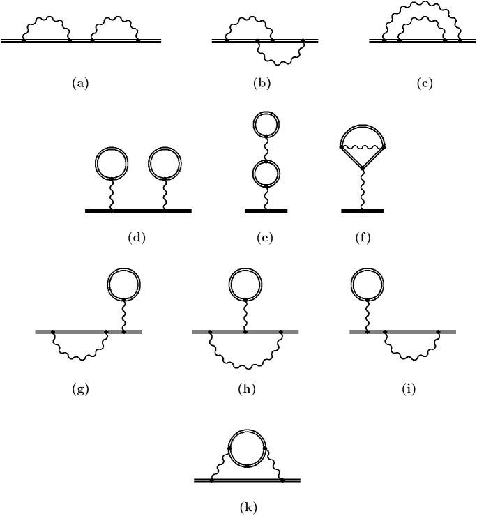
FIG. 5.: One-electron QED corrections of second order in $\alpha$.

REFERENCES

- [1] T. Stöhlker, P. H. Mokler, F. Bosch, R. W. Dunford, F. Franzke, O. Klepper, C. Kozhuharov, T. Ludziejewski, F. Nolden, H. Reich, P. Rymuza, Z. Stachura, M. Steck, P. Swiat, and A. Warczak, Phys. Rev. Lett. 85, 3109 (2000).
- [2] V. A. Yerokhin, A. N. Artemyev, V. M. Shabaev, M. M. Sysak, O. M. Zherebtsov, and G. Soff, Phys. Rev. A, in press.
- [3] K. Pachucki, Phys. Rev. A 63, 042503 (2001).
- [4] A. Mitrushenkov, L. Labzowsky, I. Lindgren, H. Persson, and S. Salomonson, Phys. Lett. A 200, 51 (1995).
- [5] S. Mallampalli and J. Sapirstein, Phys. Rev. Lett. 80, 5297 (1998).
- [6] V. A. Yerokhin, Phys. Rev. A 62 012508 (2000).
- [7] S. Mallampalli and J. Sapirstein, Phys. Rev. A 57, 1548 (1998).
- [8] I. Goidenko, L. Labzowsky, A. Nefiodov, G. Plunien, S. Zschocke, and G. Soff, In: Hydrogen atom: Precision Physics of Simple Atomic System, ed. by S. G. Karshenboim et al., (Springer, Berlin, 2001), to be published.
- [9] N. J. Snyderman, Ann. Phys. (N.Y.) 211, 43 (1991).
- [10] V. A. Yerokhin and V. M. Shabaev, Phys. Rev. A 60, 800 (1999).
- [11] J. A. Fox and D. R. Yennie, Ann. Phys. (N.Y.) 81, 438 (1973).
- [12] W. R. Johnson, S. A. Blundell, and J. Sapirstein, Phys. Rev. A 37, 307 (1988).
- [13] C. de Boor, A Practical Guide to Splines. (Springer, NY, 1978).
- [14] P. J. Mohr, G. Plunien, and G. Soff, Phys. Rep. 293, 227 (1998).
- [15] V. A. Yerokhin, A. N. Artemyev, T. Beier, G. Plunien, V. M. Shabaev, and G. Soff, Phys. Rev. A 60, 3522 (1999).
- [16] H. Persson, S. Salomonson, and P. Sunnergren, Adv. Quant. Chem. 30, 379 (1998).
- [17] V. A. Yerokhin, In: Hydrogen atom: Precision Physics of Simple Atomic System, ed. by S. G. Karshenboim et al., (Springer, Berlin, 2001), to be published.
- [18] J. D. Zumbro, E. B. Shera, Y. Tanaka, C. E. Bemis, Jr., R. A. Naumann, M. V. Hoehn, W. Reuter, R. M. Steffen, Phys. Rev. Lett. 53, 1888 (1984).
- [19] P. J. Mohr and B. N. Taylor, Rev. Mod. Phys. 72, 351 (2000).
- [20] P. J. Mohr and G. Soff, Phys. Rev. Lett. 70, 158 (1993).
- [21] G. Soff and P. Mohr, Phys. Rev. A 38 (1988) 5066.
- [22] H. Persson, I. Lindgren, L. Labzowsky, G. Plunien, T. Beier, and G. Soff, Phys. Rev. A 54, 2805 (1996).
- [23] T. Beier, G. Plunien, M. Greiner, and G. Soff, J. Phys. B 30, 2761 (1997).
- [24] T. Beier and G. Soff, Z. Phys. D 8, 129 (1988).
- [25] S. M. Schneider, W. Greiner, and G. Soff, J. Phys. B 26, L529 (1993).
- [26] G. Plunien, T. Beier, G. Soff, and H. Persson, Eur. Phys. J. D 1, 177 (1998).
- [27] S. Mallampalli and J. Sapirstein, Phys. Rev. A 54, 2714 (1996).
- [28] V. M. Shabaev, A. N. Artemyev, T. Beier, G. Plunien, V. A. Yerokhin, and G. Soff, Phys. Rev. A, 57, 4235 (1998).
- [29] G. Plunien and G. Soff, Phys. Rev. A 51, 1119 (1995); 53, 4614 (1996).
- [30] A. V. Nefiodov, L. N. Labzowsky, G. Plunien and G. Soff, Phys. Lett. A 222, 227 (1996).
- [31] N. Yamanaka, A. Haga, Y. Horikawa, and A. Ichimura, Phys. Rev. A 63, 062502 (2001).
- [32] H. Persson, I. Lindgren, S. Salomonson, and P. Sunnergren, Phys. Rev A 48, 2772 (1993).
- [33] I. Lindgren, H. Persson, S. Salomonson, V. Karasiev, L. Labzowsky, A. Mitrushenkov, and M. Tokman, J. Phys. B 26, L503 (1993).
- [34] J. Schweppe, A. Belkacem, L. Blumenfeld, N. Claytor, B. Feinberg, H. Gould, V. E. Kostroun, L. Levy, S. Misawa, J. R. Mowat, and M. H. Prior, Phys. Rev. Lett. 66, 1434 (1991).