INTRABEAM SCATTERING ANALYSIS OF ATF BEAM MEASUREMENTS

Abstract

At the Accelerator Test Facility (ATF) at KEK intrabeam scattering (IBS) is a strong effect for an electron machine. It is an effect that couples all dimensions of the beam, and in April 2000, over a short period of time, all dimensions were measured as functions of current. In this report we derive a simple relation for the growth rates of emittances due to IBS. We apply the theories of Bjorken-Mtingwa, Piwinski, and a formula due to Raubenheimer to the ATF parameters, and find that the results all agree (if in Piwinski’s formalism we replace $\eta^{2}/\beta$ by ${\cal H}$). Finally, we compare theory, including the effect of potential well bunch lengthening, with the April 2000 measurements, and find reasonably good agreement in the energy spread and horizontal emittance dependence on current. The vertical emittance measurement, however, implies that either: there is error in the measurement (equivalent to an introduction of 0.6% $x$-$y$ coupling error), or the effect of intrabeam scattering is stronger than predicted (35% stronger in growth rates).

1 INTRODUCTION

In future e+e- linear colliders, such as the JLC/NLC, damping rings are needed to generate beams of intense bunches with very low emittances. The Accelerator Test Facility (ATF)[1] at KEK is a prototype for such damping rings. In April 2000 the single bunch energy spread, bunch length, and horizontal and vertical emittances of the beam in the ATF were all measured as functions of current[2],[3]. One surprising outcome was that, at the design current, the vertical emittance appeared to have grown by a factor of 3 over the zero-current result. A question with important implications for the JLC/NLC is: Is this growth real, or is it measurement error? And if real, is it consistent with expected physical effects, in particular, with the theory of intrabeam scattering (IBS).

IBS is an important research topic for many present and future low-emittance storage rings, and the ATF is an ideal machine for studying this topic. In the ATF as it is now, running below design energy and with the wigglers turned off, IBS is relatively strong for an electron machine. It is an effect that couples all dimensions of the beam, and at the ATF all beam dimensions can be measured. A unique feature of the ATF is that the beam energy spread, an especially important parameter in IBS theory, can be measured to an accuracy of a few percent. The bunch length measurement is important since at the ATF potential well bunch lengthening is significant[3]. Evidence that we are truly seeing IBS at the ATF include (see also Ref. [4]): (1) when moving onto the coupling resonance, the normally large energy spread growth with current becomes negligibly small; (2) if we decrease the vertical emittance using dispersion correction, the energy spread increases.

Calculations of IBS tend to use the equations of Piwinski[5] (P) or of Bjorken and Mtingwa[6] (B-M). Both approaches solve the local, two-particle Coulomb scattering problem under certain assumptions, but the results appear to be different. The B-M result is thought to be the more accurate of the two, with the difference to the P result noticeable when applied to very low emittance storage rings[7]. Another, simpler formulation is due to Raubenheimer (R)[8]. Also found in the literature is a more complicated result that allows for $x$-$y$ coupling[9], and a recent formulation that includes effects of the impedance[10]. An optics computer program that solves IBS, using the B-M equations, is SAD[11].

Calculations of IBS tend to be applied to proton or heavy ion storage rings, where effects of IBS are normally more pronounced. Examples of comparisons of IBS theory with measurement can be found for proton[12],[13] and electron machines[14],[15]. In such reports, although good agreement is often found, the comparison/agreement is usually not complete (e.g. in Ref. [12] growth rates agree reasonably well in the longitudinal and horizontal, but completely disagree in the vertical) and/or a fitting or “fudge” factor is needed to get agreement (e.g. Ref. [15]).

In the present report we briefly describe IBS calculations, and derive a theorem concerning the relative vertical to horizontal IBS emittance growths in electron machines. We then compare the results of the P, B-M, and R methods, when applied to the ATF parameters. Finally, we compare the IBS growth in all beam dimensions, including the effect of potential well bunch lengthening, for the B-M calculation and the ATF data of April 2000.

Note that this is a revised version of the original report. After correcting for a $\sqrt{2}$ typo found in B-M, and after more carefully considering the Coulomb log factor, the agreement between measurement and theory has improved.

2 IBS CALCULATIONS

We begin by sketching the general method of calculating the effect of IBS in a storage ring (see, e.g. Ref. [5]). Let us first assume that there is no $x$-$y$ coupling.

Let us consider the IBS growth rates in energy $p$, in the horizontal $x$, and in the vertical $y$ to be defined as

$${1\over T_{p}}={1\over\sigma_{p}}{d\sigma_{p}\over dt}\ ,\quad{1\over T_{x}}={1\over\epsilon_{x}^{1/2}}{d\epsilon_{x}^{1/2}\over dt}\ ,\quad{1\over T_{y}}={1\over\epsilon_{y}^{1/2}}{d\epsilon_{y}^{1/2}\over dt}\ .$$ (1)

Here $\sigma_{p}$ is the rms (relative) energy spread, $\epsilon_{x}$ the horizontal emittance, and $\epsilon_{y}$ the vertical emittance. In general, the growth rates are given in both P and B-M theories in the form (for details, see Refs. [5],[6]):

$${1\over T_{i}}=\left<f_{i}\right>$$ (2)

where subscript $i$ stands for $p$, $x$, or $y$. The functions $f_{i}$ are integrals that depend on beam parameters, such as energy and phase space density, and lattice properties, including dispersion ($y$ dispersion, though not originally in B-M, can be added in the same manner as $x$ dispersion); the brackets $\langle\rangle$ mean that the quantity is averaged over the ring.

From the $1/T_{i}$ we obtain the steady-state properties for machines with radiation damping:

$$\epsilon_{x}={\epsilon_{x0}\over 1-\tau_{x}/T_{x}}\ ,\ \epsilon_{y}={\epsilon_{y0}\over 1-\tau_{y}/T_{y}}\ ,\ \sigma^{2}_{p}={\sigma^{2}_{p0}\over 1-\tau_{p}/T_{p}}\ ,$$ (3)

where subscript 0 represents the beam property due to synchrotron radiation alone, i.e. in the absence of IBS, and the $\tau_{i}$ are synchrotron radiation damping times. These are 3 coupled equations since all 3 IBS rise times depend on $\epsilon_{x}$, $\epsilon_{y}$, and $\sigma_{p}$. Note that a 4th equation, the relation between bunch length $\sigma_{s}$ and $\sigma_{p}$, is also implied; generally this is taken to be the nominal (zero current) relation.

The best way to solve Eqs. 3 is to convert them into 3 coupled differential equations, such as is done in e.g. Ref. [15], and solve for the asymptotic values. For example, the equation for $\epsilon_{y}$ becomes

$${d\epsilon_{y}\over dt}=-{(\epsilon_{y}-\epsilon_{y0})\over\tau_{y}}+{\epsilon_{y}\over T_{y}}\quad,$$ (4)

and there are corresponding equations for $\epsilon_{x}$ and $\sigma_{p}^{2}$.

Note that:

• For weak coupling, we add the term $-\kappa\epsilon_{x}$, with $\kappa$ the coupling factor, into the parenthesis of the $\epsilon_{y}$ differential equation, Eq. 4.

• A conspicuous difference between the P and B-M results is their dependence on dispersion $\eta$: for P the $f_{i}$ depend on it only through $\eta^{2}$; for B-M, through $[\eta^{\prime}+\beta^{\prime}\eta/(2\beta)]$ and the dispersion invariant ${\cal H}=\bar{\gamma}\eta^{2}+2\alpha\eta\eta^{\prime}+\beta{\eta^{\prime}}^{2}$, with $\alpha$, $\beta$, $\bar{\gamma}$ Twiss parameters.

• At the ATF, at the highest single bunch currents, there is significant potential well bunch lengthening, though we are still below the threshold to the microwave instability[3]. We can approximate the bunch lengthening effect in our IBS calculations by adding a multiplicative factor $f_{pw}(I)$ [$I$ is current], obtained from measurements, to the equation relating $\sigma_{s}$ to $\sigma_{p}$.

• The results include a so-called Coulomb log factor, of the form $\ln(b_{max}/b_{min})$, where $b_{max}$, $b_{min}$ are the maximum, minimum impact parameters, quantities which are not well defined; typically $\ln()\sim 20$. For typical, flat beams we take $b_{max}$ to be the vertical beam size, $\sigma_{y}$; $b_{min}=r_{0}c^{2}/\langle v_{x}^{2}\rangle=r_{0}\beta_{x}/(\gamma^{2}\epsilon_{x})$, with $r_{0}$ the classical electron radius ($2.82\times 10^{-15}$ m), $c$ the speed of light, $v_{x}$ the transverse velocity in the rest frame, and $\gamma$ the energy factor. For the ATF, $\ln()=16.0$.

• The IBS bunch distributions are not Gaussian, and tail particles can be overemphasized in these solutions. We are interested in core sizes, which we estimate by eliminating interactions with collision rates less than the synchrotron radiation damping rate[17]. We can approximate this in the Coulomb log term by letting $\pi b_{min}^{2}\langle|v_{x}|\rangle\langle n\rangle=1/\tau$, with $n$ the particle density in the rest frame[16]; or $b_{min}=\sqrt{4\pi\sigma_{x}\sigma_{y}\sigma_{z}/[Nc\tau]}(\beta_{x}/\epsilon_{x})^{1/4}$, with $N$ the bunch population. For the ATF with this cut, $\ln()=13.9$.

2.1 Emittance Growth

An approximation to Eqs. 2, valid for typical, flat electron beams is due to Raubenheimer (R) [8],[18]:

$${1\over T_{p}} \approx {r_{0}^{2}cN\over 32\gamma^{3}\epsilon_{x}\epsilon_{y}\sigma_{s}\sigma_{p}^{2}}\left({\epsilon_{x}\epsilon_{y}\over\langle\beta_{x}\rangle\langle\beta_{y}\rangle}\right)^{1/4}\ln\left({\langle\sigma_{y}\rangle\gamma^{2}\epsilon_{x}\over r_{0}\langle\beta_{x}\rangle}\right)$$

$${1\over T_{x,y}} \approx {\sigma_{p}^{2}\langle{\cal H}_{x,y}\rangle\over\epsilon_{x,y}}{1\over T_{p}}\quad.$$ (5)

If the vertical emittance is due only to vertical dispersion then[8]

$$\epsilon_{y0}\approx{\cal J}_{\epsilon}\langle{\cal H}_{y}\rangle\sigma_{p0}^{2}\quad,$$ (6)

with ${\cal J}_{\epsilon}$ the energy damping partition number. We can solve Eqs. 3,5,6 to obtain the steady-state beam sizes. Note that once the vertical orbit—and therefore $\langle{\cal H}_{y}\rangle$—is set, $\epsilon_{y0}$ is also determined.

Following an argument in Ref. [8] we can obtain a relation between the expected vertical and horizontal emittance growth due to IBS in the presence of random vertical dispersion: The beam momentum in the longitudinal plane is much less than in the transverse planes. Therefore, IBS will first heat the longitudinal plane; this, in turn, increases the transverse emittances through dispersion (through ${\cal H}$), like synchrotron radiation (SR) does. One difference between IBS and SR is that IBS increases the emittance everywhere, and SR only in bends. We can write

$${\epsilon_{y0}\over\epsilon_{x0}}\approx{{\cal J}_{x}\langle{\cal H}_{y}\rangle_{b}\over{\cal J}_{y}\langle{\cal H}_{x}\rangle_{b}}\quad,\quad{\epsilon_{y}-\epsilon_{y0}\over\epsilon_{x}-\epsilon_{x0}}\approx{{\cal J}_{x}\langle{\cal H}_{y}\rangle\over{\cal J}_{y}\langle{\cal H}_{x}\rangle}\ ,$$ (7)

where ${\cal J}_{x,y}$ are damping partition numbers, and $\langle\rangle_{b}$ means averaging is only done over the bends. For vertical dispersion due to errors we expect $\langle{\cal H}_{y}\rangle_{b}\approx\langle{\cal H}_{y}\rangle$. Therefore,

$$r_{\epsilon}\equiv{(\epsilon_{y}-\epsilon_{y0})/\epsilon_{y0}\over(\epsilon_{x}-\epsilon_{x0})/\epsilon_{x0}}\approx{\langle{\cal H}_{x}\rangle_{b}\over\langle{\cal H}_{x}\rangle}\quad,$$ (8)

which, for the ATF is 1.6. If, however, there is only $x$-$y$ coupling, $r_{\epsilon}=1$; if there is both vertical dispersion and coupling, $r_{\epsilon}$ will be between $\langle{\cal H}_{x}\rangle_{b}/\langle{\cal H}_{x}\rangle$ and 1.

2.2 Numerical Comparison

Let us compare the results of the P, B-M, and R methods when applied to the ATF beam parameters and lattice, with vertical dispersion and no $x$-$y$ coupling. We take: current $I=3.1$ mA, energy $E=1.28$ GeV, $\sigma_{p0}=5.44\times 10^{-4}$, $\sigma_{s0}=5.06$ mm (for an rf voltage of 300 kV), $\epsilon_{x0}=1.05$ nm, $\tau_{p}=20.9$ ms, $\tau_{x}=18.2$ ms, and $\tau_{y}=29.2$ ms; $f_{pw}=1$. The ATF circumference is 138 m, ${\cal J}_{\epsilon}=1.4$, $\langle\beta_{x}\rangle=3.9$ m, $\langle\beta_{y}\rangle=4.5$ m, $\langle\eta_{x}\rangle=5.2$ cm and $\langle{\cal H}_{x}\rangle=2.9$ mm. To generate vertical dispersion we randomly offset magnets by 15 $\mu$m, and then calculate the closed orbit using SAD. For our seed we find that the rms dispersion $(\eta_{y})_{rms}=7.4$ mm, $\langle{\cal H}_{y}\rangle=17$ $\mu$m, and $\epsilon_{y0}=6.9$ pm (in agreement with Eq. 6). For consistency between the methods we here take $\ln()=\ln{[\langle\sigma_{y}\rangle\gamma^{2}\epsilon_{x}/(r_{0}\langle\beta_{x}\rangle)]}=16$.

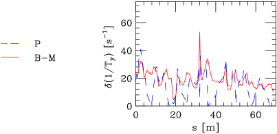
Figure 1: Vertical differential growth rate over 1/2 the ATF, for Piwinski (dashes) and Bjorken-Mtingwa (solid).

Performing the calculations, we find that the growth rates in $p$ and $x$ agree well between the two methods; the vertical rate, however, does not. Fig. 1 displays the vertical differential IBS growth rate $\delta(1/T_{y})$, over half the ring (the periodicity is 2), as obtained by the two methods (dashes for P, solid for B-M). The IBS growth rate $1/T_{y}$ is the average value of this function. We see that the P curve is enveloped by the B-M curve; the average P result is 25% less than that of B-M.

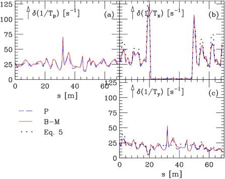
Figure 2: Differential growth rates over 1/2 the ATF, as obtained by modified Piwinski (dashes) and Bjorken-Mtingwa (solid).

From the arguments of Sec. 2.1, we might expect that we can improve the P calculation if we replace $\eta_{x,y}^{2}/\beta_{x,y}$ in the formulation by ${\cal H}_{x,y}$. Doing this we find that, indeed, the three differential growth rates now agree reasonably well with the B-M results (see Fig. 2). As for the averages, the P results are all systematically low, by 6%. According to the B-M method $1/T_{p}=27.0$ s^-1, $1/T_{x}=26.0$ s^-1, $1/T_{y}=19.4$ s^-1; $\sigma_{p}/\sigma_{p0}=1.52$, $\epsilon_{x}/\epsilon_{x0}=1.90$, $\epsilon_{y}/\epsilon_{y0}=2.30$. The emittance ratio of Eq. 8 is $r_{\epsilon}=1.44$, close to the expected 1.6.

The dots in Fig. 2b,c give the differential rates corresponding to Eq. 5, and we see that the agreement also is good. The growth rates in ($p$,$x$,$y$) are (27.0,26.4,19.3) s^-1, the relative growths in ($\sigma_{p}$,$\epsilon_{x}$,$\epsilon_{y}$) are (1.51,1.92,2.29).

3 COMPARISON WITH MEASUREMENT

The parameters $\sigma_{p}$, $\sigma_{s}$, $\epsilon_{x}$, and $\epsilon_{y}$ were measured in the ATF as functions of current over a short period of time at rf voltage $V_{c}=300$ kV. Energy spread was measured on a screen at a dispersive region in the extraction line (Fig. 3a); bunch length with a streak camera in the ring (Fig. 3b). The curves in the plots are fits that give the expected zero current result. Emittances were measured on wire monitors in the extraction line (the symbols in Fig. 4b-c; note that the symbols in Fig. 4a reproduce the fits to the data of Fig. 3). Unfortunately, we do not have error bars for this data. In $x$, nevertheless, we expect the errors to be small. In $y$, from experience, we expect the random component of errors to be 5–10%. As for the systematic component, it is conceivable that it is not small, since $\epsilon_{y}$ is small and it only takes a small amount of roll or dispersion in the extraction line to significantly affect the measurement result.

We see that $\epsilon_{x}$ appears to grow by $\sim 85\%$ by $I=3$ mA; $\epsilon_{y}$ begins at about 1.0-1.2% of $\epsilon_{x0}$, and then grows to about 3% of $\epsilon_{x0}$, implying that $r_{\epsilon}=1.8$–2.4. If we are vertical dispersion dominated, with $(\eta_{y})_{rms}=10$ mm and $\epsilon_{y0}\approx.012\epsilon_{x0}$, then the data nearly satisfies Eq. 8, $r_{\epsilon}\approx 1.6$. However, normally, after dispersion correction, the residual dispersion at the ATF is kept to $(\eta_{y})_{rms}=3$–5 mm. On the other hand, if we are coupling dominated we see that $r_{\epsilon}\approx 1$ is not well satisfied by the data.

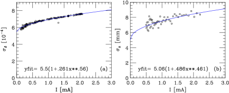
Figure 3: Measurements of energy spread (a) and bunch length (b), with $V_{c}=300$ kV.

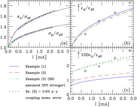
Figure 4: ATF measurement data (symbols) and IBS theory fits (the curves). The symbols in (a) give the smooth curve fits to the measured data of Fig. 3.

Let us compare B-M calculations with the data. Here we take $f_{pw}$ as given by the measurements, and take $\ln()=14$. At $I=3$ mA we adjust $\epsilon_{y0}$ until the calculated $\sigma_{p}$ agrees with the measurement. In Fig. 4 we give examples: (1) with vertical dispersion only, with $(\eta_{y})_{rms}=7.0$ mm and $\epsilon_{y0}=6.3$ pm (solid); (2) coupling dominated with $(\eta_{y})_{rms}=3$ mm and $\epsilon_{y0}=8.7$ pm (dashes); (3) increasing the strength of IBS by increasing $\ln()$ by 35%: i.e. letting $\ln()=19$, for the coupling dominated example with $(\eta_{y})_{rms}=3$ mm and $\epsilon_{y0}=14.7$ pm (dotdash); (4) same as Ex. 2 but assuming a small amount of $\epsilon_{y}$ measurement error, i.e. adding 0.6% $x$-$y$ coupling error (the dots).

We see that, for all examples, $\sigma_{p}(I)$ agrees well with measurement, and $\epsilon_{x}(I)$ agrees reasonably well also. For general agreement for $\epsilon_{y}(I)$, we need either a small amount of measurement error (e.g. 0.6% $x$-$y$ coupling measurement error), or for IBS to be 35% stronger than expected. A difference in $\ln()$ of 5 units implies a factor of 150 in the argument. Although there is uncertainty in the Coulomb log factor, this difference seems larger than we expect the uncertainty to be. Note that the expected error in the IBS calculation itself, assuming $\ln()$ is correct, is also small: $\sim 1/\ln()=5\%$[10]. And finally, note that even if we can account for the offset by e.g. a 0.6% $x$-$y$ coupling measurement error, we see from Fig. 4 that the slope of the vertical emittance dependence on current is still steeper than predicted.

4 CONCLUSION

We have derived a simple relation for relative growth rates of emittances due to IBS. We have found that for the ATF, IBS calculations following Piwinski (with $\eta^{2}/\beta$ replaced by ${\cal H}$), Bjorken-Mtingwa, and a formula due to Raubenheimer all agree well (though one needs to be consistent in choice of Coulomb log factor).

Comparing the Bjorken-Mtingwa calculations (including the effect of potential well bunch lengthening) with the ATF measurements of April 2000, we have found reasonably good agreement in the energy spread and horizontal emittance dependence on current. The vertical emittance measurement, however, implies that either: there is error in the measurement (equivalent to an introduction of 0.6% $x$-$y$ coupling error), or the effect of intrabeam scattering is stronger than predicted (35% stronger in growth rates). In addition, the slope of the vertical emittance dependence on current is steeper than predicted.

We thank A. Piwinski for help in understanding IBS and K. Oide for explaining IBS calculations in SAD.

References

- [1] F. Hinode, editor, KEK Internal Report 95-4 (1995).
- [2] J. Urakawa, Proc. EPAC2000, Vienna (2000) p. 63.
- [3] K. Bane, et al, “Impedance Analysis of Bunch Length Measurements at the ATF Damping Ring,” presented at ISEM2001, Tokyo, May 2001; SLAC-PUB-8846, May 2001.
- [4] K. Kubo, “Recent Progress in the Accelerator Test Facility at KEK,” presented at HEACC2001, Tsukuba, March 2001.
- [5] A. Piwinski, in A. Chao and M. Tigner, eds., Handbook of Accelerator Physics and Engineering (World Scientific, 1999) p. 125.
- [6] J. Bjorken, S. Mtingwa, Particle Accel. 13 (1983) 115.
- [7] A. Piwinski, private communication.
- [8] T. Raubenheimer, PhD Thesis, SLAC-387, Sec. 2.3.1, 1991.
- [9] A. Piwinski, CERN Accelerator School (1991) p. 226.
- [10] Marco Venturini, “Intrabeam Scattering and Wake Field Forces in Low Emittance Electron Rings,” this conference.
- [11] K. Oide, SAD User’s Guide.
- [12] M. Conte, M. Martini, Particle Accelerators 17 (1985) 1.
- [13] L.R. Evans and J. Gareyte, PAC85, IEEE Trans. in Nuclear Sci. NS-32 No. 5 (1985) 2234.
- [14] C.H. Kim, Proc. PAC97, Vancouver (1997) p. 790.
- [15] C.H. Kim, LBL-42305, September 1998.
- [16] K. Oide, Proc. of SAD Workshop, KEK (1998) p. 125.
- [17] T. Raubenheimer, Particle Accelerators 45 (1994) 111.
- [18] A. Piwinski, Proc. SSC Workshop, Ann Arbor (1983) p. 59.