[

Multiple beam interference in a quadrupolar glass fiber

Abstract

Motivated by the recent observation of periodic filter characteristics of an oval-shaped micro-cavity, we study the possible interference of multiple beams in the far field of a laser-illuminated quadrupolar glass fiber. From numerical ray-tracing simulations of the experimental situation we obtain the interference-relevant length-difference spectrum and compare it with data extracted from the experimental filter results. Our analysis reveals that different polygonal cavity modes being refractively output-coupled in the high-curvature region of the fiber contribute to the observed far-field interference.

]

Introduction. Optical fibers and cavities have attracted a lot of interest in recent years. On the theoretical side, a plethora of phenomena related to the interplay of classical and quantum chaos is found [2, 3]. On the experimental side, fibers are used either as (active) lasing fibers in microlasers, or as (passive) optical filters which are of great technological interest for planar integrated filter applications. Planar dielectric ring and disc cavities have been used as micron-sized optical filters mainly with evanescent light coupling, working with nearly total internal reflection. However, evanescent coupling between the cavity curved sidewall and the waveguide flat sidewall requires a very precise fabrication with a gap spacing in the sub-$\mu m$ range. Therefore, filter techniques using non-evanescent coupling which allows gap sizes larger than sub-$\mu m$ are technologically desirable.

Interestingly, recent experiments [4] using an oval-shaped micro-cavity have shown periodic output filter characteristics which are potentially useful in the above context. The purpose of this paper is to present an analysis of the experimental data and numerical ray-tracing simulations which allow a theoretical understanding of these experimental findings. Our results display a periodic filter spectrum in the far-field interference of refractively output-coupled modes of the cavity, in agreement with the experiment. We will show that the interference of multiple beam parts corresponding to polygonal round-trip orbits can lead to the observed periodic filter characteristics in a narrow window of the far-field angle.

First we briefly summarize the experiment of Ref. [4]: A passive (non-lasing) quadrupolar fiber of high-refraction glass ($n=1.8$) is illuminated by a laser beam, Fig. 1a. The tunable laser source with wavelengths in the 670 $nm$ range produces a Gaussian beam with a width (spot size) of 30 $\mu m$, the cavity axes are 150 and 180 $\mu m$. The far-field elastic scattering spectrum is measured with a linear array detector. It shows filter resonances as function of incoming wavelength with a good peak to background ratio of about 40, Fig. 2a, but only under very specific input and output coupling angles $\theta_{i,o}$ (“magic window”). The periodicity of the spectrum is a clear sign of the interference nature of the phenomenon; in addition the filter peaks display inhomogeneous broadening which is an indication of multimode interference. The light wavelength $\lambda$ is much smaller than the size of the cavity, therefore quantum effects can be assumed to be small.

FIG. 1.: a) Schematic experimental setup [4] for the filter experiment. Shown is the cross section of the oval-shaped fiber. If the input is coming from a broadband source, then the output shows periodic filter characteristics, see also Fig. 2. $\theta_{i,o}$ are the input and output angles. b) Typical orbits contributing to the far-field response, see text.

Analysis of experimental data. If we accept that the periodic output characteristics can be interpreted as interference of (classical) rays, then a length analysis of the contributing geometric paths appears suitable. We start by defining the amplitude-weighted length distribution $T(L)$ for the inferfering rays,

$$T(L)=\sum_{{\rm paths}\,i}A_{i}\,\delta(L-L_{i})\,,$$ (1)

where $A_{i}$ and $L_{i}$ are amplitude (at the detector) and optical length (from source to detector) of each path $i$ hitting the detector. The interference pattern $J(k)$ as function of the vacuum wavevector $k=2\pi/\lambda$ is given by

$$J(k) = \left|\int_{-\infty}^{\infty}{\rm d}L\,T(L)\,e^{ikL}\right|^{2}=:\int{\rm d}l\,e^{-ikl}\,S(l)\>.$$ (2)

In the last step we have introduced the length-difference spectrum $S(l)$, given by the self-convolution (correlation function) of $T(L)$, $S(l)=\int{\rm d}L\,T(L)\,T(l+L)$; for discrete paths with lengths $L_{i}$ the quantity $S(l)$ will be non-zero for $l=L_{i}-L_{j}$ $\forall\,i,j$. The length-difference spectrum $S(l)$ will be the main quantity of our analysis, it is related by Fourier transformation to the observed interference pattern $J(k)$; the information about absolute path lengths does of course not enter the interference result.

The Fourier transform $S(l)$ of a representative set of experimental data from Ref. [4] is shown in Fig. 2. We see large contributions to $S(l)$ at roughly equally spaced $l$ values, it is tempting to identify the spacing with the path length of one round trip corresponding to a single dominating cavity orbit. However, the intensity for larger $l$ is rather small, and the broad peaks suggest that more than one orbit contributes to $S(l)$. Similar results are obtained with other data sets of the experiment [4].

At this point it is useful to discuss possible interference scenarios. The simplest possibility is interference of rays tunneling out of a single stable orbit that is traced over and over again. In this case $T(L)$ contains equally spaced peaks with monotonically decreasing intensity ($\sim t(1-t)^{i-1}$ where $t$ is the tunneling rate and $i$ the number of round trips); a similar decay is then also found in the peaks of the difference spectrum $S(l)$. For the particular case of the quadrupolar fiber a candidate stable orbit is the “diamond”, here the tunneling rate is rather small. From this one would expect a slow, monotonous decay of the peak intensities in $S(l)$ – obviously this is not in agreement with the experimental data. Furthermore, in the present experimental geometry the diamond-like orbit cannot be excited by refractive input coupling, but only by tunneling – the resulting intensity is much lower than for refractive coupling, and is too small to account for the experimental observation. Other orbits like rectangular/trapezoidal modes or whispering-gallery (WG) orbits [3] are either unstable or cannot be excited with the present non-evanescent coupling. We are therefore lead to consider the interference of rays from multiple orbits as explanation for the observations of Ref. [4].

FIG. 2.: Representative experimental spectrum of Ref. [4]. a) raw interference data, $J(k)$, plotted as function of the wavevector $k$, $\theta_{i}=60^{\rm o}$, $\theta_{o}=56^{\rm o}$. b) Modulus [7] of the Fourier transform of $J(k)$ corresponding to the length-difference spectrum $S(l)$. The strong decay of the peak intensity for lengths $l$ longer than 3 or 4 round trips is a characteristic feature.

Ray-tracing simulations. We focus a two-dimensional geometry representing the cross-section of the fiber used in the experiment, see Fig. 1a. The geometry is defined by the mean radius $R$ of the cavity ($R=82\,\mu m$ in Ref. [4]) and its excentricity $\epsilon\approx 0.1$. The quadrupole boundary is given by $r(\phi)=R(1\!+\!\epsilon\cos 2\phi)$ in polar coordinates, and the lengths of the half axes are $R(1\pm\epsilon)$.

The incoming beam is discretized into a sufficiently high number of equally spaced parallel rays, for simplicity we employ a rectangular beam profile. The intensity fraction of each ray that penetrates into the quadrupole is given by the Fresnel formula, its angle by Snell’s law. Quantum effects are negligible due to $\lambda\ll R$. The dynamics of each ray is then governed by the laws of a “Fresnel billiard” [3, 5], i.e., by straight propagation, specular reflection at the quadrupolar shaped boundaries, and evolution of the intensity according to Fresnel’s law for reflection and transmission. In particular, for TE polarisation [4] the Fresnel laws for the reflected (transmitted) electric field strength $E_{r}$ ($E_{t}$) for a incoming field $E_{i}$ are given by [6]

$$q_{r}:=\frac{E_{r}}{E_{i}} = \frac{\cos\chi-n\sqrt{1-n^{2}\sin^{2}\chi}}{\cos\chi+n\sqrt{1-n^{2}\sin^{2}\chi}}\>,$$ (3)

$$q_{t}:=\frac{E_{t}}{E_{i}} = \sqrt{1-q_{r}^{2}}\,,$$ (4)

where $n$ is the refractive index of the cavity material, $n=1$ outside the cavity, and $\chi$ is the boundary angle of incidence, Fig. 1. Strictly, these relations hold for a planar interface; modified Fresnel formulae for curved interfaces can be derived [9], but in the present case of a very large size parameter, $R\gg\lambda$, the curvature effect is negligible. We assume perfectly reflecting walls for angles of incidence $\chi$ bigger than the critical angle, $\chi_{c}=\arcsin(1/n)$, and exclude leakage due to quantum tunneling.

In the simulation, we trace each ray of the incoming beam numerically to construct the interference pattern [3, 8]. For angles $\chi<\chi_{c}$ we allow for refractive escape of the part of the ray that is determined by Eq. (4), but follow further the remaining part inside the quadrupole until its intensity falls below a threshold of $10^{-6}$ of the initial intensity due to subsequent subcritical reflections. For the transmitted part, we determine the far field angle of the leaving ray again by Snell’s law.

In Fig. 1b we show a couple of typical trajectories that are found upon scanning of the incoming beam. Due to the finite excentricity and the finite beam width we find not only WG orbits but a large number of orbits which escape (as well as enter) around the points of highest curvature of the quadrupole, as known from the study of asymmetric resonance cavities [3, 8]. In particular, we find rays that undergo several polygonal-like round trips (in contrast to typical WG orbits they come closer to the center of the quadrupole) before their intensity eventually drops below the threshold. This process of intensity loss may happen at one single reflection or (more likely) upon a couple of subsequent reflections/transmissions. Due to the preferred escape points near the highest wall curvature [3], the distribution of the orbit lengths, measured from entering the fiber until escape, is sharply peaked at integer multiples of half the length of a round trip. Orbits with approximately 0.5, 1.5, 2.5 round trips are shown in Fig. 1b – these (and similar longer) orbits contribute to the far-field interference for an output angle as chosen in Fig. 1a, i.e., for output points opposite to the incident beam.

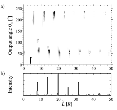
FIG. 3.: Results of the ray-tracing simulation. a) Intensity histogram showing the distribution of orbit lengths $\widetilde{L}$ vs their output angle $\theta_{o}$. The gray scale indicates the intensity (black - maximal). The input angle is fixed at $\theta_{i}=60^{o}$. b) Intensity vs. orbit length $\widetilde{L}$ at a specific detector position (in the “magic window”, see text), obtained by integrating the above histogram over a narrow interval of output angles, $58^{o}<\theta_{o}<62^{o}$. If we neglect external path differences this quantity is equivalent to the length distribution $T(L)$.

Given the experimental findings, we are especially interested in rays with escape direction within the “magic window”. The filter characteristics was observed in the far-field total intensity – in this situation the detector is placed at a distance large compared to the cavity radius. Therefore only rays within a narrow window of the output angle $\theta_{o}$ are detected, whereas the exact escape position on the quadrupolar boundary is of no importance. In contrast, in a near field measurement (usually done with a focussing lens) a narrow interval of output positions is sampled, with a rather large range of output angles.

We now turn to the ray-tracing simulation results for the far-field interference. The primary output of the simulation are the ray trajectories, their escape points and output angles, and the output (transmission) intensities which result from the Fresnel formulae (4). Fig. 3a shows lengths $\widetilde{L}$ and output angles $\theta_{o}$ in the form of a intensity histogram plot (“Fresnel-weighted” histogram) for a fixed input angle $\theta_{i}=60^{o}$. Here, $\widetilde{L}$ are the geometric orbit lengths inside the cavity in units of $R$; the optical lengths are found from $L=n\widetilde{L}R+L_{\rm ext}+L_{\rm phase}$, where $L_{\rm ext}$ are external length differences arising from the different input and output points of the interfering rays, and $L_{\rm phase}$ is determined by the phase shifts that occur upon the reflections. Note that the quantity shown in Fig. 3a is the output-angle-resolved version of the length spectrum $T(L)$ defined in (1). For most output angles, the intensities are rather small, and arise primarily from short lengths $\widetilde{L}$. However, in a narrow window which corresponds to escape points in the high-curvature region, the total output intensity is larger, and short as well as longer orbits carry significant weight.

If we now integrate the above quantity over a small range of far-field angles corresponding to the angle range convered by the detector, we obtain the length spectrum $T(\widetilde{L})$, shown in Fig. 3b. The peaks are easily found to correspond to orbits as shown in Fig. 1b (and longer ones). After converting $\widetilde{L}$ into optical lengths $L$, we obtain from $T(L)$ the length-difference spectrum $S(l)$ by self-convolution, and by Fourier transformation [10] the resulting interference pattern $J(k)$ as function of the wavevector $k=2\pi/\lambda$, Fig. 4.

FIG. 4.: Theoretical ray-tracing result, for the parameters $\theta_{i}=60^{o}$, $\theta_{o}=60^{o}$, and $\epsilon=$ 0.1, for details see text. The axes are as in Fig. 2.

Qualitative agreement between experiment and theory is most easily checked by comparing the length-difference spectra $S(l)$, Figs. 2b and 4b. The main feature, namely a number of roughly equally spaced peaks with comparable intensity, but very little intensity at larger lengths, is nicely reproduced by the ray-tracing data.

We note that one cannot expect to reach a quantitative agreement with experiment due to the uncertainty in experimental parameters like size and excentricity of the fiber and angle of the illuminating laser beam. The precise interference pattern depends strongly on these parameters, in particular it is extremely sensitive to length changes of the order of the light wavelength. For this reason we have neglected both $L_{\rm ext}$ and $L_{\rm phase}$ when plotting Fig. 4. These contributions to the optical length are of the order of one or several wavelengths, and are certainly smaller than the uncertainty in the fiber size. We have checked that the interference pattern depends only slightly on the numerical discretization procedure used for the incoming beam.

By varying input and output angles, our simulation data clearly show that in most situations the rays from all parts of the incident beam travel in polygonal cavity orbits only for a very short time (up to 2 round trips) before they leave the cavity via refraction. Only for a narrow range of input angles an appreciable part of the beam leads to polygonal orbits with a longer lifetime, which then are refractively output-coupled after a larger number of round trips into a narrow window of far-field angles. The far-field output angle window depends sensitively on the input angle, so we predict that the “magic window” as observed in Ref. [4] will move (in the far-field angle) with varying input angle of the beam. In particular, for $\theta_{i}=70^{o}$ we found the magic window at output angles $10^{o}$ smaller than for $\theta_{i}=60^{o}$, whereas for $\theta_{i}=50^{o}$ the filter effect almost disappears.

In addition, a number of conditions have to be met to observe the cavity filter effect: (i) A finite excentricity of the fiber is needed to produce (chaotic) orbits which come close to the center of the quadrupole and leave it by refraction preferrably near the points of highest curvature. (ii) The intensity loss per round trip should be neither too small nor too large. In the former case, too many individual orbits (with slightly different lengths) contribute to the far-field interference leading to an incoherent response, whereas in the latter case the number of contributing beams is too small to produce a sharp interference pattern. This puts constraints on the refractive index of the fiber. We have performed simulations with other fiber geometries and refraction indices which confirm the points (i) and (ii) above: using e.g. $n=1.5$ the filter effect disappears.

Summary. Our ray-tracing model appears to describe the main features found in the experiment [4]. In particular, the range of input and output angles, where far-field interference with filter characteristics can be observed, is rather small (“magic window”). The analysis of the length-difference spectrum allows for a clear distinction between our model of interfering rays from different orbits and other scenarios involving a single orbit only. We note that the TE polarization used in Ref. [4] allows for a very efficient Brewster-angle input and output fiber coupling.

Issues to be discussed in future work include (i) a comparison to the case of TM polarization, (ii) the precise connection of the observed interference to chaotic cacity trajectories, and (iii) possible application of the filter effect for beam and/or cavity diagnostics.

We are grateful to A. W. Poon for providing the experimental data of Ref. [4], furthermore we acknowledge useful discussions with R. K. Chang, J. U. Nöckel, A. W. Poon, A. D. Stone, and J. P. Wolf. This work has been supported by the DAAD and the DFG.

REFERENCES

- [1]
- [2] M. C. Gutzwiller, Chaos and Quantum Physics, Springer, New York 1990.
- [3] J. U. Nöckel and A. D. Stone, Nature 385, 45 (1997).
- [4] A. W. Poon, P. A. Tick, D. A. Nolan, and R. K. Chang, Opt. Lett., in press (2001).
- [5] M. V. Berry, Eur. J. Phys. 2, 91 (1981).
- [6] N. S. Kapany, Fiber Optics: Principles and Applications, Academic Press (New York, London), 1967.
- [7] By definition, is real and symmetric, , and the same holds for , since is real. However, the numerical Fourier transform of , taken from a finite interval , can acquire a phase factor, which is removed by working with the modulus.
- [8] J. A. Lock et al., Appl. Optics 37, 1527 (1998).
- [9] A. W. Snyder and J. D. Love, IEEE Trans. MTT 23, 134 (1975); M. Hentschel and H. Schomerus, to be published.
- [10] Fourier transformations and convolutions are performed using the Fast Fourier Transform (FFT) method as described in: W. H. Press et al., Numerical Recipes in C, Cambridge University Press, 1992.