Passive scalar anisotropy in a heated turbulent wake: new observations and implications for LES

Abstract

The effects of passive scalar anisotropy on subgrid-scale (SGS) physics and modeling for Large-Eddy Simulations are studied experimentally. Measurements are performed across a moderate Reynolds number wake flow generated by a heated cylinder, using an array of four X-wire and four cold-wire probes. By varying the separation distance among probes in the array, we obtain filtered and subgrid quantities at three different filter sizes. We compute several terms that comprise the subgrid dissipation tensor of kinetic energy and scalar-variance and test for isotropic behavior, as a function of filter scale. We find that whereas the kinetic energy dissipation tensor tends towards isotropy at small scales, the SGS scalar-variance dissipation remains anisotropic independent of filter scale. The eddy-diffusion model predicts isotropic behavior, whereas the nonlinear (or tensor eddy diffusivity) model reproduces the correct trends, but overestimates the level of scalar dissipation anisotropy. These results provide some support for so-called mixed models but raise new questions about the causes of the observed anisotropy.

1 Introduction

The statistics and general structure of passive scalars in turbulent flows differ significantly from those of the turbulent velocity field. In particular, conclusive experimental (e.g. Stewart 1969, Sreenivasan, Antonia & Britz 1979, Mestayer 1982, and Mydlarski & Warhaft 1998a) and numerical (e.g. Holzer & Siggia 1994) evidence shows that structure functions and the derivative skewness of the scalar field do not follow predictions from isotropy at inertial and dissipative scales, in the presence of a mean scalar gradient. In particular, the deviations are thought to be related to “ramp and cliff structures” and to imply a direct effect of large-scale structures on small-scale structures. The data relevant to this question has been reviewed by Sreenivasan (1991) and more recently by Warhaft (2000). Moreover, scalar spectra display a distinctly less universal structure than velocity spectra. This is manifested both in terms of spectral exponents, as well as in terms of the dimensionless spectral coefficient $c_{\theta}$. The latter varies from values near 0.4 in many experiments in the atmospheric surface layer and grid turbulence (see Sreenivasan 1991, Sreenivasan 1996 and Warhaft 2000) to $c_{\theta}\sim 1.8$ for other atmospheric measurements (Antonia, Ould-Rouis, Anselmet & Zhu 1997, and Antonia, Xu & Zhou 1999). From a fundamental point of view, these observations challenge the Kolmogorov cascade phenomenology for the transfer of scalar-variance from large to small scales. In the classical phenomenology, the multiplicity of separate “eddy breakdown” events is assumed to gradually uncouple the small from the large scales, allowing the former to tend to a universal and isotropic structure more or less independent of the large scales. On the contrary, the scalar-field measurements suggest a direct linkage among largest and smallest scales.

The coupling among scales is an important ingredient in Large-Eddy Simulations (LES). In LES, the turbulent fields (velocity and scalar) are decomposed into large and small (subgrid-scale, SGS) scale contributions by means of a spatial low-pass filter of characteristic width $\Delta$. The resulting equations which can be numerically discretized with mesh-spacing of the order of $\Delta$ require closure of the unresolved momentum fluxes (SGS stress tensor, $\tau_{ij}\equiv\widetilde{u_{i}u_{j}}-\widetilde{u}_{i}\widetilde{u}_{j}$, where a tilde represents filtering at scale $\Delta$) and scalar fluxes (e.g. the SGS heat flux, $q_{j}\equiv\widetilde{\theta u_{j}}-\widetilde{\theta}\widetilde{u}_{j}$ where $\theta$ is the passive scalar field). The promise of LES is often predicated upon small-scale universality and isotropy, and the absense of a strong coupling across disparate length scales. Hence, the observed anisotropy of the scalar field seems to pose a challenge to the very foundation of LES. While these deviations from classical phenomenology are now quite well established, little is known about their impact on the closure problem for LES. The present work quantifies the implications of small-scale scalar anisotropy on quantities that describe subgrid-scale physics and directly affect modeling for LES.

As reviewed in Meneveau & Katz (2000), the most important statistical property of the fluxes $\tau_{ij}$ and $q_{j}$ is how they affect the mean kinetic energy and scalar-variance budgets of the resolved fields. Specifically, their dominant effect is through the kinetic energy and scalar-variance dissipations that arise from interactions between subgrid and resolved scales. Therefore, in the present study, we mainly focus on the so-called SGS kinetic energy dissipation $-\langle\tau_{ij}\widetilde{S}_{ij}\rangle$ (Piomelli et al. , 1991) and scalar-variance dissipation $-\langle q_{j}\widetilde{G}_{j}\rangle$ (Porté-Agel, Meneveau & Parlange 1998). Here $\widetilde{S}_{ij}\equiv\frac{1}{2}\big{(}\partial\widetilde{u}_{i}/\partial x_{j}+\partial\widetilde{u}_{j}/\partial x_{i}\big{)}$ and $\widetilde{G}_{j}\equiv\partial\widetilde{\theta}/\partial x_{j}$ are the resolved strain-rate tensor and scalar gradient, respectively. The SGS dissipation rates represent the flux (cascade) of kinetic energy or scalar-variance from resolved towards subgrid scales (when positive). When $\Delta$ pertains to the inertial range, and when the flow is in equilibrium, one expects the mean SGS dissipation to equal the molecular dissipation rate.

Deviations from isotropy in the context of SGS dissipation can be probed by measuring the isotropy level of the tensors $-\langle\tau_{ij}\widetilde{S}_{mn}\rangle$ and $-\langle q_{i}\widetilde{G}_{j}\rangle$, as a function of scale. The main question to be addressed in this work is whether the approach to isotropy (if it exists) is the same for kinetic energy and scalar-variance dissipation tensors. Another goal is to test the ability of two popular model classes (eddy diffusivity and nonlinear models, see Meneveau & Katz 2000 for a review) to reproduce the observations. In order to span a sizeable range of inertial-range filter scales, a sufficiently high Reynolds number must be considered. Hence, this study is based on experimental data (as opposed to DNS which is limited to small Reynolds numbers). The study is performed in a canonical shear flow, the heated cylinder wake.

2 Experiment apparatus and flow characteristics

Experiments were performed in the return type Corrsin Wind Tunnel (Comte-Bellot & Corrsin 1966). A heated smooth cylinder of diameter $D$ = 4.83 cm was located horizontally at the centerline of the test section. The measurement location in the streamwise direction $(x_{1})$ was fixed at $x_{1}/D=25$. To obtain the filtered and SGS quantities, an array of four custom-made miniature probes was used. Each probe was composed of one X-type hot-wire and one I-type cold-wire for the velocities in the $x_{1}-x_{2}$ plane and the temperatures, respectively. Here $x_{2}$ is the “cross-wake” direction, i.e. perpendicular to $x_{1}$ and to the cylinder axis.

The separation distance $h$ between the probes in the cross-wake direction $x_{2}$ could be adjusted manually between 5 and 20 mm. Three configurations ($\Delta=2h$, with $h=5$, 10 and 20 mm) were used in the present study. A 2.5 $\mu$m platinum-coated tungsten wire which had been copper-plated was soldered on to the X-wire prong ends and etched, yielding an active length-to-diameter ratio of about 200. The wire spacing between the hot-wires was 0.5 mm. A 0.625 $\mu$m silver-coated pure platinum wire for a cold-wire sensor was soldered on the I-wire prong ends and subsequently etched. To minimize the low frequency amplitude attenuation, the active length-to-diameter ratio was about 1000 as suggested by [Bruun (1995)]. The separation distance between the cold-wire and its nearest hot-wire was 0.9 mm so that the thermal effect from the hot-wire on the cold-wire was negligible. The signals were low-pass filtered at a frequency of 20 kHz and sampled at $f_{s}=40$ kHz. Sampling time was 60 seconds, so the total number of data points per channel for each measurement location was $2.4\times 10^{6}$. The array was traversed across the wake, and data were recorded at 17 discrete cross-wake locations from the centerline to the wake edge at increments of 14.4 mm.

At the measurement location of $x_{1}/D=25$, the mean centerline velocity $(U_{CL})$ was $13.6$ m/s, the defect velocity $(U_{d}=U_{\infty}-U_{CL})$ was $4.4$ m/s, the defect temperature $(\theta_{d}=\theta_{CL}-\theta_{\infty})$ was $0.61~{}^{\circ}$C, and the half-width of the wake was $\ell=0.08$ m. To get the spatial quantities along the streamwise direction from the temporal data, Taylor’s hypothesis was invoked. The turbulence intensity of the streamwise velocity at the centerline was about $13.3\%$. The molecular kinetic energy dissipation at the centerline $(\epsilon_{CL})$ was $87$ m²s^-3, and the molecular scalar-variance dissipation at the centerline $(\epsilon_{\theta CL})$ was $0.65~{}^{\circ}$C²s^-1. The latter two variables were obtained from (corrected) third-order structure functions as in Cerutti et al. (2000) and [Lindborg (1999)]. It follows that the Kolmogorov length scale $(\eta=(\nu^{3}/\epsilon)^{1/4})$ was $0.08$ mm, the Taylor micro-scale $(\lambda)$ was $2.9$ mm, and the Reynolds number based on Taylor micro-scale $(Re_{\lambda})$ was $350$. The longitudinal integral scale obtained by integrating up to the first zero crossing of the $u_{1}$ correlation function was $L_{11}=0.091$ m. Profiles of mean velocity, rms velocities, Reynolds shear stress, rms temperature and heat flux distributions across the wake agreed quite well with results in the literature (e.g., Matsumura & Antonia 1993 and Kiya & Matsumura 1988).

In the present study, to separate between large and small scales, the box filter is applied to the streamwise and cross-wake directions, and the trapezoidal rule is used for the spatial integrations. The filtering process consists in a discrete approximation to a two-dimensional box filter. In the $x_{2}$ direction, a four point discretization is used for evaluating the SGS fluxes while a three-point approximation is used for the filtered derivatives. Filtered velocity and scalar gradients in the $x_{2}$ direction are evaluated using first-order finite differences over a distance $h$. In the streamwise direction, the box filter is approximated using $\Delta f_{s}/\langle u_{1}\rangle$ sampling points and the $x_{1}$ derivatives are evaluated using finite differences over a distance $h$. The filtering and error analysis is documented in Cerutti & Meneveau (2000) and Cerutti et al. (2000).

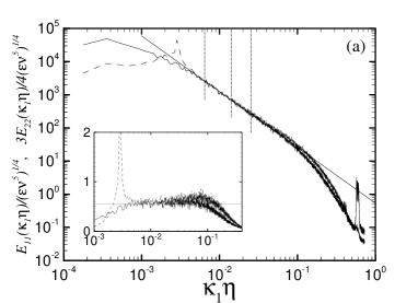
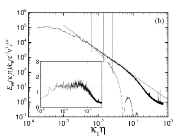
Figure 1: Velocity and temperature spectra at the centerline, in Kolmogorov units: (a) the longitudinal spectrum of the $u_{1}$ component (solid line) and the longitudinal spectrum of the $u_{2}$ component multiplied by 3/4 (dashed line), as a function of the longitudinal wavenumber, $\kappa_{1}$. The spectrum of $u_{2}$ component is below that of $u_{1}$ at low wave number ($\kappa_{1}\eta<0.002$) with a Strouhal peak ($\kappa_{1}\eta\sim 0.003$), and higher at high wave number ($0.1<\kappa_{1}\eta<0.4$); (b) the longitudinal spectrum of the temperature (solid line) and of the filtered temperature, filtered at $\Delta/\eta=125$ (dashed line). The inserts in (a) and (b) show the compensated spectra, $E_{11}(\kappa_{1})~{}\epsilon^{-2/3}\kappa_{1}^{5/3}$, $\frac{3}{4}E_{22}(\kappa_{1})~{}\epsilon^{-2/3}\kappa_{1}^{5/3}$ and $E_{\theta\theta}(\kappa_{1})~{}\epsilon_{\theta}^{-1}\epsilon^{1/3}\kappa_{1}^{5/3}$. The three vertical dotted lines in (a) and (b) are the wavenumbers corresponding to the filter sizes of $\Delta/\eta=$125 (10 mm), 250 (20 mm), 500 (40 mm). The straight solid lines are the universal spectra (see text).

Figure 1(a) shows a comparison between the longitudinal spectrum $E_{11}(\kappa_{1})$ of the $u_{1}$ component and the longitudinal spectrum $E_{22}(\kappa_{1})$ of the $u_{2}$ component multiplied by 3/4 at the centerline. Here, $\kappa_{1}$ is the longitudinal wave number. The three vertical dashed lines correspond to the filter sizes of ${\Delta/\eta=}$125 (10 mm), 250 (20 mm), 500 (40 mm). All the filter sizes are in the inertial range. Since the noise peak in the longitudinal spectrum of $u_{1}$ is in the far dissipation region, quite removed from any of the filter frequencies and scales of interest in this study, no effort is made to remove the noise by additional filtering (various attempts such as notch filtering showed no effect on the results). It can be clearly observed that $E_{11}(\kappa_{1})\approx{3\over 4}E_{22}(\kappa_{1})$ as required by isotropy in the inertial range, over about one decade of wave numbers. The peak in $E_{22}(\kappa_{1})$ at $\kappa_{1}\eta\sim 0.003$ is due to the periodic von Kármán vortex street behind the cylinder. The frequency of the vortices is 78.1 Hz, and this gives Strouhal number $S_{t}~{}(=fD/U_{\infty})=0.211$. The Kolmogorov constant $c_{K}$ in $E_{11}(\kappa_{1})=\frac{18}{55}c_{K}\epsilon^{2/3}\kappa_{1}^{-5/3}$ is obtained as $c_{K}=\frac{55}{18}(0.56)=1.71$ in the insert. This value is quite close to the standard value of 1.6 (see review by Sreenivasan 1995) and a similar value of 1.7 was observed by O’Neil & Meneveau (1997). Figure 1(b) shows the longitudinal spectrum of the temperature $E_{\theta\theta}(\kappa_{1})$. As seen in the premultiplied spectrum shown in the insert, there is a fairly clear inertial range with a $-5/3$ slope. This slope is steeper than those found in the round jet by Tong & Warhaft (1995) and Miller & Dimotakis (1996), and in several other shear flows reviewed in Sreenivasan (1996). It is closer to results quoted in Antonia & Pearson (1997), who report a scaling exponent of 0.65-0.66 for the $2^{nd}$-order temperature structure function in the heated cylinder wake at $Re_{\lambda}=230$, or to the spectra for grid turbulence of Mydlarski & Warhaft (1998b).

The coefficient $c_{\theta}$ in $E_{\theta\theta}(\kappa_{1})=c_{\theta}\epsilon_{\theta}\epsilon^{-1/3}\kappa_{1}^{-5/3}$ deduced from this spectrum is about 1.4. It is significantly higher than results quoted in Sreenivasan (1996) for high Reynolds numbers, but is within the range of results from various shear flow measurements reported in Antonia et al. 1999. As discussed in Sreenivasan (1996), the dissipation measurements are based on assuming scalar isotropy and are thus subject to considerable uncertainty. On the other hand, at the centerline we find good isotropy (see section 3) which would seem to support our current estimates of the dissipation and $c_{\theta}$. While the universality of $c_{\theta}$ and spectral exponent is not the main subject of this paper, the scatter of results certainly supports the view that the scalar spectrum for shear flows at moderate Reynolds numbers (e.g. $Re_{\lambda}<1000$) depends upon details of the generation of the flow (Sreenivasan, 1996). Specifically, it seems that the dependence of the spectral exponent and prefactor on $Re_{\lambda}$ is not universal.

The longitudinal spectrum of the filtered temperature is shown as the dashed curve in figure 1(b). The lobes at scales below the filter size are due to the streamwise box filter used in the present study. Spectra of filtered velocity (not shown) have similar shape.

3 Isotropy of real SGS dissipation and model predictions

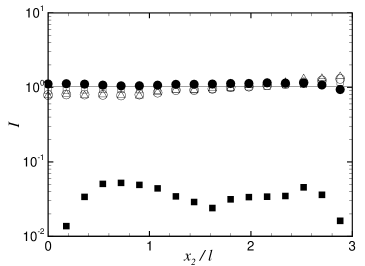
Figure 2: Isotropy ratios of the filtered gradient fields and of the mean SGS stresses across the heated wake at $x_{1}/D=25$ with the filter size of $\Delta/\eta=125$. The symbols represent: $\circ$, $\langle\widetilde{S}_{22}\widetilde{S}_{22}\rangle/\langle\widetilde{S}_{11}\widetilde{S}_{11}\rangle$; $\square$, $\langle\widetilde{S}_{12}\widetilde{S}_{12}\rangle/\langle\frac{3}{4}\widetilde{S}_{11}\widetilde{S}_{11}\rangle$; $\vartriangle$, $\langle\widetilde{G}_{2}\widetilde{G}_{2}\rangle/\langle\widetilde{G}_{1}\widetilde{G}_{1}\rangle$; $\bullet$, $\langle\tau_{22}\rangle/\langle\tau_{11}\rangle$; $\blacksquare$, $-\langle\tau_{12}\rangle/\langle\tau_{11}\rangle$.

In discussing isotropy of various tensors, we distinguish second-rank and fourth-rank tensors. Examples of second-rank tensors are the mean SGS stress $\langle\tau_{ij}\rangle$, the filtered scalar-gradient $\langle\widetilde{G}_{i}\widetilde{G}_{j}\rangle$, and the SGS scalar-variance dissipation $-\langle q_{i}\widetilde{G}_{j}\rangle$. Their isotropic form can be written as $\langle\tau_{ij}\rangle=\langle\tau_{11}\rangle\delta_{ij}$, $\langle\widetilde{G}_{i}\widetilde{G}_{j}\rangle=\langle\widetilde{G}_{1}\widetilde{G}_{1}\rangle\delta_{ij}$, and $\langle q_{i}\widetilde{G}_{j}\rangle=\langle q_{1}\widetilde{G}_{1}\rangle\delta_{ij}$ respectively. On the other hand, the strain-rate-product tensor $\langle\widetilde{S}_{ij}\widetilde{S}_{pq}\rangle$ and SGS dissipation tensor $\langle\tau_{ij}\widetilde{S}_{pq}\rangle$ are fourth-rank tensors. Their isotropic form can be written as

$$\left<\tau_{ij}\widetilde{S}_{pq}\right>=-\frac{1}{2}\left<\tau_{11}\widetilde{S}_{11}\right>\left[\delta_{ij}\delta_{pq}-\frac{3}{2}\left(\delta_{ip}\delta_{jq}+\delta_{iq}\delta_{jp}\right)\right],$$ (1)

and a similar expression holds for $\langle\widetilde{S}_{ij}\widetilde{S}_{pq}\rangle$ by replacing $\tau_{ij}$ with $\widetilde{S}_{ij}$. To derive the above expression, we have used the tensor symmetry (in $i-j$ or $p-q$) and the divergence-free condition ($\widetilde{S}_{kk}=0$). It follows that $\langle\widetilde{S}_{22}\widetilde{S}_{22}\rangle=\langle\widetilde{S}_{11}\widetilde{S}_{11}\rangle$ and $\langle\widetilde{S}_{12}\widetilde{S}_{12}\rangle=\frac{3}{4}\langle\widetilde{S}_{11}\widetilde{S}_{11}\rangle$.

Figure 2 shows isotropy ratios of the filtered gradient fields and of the mean SGS stresses, for $\Delta/\eta=125$. In isotropic conditions, all ratios have to be on the unit line except $\langle\tau_{12}\rangle/\langle\tau_{11}\rangle$ which should tend to zero with decreasing filter scale since the fraction of mean shear stress carried by the SGS scales is expected to vanish when $\Delta/\ell\to 0$. As can be seen, both the SGS stress and strain-rate fields are quite isotropic across the heated wake flow at this scale. For the larger filter sizes of $\Delta/\eta=250$ and $500$ (not shown), the trends are similar to figure 2 but slightly less isotropic.

Next, results are given for the SGS dissipation tensors across the wake. We define the following ‘isotropy ratios’:

$$I_{u22}\equiv\frac{\left<\tau_{22}\widetilde{S}_{22}\right>}{\left<\tau_{11}\widetilde{S}_{11}\right>},~{}~{}~{}I_{u12}\equiv\frac{\left<\tau_{12}\widetilde{S}_{12}\right>}{\frac{3}{4}\left<\tau_{11}\widetilde{S}_{11}\right>},~{}~{}~{}I_{\theta}\equiv\frac{\left<q_{2}\widetilde{G}_{2}\right>}{\left<q_{1}\widetilde{G}_{1}\right>}.$$ (2)

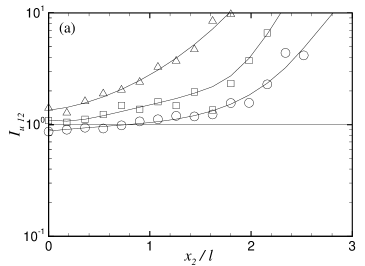
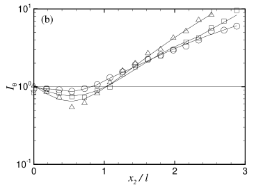
Figure 3: Isotropy ratios in the SGS dissipations: (a) $I_{u12}$; (b) $I_{\theta}$ (see Eq. 2). The symbols represent: $\circ$, $\Delta/\eta=125$; $\square$, $\Delta/\eta=250$; $\vartriangle$, $\Delta/\eta=500$. For clarity, $4^{th}$-order polynomial fits of $logI$ vs $x_{2}/\ell$ are added as solid lines.

Figures 3(a) and (b) show the spatial distributions of the SGS kinetic energy dissipation isotropy ratios $I_{u12}$ and the SGS scalar-variance dissipation isotropy ratios $I_{\theta}$, respectively, across the wake flow with the different filter sizes. All moments in this study are statistically well converged. For example, running averages such as $n^{-1}\sum_{k=1}^{n}q_{i}\tilde{G}_{j}$ did not differ from their global average by more than 6% over the last 80% of data (i.e. for $n\in[0.2N,N]$ where $N=2.4\cdot 10^{6}$). For different filter sizes considered, the SGS kinetic energy and scalar-variance dissipations are isotropic only towards the centerline of the wake. Towards the edges of the wake, large anisotropies persist (even though there the mean shear and mean temperature gradients vanish also). The isotropy ratio of $I_{u12}$ at a fixed $x_{2}/\ell$ in figure 3(a) clearly increases with the filter size. However, the isotropy ratio of the scalar-variance dissipation $I_{\theta}$ shows almost no variation with filter size for $1<x_{2}/\ell<2$, where the scalar gradient in the cross-wake direction, $\frac{\partial\theta}{\partial x_{2}}$, is large.

The increased anisotropy in the outer regions of the wake (see figures 3(a) and (b)) is another striking result. The anisotropy may be associated with the highly intermittent character of the flow there. One may wonder whether the anisotropy arises from a superposition of distinct behaviors in the turbulent and the non-turbulent (outer) regions. Using conditional averaging, O’Neil & Meneveau (1997) already showed that the conditional averages of the SGS dissipations in the non-turbulent regions were negligible compared to those in the turbulent regions. The implication was that the global averages of dissipation could be explained entirely by their conditional mean value inside the turbulent part: $\langle\tau_{ij}\tilde{S}_{ij}\rangle\approx\Gamma\langle\tau_{ij}\tilde{S}_{ij}\rangle_{T}$, where $\Gamma(x_{2})$ is the intermittency function (i.e. the fraction of time the signal is turbulent at any given $x_{2}$), and the subscript “$T$” stands for averaging conditioned on ‘turbulence’ (see O’Neil & Meneveau 1997 for details). When replacing the conditional averages multiplied by $\Gamma$ in the expression for isotropy ratios, $\Gamma$ cancels from both numerator and denominator. This behavior suggests that the anisotropy ratios shown in figure 3 are equal to those inside the turbulent regions alone, and that their rise in the outer parts of the wake cannot be explained by contributions coming from the non-turbulent parts. However, it is still possible that non-trivial contributions to the scalar-variance dissipations could originate at the interface separating turbulent from non-turbulent regions.

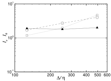
Figure 4: Isotropy ratios of kinetic energy and scalar-variance SGS dissipations at $x_{2}/\ell=1.44$, where the mean temperature gradient peaks. The open symbols (and dashed lines) represent isotropy ratios for the SGS dissipation of kinetic energy, namely $\circ$, $I_{u22}$; and $\square$, $I_{u12}$; the closed triangles $\blacktriangle$ (and solid line) are for the scalar dissipation $I_{\theta}$.

To highlight the variations with filter scale more directly, in figure 4 we plot the isotropy ratios as a function of scale, for the transverse location $x_{2}/\ell=1.44$ close to the peak mean temperature gradient. As is evident, the isotropy ratios of the kinetic energy dissipation decrease towards unity as the filter size decreases, whereas the isotropy ratio of the scalar-variance dissipation remains unchanged near $I_{\theta}\sim 2$ as the filter size is decreased. As seen in figure 3, near the centerline, where the mean shear and scalar gradient vanish, the SGS isotropy ratios are all near unity.

Therefore, we conclude that in terms of the most important of the resolved-SGS scale interactions (the mean SGS dissipation), the scalar field maintains strong anisotropy in the presence of a mean scalar gradient. Conversely, the velocity field has the trends expected from approach to isotropy at small scales.

Next, we quantify the isotropy level of model predictions, when the data are analyzed in an ‘a-priori’ sense, i.e. by replacing $\tau_{ij}$ and $q_{j}$ above by model expressions. First, the standard eddy-diffusion model is considered, i.e.,

$$\tau_{ij}^{\mathrm{Smag}}-\frac{1}{3}\tau_{kk}^{\mathrm{Smag}}\delta_{ij}~{}=~{}-2(C_{S}\Delta)^{2}|\widetilde{S}|\widetilde{S}_{ij},~{}~{}~{}~{}~{}q_{j}^{\mathrm{Smag}}~{}=~{}-2Pr^{-1}_{\mathrm{sgs}}(C_{S}\Delta)^{2}|\widetilde{S}|\widetilde{G}_{j},$$ (3)

where $|\widetilde{S}|=\big{(}2\widetilde{S}_{mn}\widetilde{S}_{mn}\big{)}^{1/2}$ is the modulus of the resolved strain rate, $C_{S}$ is the Smagorinsky coefficient, and $Pr_{\mathrm{sgs}}$ is the SGS Prandtl number. Consequently, and independent of the model coefficients, the isotropy ratios from the eddy-diffusion model are:

$$I_{u22}^{\mathrm{Smag}}\equiv\frac{\left<|\widetilde{S}|\widetilde{S}_{22}\widetilde{S}_{22}\right>}{\left<|\widetilde{S}|\widetilde{S}_{11}\widetilde{S}_{11}\right>},~{}~{}~{}I_{u12}^{\mathrm{Smag}}\equiv\frac{\left<|\widetilde{S}|\widetilde{S}_{12}\widetilde{S}_{12}\right>}{\frac{3}{4}\left<|\widetilde{S}|\widetilde{S}_{11}\widetilde{S}_{11}\right>},~{}~{}~{}I_{\theta}^{\mathrm{Smag}}\equiv\frac{\left<|\widetilde{S}|\widetilde{G}_{2}\widetilde{G}_{2}\right>}{\left<|\widetilde{S}|\widetilde{G}_{1}\widetilde{G}_{1}\right>}.$$ (4)

In computing the filtered strain-rate magnitude from the data, the following approximation is used (this is a 2D extension of the 1D approach of O’Neil & Meneveau 1997, and was also used in Liu, Katz & Meneveau 1999): $|\widetilde{S}|\approx\left[2\left(2\widetilde{S}_{11}\widetilde{S}_{11}+\widetilde{S}_{22}\widetilde{S}_{22}+6\widetilde{S}_{12}\widetilde{S}_{12}\right)\right]^{\frac{1}{2}}.$ This approximation is not expected to affect the accuracy of our measured isotropy ratios significantly. The reason is that $|\tilde{S}|$ and its 2D approximation are scalars which multiply equally all terms of the squared velocity and scalar gradients and is further supported by the isotropic behavior of second-order moments of $\tilde{S}_{ij}$ shown in figure 2. The isotropy ratios of the SGS dissipations from the eddy-diffusion model are shown in figure 5(a). Results are near unity almost independently of scale, including the passive scalar dissipation. Profiles across the wake (not shown) also are near unity. This result is consistent with the observed isotropy of the square gradient tensors shown in figure 2 (the only difference here is the additional $|\widetilde{S}|$ factor). Hence, using the eddy-diffusion model one would (incorrectly) predict SGS isotropy since the resolved second-order moments are isotropic.

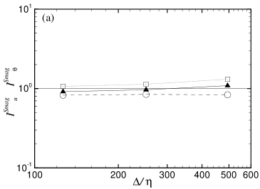
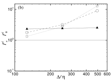
Figure 5: Isotropy ratios of components in SGS dissipations from models at $x_{2}/\ell=1.44$, as a function of filter scale: (a) eddy-diffusion models: $\circ$, $I_{u22}^{\mathrm{Smag}}$; $\square$, $I_{u12}^{\mathrm{Smag}}$; $\blacktriangle$, $I_{\theta}^{\mathrm{Smag}}$ (see Eq. 4); (b) nonlinear models: $\circ$, $I_{u22}^{\mathrm{nl}}$; $\square$, $I_{u12}^{\mathrm{nl}}$; $\blacktriangle$, $I_{\theta}^{\mathrm{nl}}$ (see Eq. 6).

The second modeling class to be considered here is the ‘nonlinear model’ or ‘tensor eddy-diffusion model’ (Leonard 1974, Clark, Ferziger & Reynolds 1979, Liu, Meneveau & Katz 1994, Leonard 1997, Borue & Orszag 1998 and Meneveau & Katz 2000). The nonlinear model reads as follows:

$$\tau_{ij}^{\mathrm{nl}}~{}=~{}C_{nl}\Delta^{2}\frac{\partial\widetilde{u}_{i}}{\partial x_{k}}\frac{\partial\widetilde{u}_{j}}{\partial x_{k}},~{}~{}~{}q_{j}^{\mathrm{nl}}~{}=~{}C_{{nl}_{\theta}}\Delta^{2}\frac{\partial\widetilde{\theta}}{\partial x_{k}}\frac{\partial\widetilde{u}_{j}}{\partial x_{k}},$$ (5)

where $C_{nl}$ and $C_{{nl}_{\theta}}$ are the nonlinear model coefficients. Therefore, the corresponding isotropy ratios from the nonlinear model are defined as follows:

$$I_{u22}^{\mathrm{nl}}\equiv\frac{\left<\frac{\partial\widetilde{u}_{2}}{\partial x_{k}}\frac{\partial\widetilde{u}_{2}}{\partial x_{k}}\widetilde{S}_{22}\right>}{\left<\frac{\partial\widetilde{u}_{1}}{\partial x_{k}}\frac{\partial\widetilde{u}_{1}}{\partial x_{k}}\widetilde{S}_{11}\right>},~{}~{}~{}I_{u12}^{\mathrm{nl}}\equiv\frac{\left<\frac{\partial\widetilde{u}_{1}}{\partial x_{k}}\frac{\partial\widetilde{u}_{2}}{\partial x_{k}}\widetilde{S}_{12}\right>}{\frac{3}{4}\left<\frac{\partial\widetilde{u}_{1}}{\partial x_{k}}\frac{\partial\widetilde{u}_{1}}{\partial x_{k}}\widetilde{S}_{11}\right>},~{}~{}~{}I_{\theta}^{\mathrm{nl}}\equiv\frac{\left<\frac{\partial\widetilde{\theta}}{\partial x_{k}}\frac{\partial\widetilde{u}_{2}}{\partial x_{k}}\widetilde{G}_{2}\right>}{\left<\frac{\partial\widetilde{\theta}}{\partial x_{k}}\frac{\partial\widetilde{u}_{1}}{\partial x_{k}}\widetilde{G}_{1}\right>},$$ (6)

where $k$ varies from 1 to 2 in the analysis of our 2D data.

The isotropy ratios of the SGS dissipations from the nonlinear model are shown in figure 5(b), as a function of filter scale. As is apparent in comparing with figure 4, the main features of anisotropy and filter-size dependence are correctly reproduced qualitatively. Quantitatively, the levels of anisotropy are overestimated. For instance, the level of anisotropy for the modeled SGS scalar-variance dissipation appears to stay near $I_{\theta}^{\mathrm{nl}}\sim 2.5$ as opposed to $I_{\theta}\sim 2$ for the real SGS scalar dissipation.

4 Summary and conclusions

In studying passive scalar statistics in a turbulent shear flow with a mean temperature gradient we focus on statistics of interest to subgrid modeling and large-eddy simulation. In order to obtain the filtered and subgrid velocities and temperatures, a probe array composed of four X-wire and four cold-wire sensors is used and two-dimensional box filtering in the streamwise and cross-wake directions is applied to the data. The isotropy ratios of the SGS kinetic energy and scalar-variance dissipations are investigated as function of position in the flow and as a function of filter scale. Both dissipations are isotropic independent of filter size near the centerline where there is no mean shear or scalar gradient. However, at locations with high gradient (and also further towards the outer wake regions), we find that the scalar-variance dissipation remains highly anisotropic, independent of filter size. Conversely, the kinetic energy dissipation tensor approaches isotropy as the filter size is decreased. A mechanistic explanation of the observed trends in terms of possible orientations of ramp and cliff structures is not evident to us at this time. The persistence of scalar anisotropy even at small scales is consistent with prior results for structure functions and gradient statistics of unfiltered turbulence (Mestayer 1982, Sreenivasan 1991, Warhaft 2000). Present results quantify the impact of this anisotropy on the interactions among large and small scales in the context of SGS modeling and LES.

We find that the predictions of eddy-diffusion models are much more isotropic than the real phenomenon. This may at first glance seem obvious since eddy-diffusion models are often invoked under the banner of isotropy. However, the present result does not arise from an explicit isotropy assumption built into the model, but because the resolved gradients have second-order statistics that are isotropic. For instance, if the scalar gradient tensor $\langle\tilde{G}_{i}\tilde{G}_{j}\rangle$ had been found to be anisotropic, it would have implied anisotropic behavior of the eddy-diffusion model’s predictions. Instead, the isotropy that exists in the filtered scalar gradients is incorrectly applied to model the anisotropic statistics of the SGS heat flux. The main problem for the eddy-diffusion model appears to be that it uses second-order statistics to model third-order statistics. Conversely, the anisotropy exists in the third-order moments that arise from the velocity and scalar product ($q_{i}$) multiplied by the scalar gradient ($\widetilde{G}_{j}$), but is not discernible in the second-order statistics of $\widetilde{G}_{j}$ alone (even when modulated by the strain-rate magnitude). The anisotropy is clearly discernible, however, in the third-order moments consisting of the filtered velocity gradients times scalar gradients squared that arise in the expression for modeled SGS dissipation of scalar-variance using the nonlinear model. These expressions are able to reproduce the detailed phase relationships among the velocity and scalar field that govern the SGS dissipation (cascade) of scalar variance. We remark that the overprediction of anisotropy by the nonlinear model (and its underprediction by the eddy-diffusion model) is reminiscent of the opposing trends of these two models documented in Liu et al. (1999) for rapidly strained turbulence in cold-flow. The opposing trends suggest that a linear combination of the two models, i.e. the ‘mixed model’, can be tuned to reproduce the correct amount of anisotropy (for a discussion of the application of mixed models in LES, see Meneveau & Katz 2000). However, note that the data for $I_{u12}$ and $I_{u22}$ at $\Delta/\eta=250$ and 125 do not provide clear justification for choosing the mixed over the non-linear model.

Finally, it is stressed that current results are obtained in a single flow for a single moderate Reynolds number. Even if the present evidence in figure 4 of an essentially scale-independent anisotropy for the scalar dissipation appears to be quite strong, the results could change in another flow, or at higher Reynolds numbers (we recall that according to Sreenivasan 1996, universal behavior for the scalar requires $Re_{\lambda}$ above 1000 or so). These considerations serve as motivation for further work in this area.