Three-dimensional numerical simulations of 1 GeV/Nucleon U92+ impact against atomic hydrogen
Abstract
The impact of 1 GeV/Nucleon U92+ projectiles against atomic hydrogen is studied by direct numerical resolution of the time-dependent non-relativistic wave-equation for the atomic electron on a three-dimensional Cartesian lattice. We employ the fully relativistic expressions to describe the electromagnetic fields created by the incident ion. The wave-equation for the atom interacting with the projectile is carefully derived from the time-dependent Dirac equation in order to retain all the relevant terms.
I Introduction
Atomic ionization by an electromagnetic wave, either incoherent or coherent, has been widely studied since the old times of Quantum Mechanics in many different situations. It is also obvious, but much less common in this context, to study ionization by the electromagnetic fields generated by a fast charged projectile passing nearby. In the case of a laser field, or any other electromagnetic wave, the field is a radiation field far from the sources, in other words, it is made of real photons [1]. However in case of a rapidly passing projectile, the field has different properties and it is just made of virtual photons.
That those virtual photons can ionize the atom is completely clear, but the ionization dynamics should be quite different from the laser field case. Recently, considerable interest has been devoted to this subject [2], both for single and multiple ionization of atoms with fast ions. However, very few experiments have been reported with relativistic incident ions. At the GSI in Darmstadt [3], experiments with relativistic incident ions have been performed. The GSI experiment studied the single and double ionization of helium by 1 GeV/Nucleon U92+ impact. As these authors state, the relativistic ion generates a sub-attosecond super-intense electromagnetic pulse.
Due to the geometry of the system (incident projectile and nucleus), there are no symmetries present except for a mirror symmetry along the plane defined by the projectile trajectory and the initial position of the nucleus. Therefore three-dimensional studies are needed and this is extremely difficult to be done ab initio for a two electron system. In the present paper we present a very realistic description of the (relativistic) ion-atom interaction but just for one-electron atoms. We compute the electron wave-function in a Cartesian three-dimensional lattice, taking into account the relativistic dynamics of the projectile.
Calculations in three-dimensional Cartesian grids have been shown to be a very good description for the collisions [4], with non-relativistic incident protons. The agreement with experimental results is remarkably good for the range of parameters considered. Collisions with antiprotons have been also investigated with these ab initio simulations [5, 6]. However these calculations are done in a context that is not able to describe the peculiar features of the electromagnetic fields (electric and magnetic fields) generated by the relativistically moving projectile. To our knowledge no previous studies have been done based on the numerical direct resolution of the wave-equation, in cases where the incident ion is relativistic.
A remarkable side consequence has been found. We need to describe a Lorentz transformed Coulomb field instead of the typical radiation fields studied in photo-ionization. For the correct quantum description of such interaction, it is necessary to include one extra term in the time-dependent Schrödinger equation. This term is missing in most of the studies on laser photo-ionization, that start from a time-dependent Schrödinger equation conceptually wrong.
The paper is organized as follows. In Sec. II we describe the electromagnetic fields created by a relativistically moving ion. In our calculations, we neglect both the recoil of the hydrogen nucleus so as the change in the trajectory of the ion: these approximations are justified in terms of classical simulations (Monte Carlo) in Sec. III. The derivation and discussion of the time-dependent wave-equation for the atomic system is described in Sec. IV. A detailed description of the integration algorithms and numerical techniques is also given. In Sec. V we establish the parameters of the calculations and we present the obtained numerical results. The final Section is devoted to conclusions.
II Electromagnetic fields
As our particular choice of the coordinates, to simplify the notation without loss of generality, we consider that the heavy ion projectile is moving in the plane in parallel direction to the x-axis. The hydrogen nucleus is initially at the origin and the projectile trajectory is , and . is the impact parameter (minimum distance to the nucleus in the trajectory of the ion). The notation is standard in relativity. The projectile is so heavy (, being the nucleon mass) and so energetic that we can perfectly assume that its trajectory is not affected by the atom. This point is discussed in Sec. III in terms of classical simulations.
It is not difficult to show [7] that the electric and magnetic fields created by such a relativistic projectile at an arbitrary point of space are,
| (1) |
and
| (2) |
with . indicates the projectile ion charge, that for the case studied here is =92.
These fields are generated by a scalar potential
| (3) |
and a vector potential
| (4) |
The velocity vector has only one component, . Therefore, and .
III Classical simulation
Although we give, in this paper, a quantum description of the dynamics of the atomic electron interacting with the ion, it is worth to start with a classical simulation of the three-body problem studied. For the considered parameters of the incident ion, it is almost trivial to perform classical Monte Carlo simulations for the motion of the projectile ion, the proton and the electron. The goal of such simulations is just to introduce the right approximations for the subsequent quantum description.
A few conclusions appear from the classical simulations for heavy projectiles (U92+) that move relativistically (1 GeV/Nucleon, or more). First, the projectile trajectory is not changed at the space scale and with the precision that we are interested in. Second, the hydrogen nucleus is accelerated after the collision with the projectile but the momentum transfer is negligible unless we consider impact parameters smaller than 0.1 a.u. We are not interested in head-on collisions, that could be relevant for nuclear physics.
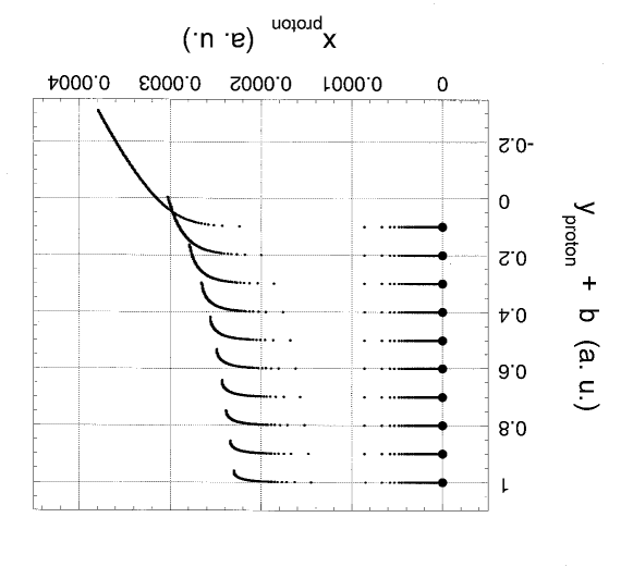
In Fig. 1 we represent the motion of the hydrogen nucleus for different values of the impact parameter (). The horizontal axis shows the motion in the longitudinal direction ( coordinate), and the vertical axis shows the motion in the transversal direction ( coordinate), where the impact parameter has been added for better observing all the curves. Both scales are in atomic units. The trajectories has been plotted since the incident projectile is placed at a.u. (marked with big circles) until it reaches a.u.
A result is clear: for the study of the ionization up to the level of accuracy we are interested in, it is fairly exact to consider that the projectile ion follows its trajectory unaltered. It is also reasonable, due to the short interaction time, to consider that the hydrogen nucleus remains unaltered at its initial position. Therefore only the electron motion needs to be described in detail. On the other side, the classical simulations indicate that the electron’s motion is essentially non-relativistic, except for extremely small impact parameters.
IV Time-dependent wave-equation
Because the electron is interacting with such time and space dependent scalar and vector potentials, it is worth to carefully describe the structure of the wave-equation. It is well known that the Dirac equation for an electron interacting with an arbitrary electromagnetic field and described with the scalar potential, , and the vector potential, , can be written as a second-oder differential equation [8]
| (5) |
where is the standard Dirac four-spinor, and and are matrices. The space and time dependence on the fields, potentials and wave-function has been removed for simplicity in the expressions. To describe the Coulomb potential of the hydrogen atom we have also included the term.
To move to the non-relativistic domain we start by neglecting the term, as it mixes particle and antiparticle states. We also neglect the coupling between spin and magnetic field, , because the degree of freedom of spin is not expected to play an important role in the dynamics of the electron, in the cases that we are considering. Now we can just consider a one-component wave-function
| (6) |
Expanding the square that includes the time derivative, and taking into account that the scalar potential can be time-dependent:
| (7) |
We now introduce explicitely the fast time oscillation,
| (8) |
and the wave-equation becomes,
| (9) | |||
| (10) |
so that we have eliminated the fast oscillation due to the mass term. The next step towards the non-relativistic wave-equation consists of neglecting the term, because the fast oscillations due to the mass term have been explicitly accounted for. Moreover it is consistent with the non-relativistic limit we are looking for to assume, . Thus the wave-equation is simplified to,
| (11) |
The term should not be eliminated because even when the modulus is very small compared with the electron’s rest mass, it is dephased due to the factor. Therefore it is necessary to keep this term,
| (12) |
It is worth to write this wave-equation in the form of a Hamiltonian system. This Hamiltonian has an extra term , that needs to be included in the time-dependent Schrödinger equation. This term is, however, fundamental for the validity of this non-relativistic equation for any scalar and vector potentials with arbitrary space-time dependences.
Expanding the term, and taking care of the non-commutability of and , one gets,
| (13) |
If we introduce the Lorentz condition for the scalar and vector potentials,
| (14) |
the wave-equation is heavily simplified,
| (15) |
Observe that this equation is different from the standard time-dependent Schrödinger equation, that considers the term : it includes the divergence of the vector potential but it does not include the very important term. Such equation is not general and can not be safely employed to describe the interaction with arbitrary electromagnetic fields. Only transversal electromagnetic fields can be accurately described. We have introduced this derivation prior to start computing the dynamics of the electron in order to clarify this point, that could become a source of error in the description of the system.
One final remark on the above equation. The fields that we describe with and , Eq. (3) and Eq. (4), are invariant under Lorentz transformations. The time-dependent Schrödinger equation is invariant under Galilean transformations due to its non-relativistic nature. However, Eq. (15) shows neither one nor the other kind of invariance. This formal inconsistency in our model is not important if the dynamics of the electron is non-relativistic (like in the cases that we are considering), and thus Lorentz transformations reduces to Galilean transformations (in the low velocity regime).
The final equation that we consider is:
| (16) | |||||
| (17) |
is the Coulomb potential. The electromagnetic potentials are given by Eqs. (3) and (4), and they already verify the Lorentz condition because they come from the Lorentz transform of a Coulomb potential.
We numerically solve Eq. (17) on a three-dimensional Cartesian lattice with a uniform grid spacing a.u. The lattice is taken in such a way that avoids the singularity in the origin by considering grid points at half integer times the grid spacing.
Our numerical technique is based on a symmetric splitting of the time-evolution operator so that the wave-function at a given time is calculated from the wave-function in the previous time step :
| (18) | |||||
| (19) | |||||
| (20) | |||||
| (21) |
We have defined the hamiltonian operators as follows:
| (22) | |||||
| (23) |
The exponentials are thus expressed in the Cayley unitary form [9], that preserves the norm of the wave-function, and a Crank-Nicholson scheme is employed to evaluate the space derivatives. Similar methods have been successfully employed to integrate the non dipole Schrödinger equation for the interaction of atoms with very intense laser fields [10].
The initial state for our calculations (the ground state of atomic hydrogen) is computed in a lattice with the imaginary time propagation method. The computed energy for this state is a.u.
Two different grid sizes have been employed to describe the ion-hydrogen collision, depending on the value of the impact parameter ():
| (24) |
Absorbers (a mask function) were employed at the integration boundaries in order to avoid reflections of the ionized population. The mask function has the form and it is applied over points along the edge of the grid. However, the interaction time is short enough to avoid a very large amount of population reaching the boundaries (absorbed population is always smaller that percent).
V Numerical results
In our calculations, the hydrogen nucleus is placed at the origin of the Cartesian coordinates. For the selected energy of the incident ion (1 GeV/Nucleon) the relativistic parameters are and . The U92+ nucleus is initially at a.u., and a.u. That choice of the initial value of is a good compromise between accuracy -due to the long range of the Coulomb potential- and a reasonable computer time. The electronic wave-function is propagated in time until the ion reaches a.u. ( a.u. is the final time). time iterations are employed, so that the ion covers a distance equal to the grid spacing ( a.u.) each time step ( a.u.). In order to avoid problems with the singularity of the Coulomb potential of the ion, the projectile moves equidistantly to the nearest points of the lattice.
We investigate the effect of the impact parameter in the dynamics of the atomic electron by varying (non-uniformly) from a.u. to a.u. We avoid smaller impact parameters because they contribute negligibly to electron ionization cross sections and they turn out to be relevant for ion-proton scattering (a physical situation out of the scope of the present paper).
We evaluate, during the time propagation, the projection of the wave function over the ground state to compute the total excitation probability (probability of finding population both in free states as in bound excited states), for each value of the impact parameter:
| (25) |
is the volume of the integration box.
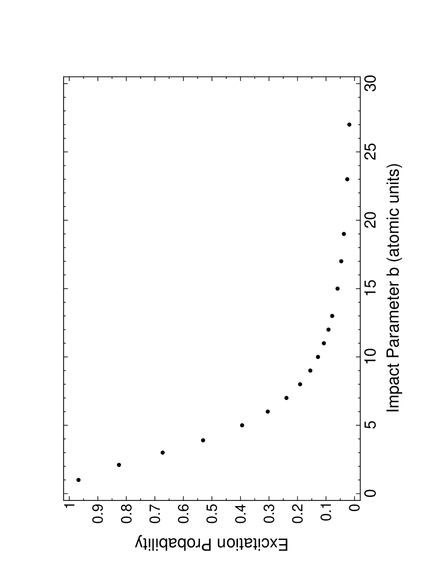
In Fig. 2 it is represented the computed values of for different impact parameters , at the final time . In fact, due to the fast motion of the ion, very few iterations after the ion has passed at the minimum distance to the nucleus (), the excitation probability remains approximately unchanged. From these values it is possible to estimate the total excitation cross section at the final time, defined as
| (26) |
We interpolate the excitation probability at the intermediate points with cubic-spline standard methods. The obtained value is cm2.
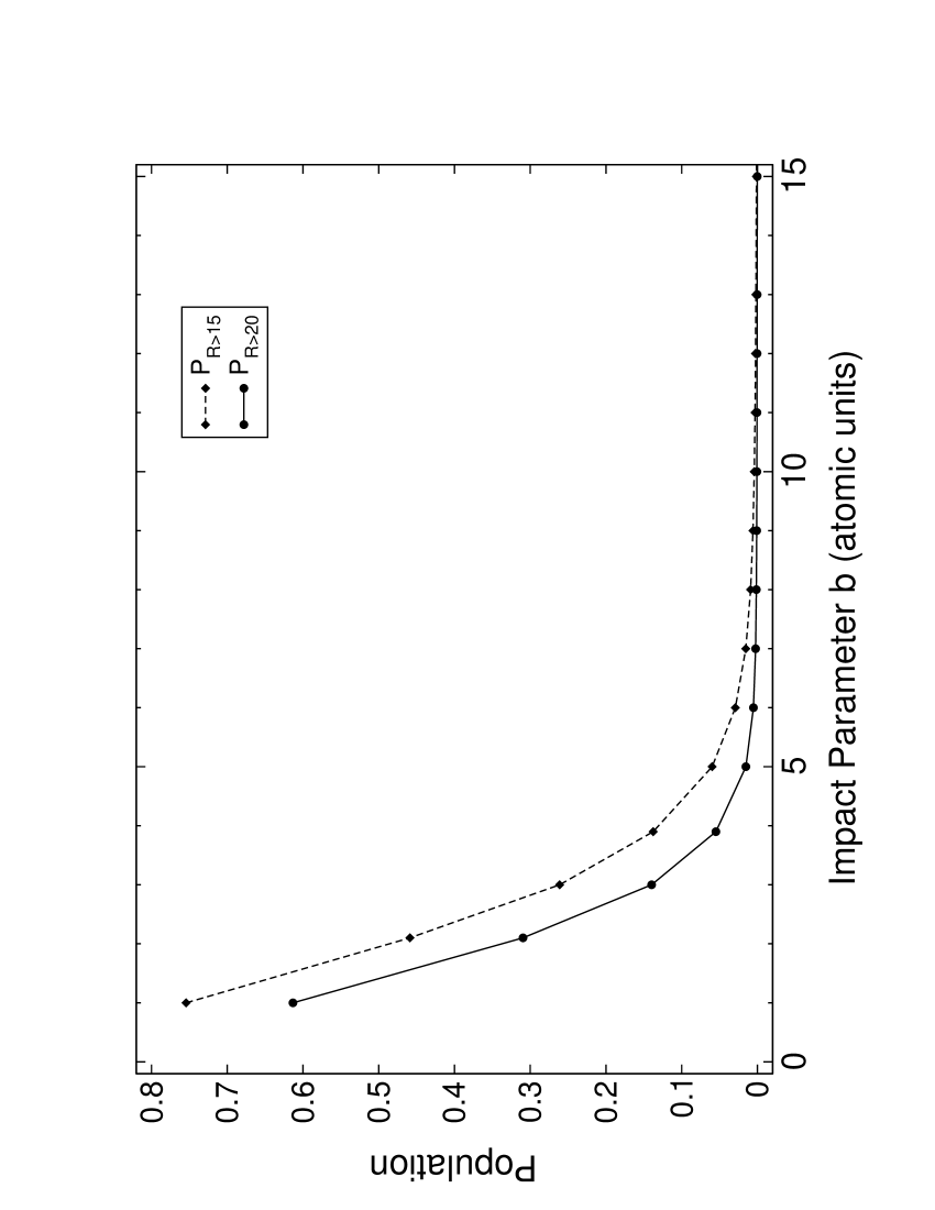
To gain insight into the dynamics of the electrons, we compute the population that remains, at any time of the interaction, at a distance to the nucleus greater than a.u. [] or greater than a.u. [], that can be regarded as ionized electrons. At the final time , both values of the population have been plotted in Fig. 3 in terms of the impact parameter . Dashed lines and diamonds corresponds to while solid lines and circles correspond to . Both curves sharply decreases from to a.u., so that very few electrons can be measured for larger impact parameters.
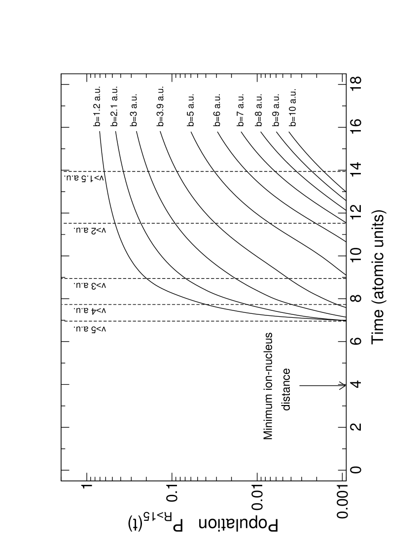
In Fig. 4 we plot the time evolution of the population , for different values of the impact parameter. The horizontal axis contain the interaction time in atomic units and the vertical axis the population . We may approximately know the velocity distribution of the ejected electrons, by simply assuming that ionization process occurs at the time when the ion is placed at the minimum distance to the nucleus [, and ]. In fact this is a good approximation due to the very high velocity of the projectile. The time at which the ion is placed at this minimum distance is marked with a vertical arrow. Vertical dashed lines indicate the minimum necessary velocity of the ejected electrons, , to reach the distance : a.u. (for ). Observe that no electrons are ejected with velocities greater that a.u. (). Thus, to employ the non-relativistic wave-equation is justified to describe the electron dynamics.
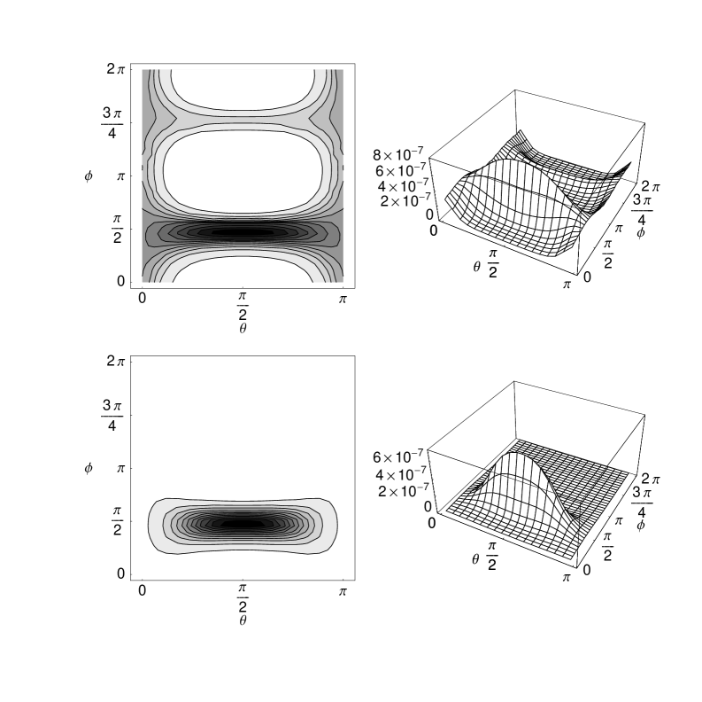
At the final time , we have also computed the angular distribution of the electrons. To do so we consider electrons placed between two spheres, i.e. electrons placed at a distance R from the nucleus such that with a.u. and These values of the radii mean that we are considering electrons ejected with approximated velocities in the range a.u. In Fig. 5 this angular distribution has been plotted for the impact parameter a.u. (plots at the top) and a.u. (plots at the bottom). The angular distribution per volume unit is defined by:
| (27) |
where we have defined:
| (28) | |||||
| (29) |
The spherical coordinates are defined in the standard form, , and . The angular step is rad. Plots on the left are contour plots with dark regions representing the maximum population. Contour lines are in linear scale. Plots on the right are surface plots, also in linear scale.
Observe the clear difference between both pairs of plots. For the impact parameter a.u., the peak of the ejected electrons is placed along the positive part of the -axis ( and ) but also appears a second peak along the negative part of the -axis ( and ). This second peak is a consequence of the fact that the ion crosses well over the electronic cloud. The minimum density of electrons are found along the -axis, the longitudinal direction, (, and , ). However for the impact parameter a.u. only the first peak can be observed: in this case the ion does not cross over the electronic cloud.
Finally, in Fig. 6 we plot the probability density at different times of the interaction with the ion, at the planes (plots at the top), (plots in the middle) and (plots at the bottom). The impact parameter is a.u. The column on the left corresponds to the time at which the ion is placed at the minimum distance to the nucleus []. The column in the middle is for a.u. ( a.u.) and the column on the right for a.u. ( a.u.). The contour lines are in logarithmic scale. In the frame in the first column, the effect of the incident ion can be observed as a distortion of the wave-packet. Once the projectile has passed, ionized population moves mainly along the transverse direction ( axis). The slight trembling in the lower contour lines that can be appreciated in a few frames, is due to spatial discretization effects and the non continuous evaluation of the trajectory of the ion.
VI Conclusions
We have presented very realistic three-dimensional numerical simulations to describe the collision of relativistic heavy ions against hydrogenic atoms. Our simulations are based on the ab initio integration of the time-dependent wave-equation derived from the non-relativistic limit of the Dirac equation, that is valid for arbitrary electrogmanetic potentials. This equation differs from the standard time-dependent Schrödinger equation in a term that includes the time derivative of the scalar potential: neglecting this term leads to a conceptually wrong formulation. The recoil of the ion and the motion of the atomic nucleus have been neglected in our simulations. We have employed a three-dimensional Cartesian grid to integrate the wave-equation. As results, we should point out that the probability of excitation of the atom sharply increases for impact parameters a.u. However, the ejection of fast electrons is only relevant for even smaller values of the impact parameter ( a.u.). The space distribution of such electrons is centered along the transversal direction. It is composed of one maximum (in the positive direction of the axis) even for short impact parameters ( a.u.). Only in collisions where the ion crosses over the electronic cloud a more complex structure appears.
ACKNOWLEDGMENTS
The authors gratefully acknowledge invaluable discussions with Luis Plaja. This work has been partially supported by the Spanish Dirección General de Enseñanza Superior e Investigación Científica (grant PB98-0268) and by the Junta de Castilla y León and Unión Europea, FSE (grant SA044/01). Computational work was carried out at the Linux cluster of the Optics Group in the Universidad de Salamanca.


REFERENCES
- [1] Reports on the interaction of atoms with very intense laser fields are, for instance, M. Protopapas, C.H. Keitel and P.L. Knight, Rep. Prog. Phys. 60, 389 (1997); C. J. Joachain, M. Dörr, and N. J. Kylstra, Adv. At. Mol. Opt. Phys. 42, 225 (2000).
- [2] J. Burgdörfer, L. R. Anderson, J. H. McGuire and T. Ishihara, Phys. Rev. A 50, 349 (1994); J. Wang, J. H. McGuire, J. Burgdörfer and Y. Qiu, Phys. Rev. Lett. 77, 1723 (1996); N. Stolterfoht, J.-Y. Chesnel, M. Grether, B. Skogvall, F. Frémont, D. Lecler, D. Hennecart, X. Husson, J. P. Grandin, B. Sulik, L. Gulyás and T. A. Tanis, Phys. Rev. Lett. 80, 4649 (1998).
- [3] R. Moshammer, W. Schmitt, J. Ullrich, H. Kollmus, A. Cassimi, R. Dörner, O. Jagutzki, R. Mann, R. E. Olson, H. T. Prinz, H. Schmidt-Böcking, and L. Spielberg, Phys. Rev. Lett. 79, 3621 (1997).
- [4] A. Kolakowska, M. S. Pindzola, F. Robicheaux, D. R. Schultz and J. C. Wells, Phys. Rev. A 58, 2872 (1998); D. R. Schultz, M. R. Strayer and J. C. Wells, Phys. Rev. Lett. 82, 3976 (1999); A. Kolakowska, M. S. Pindzola and D. R. Schultz, Phys. Rev. A 59, 3598 (1999).
- [5] D. R. Schultz, P. S. Krstic, C. O. Reinhold and J. C. Wells, Phys. Rev. Lett. 76, 2882 (1996); J. C. Wells, D. R. Schultz, P. Gavras and M. S. Pindzola, Phys. Rev. A 54, 593 (1996).
- [6] D. R. Schultz, J. C. Wells, P. S. Krstic and C. O. Reinhold, Phys. Rev. A 56, 3710 (1997).
- [7] Jackson J D, Classical Electrodynamics, (John Wiley and Sons, New York, 1998).
- [8] See for instance, L. I. Schiff, Quantum Mechanics, (McGraw-Hill, New York, 1968).
- [9] H. W. Press, S. A. Teukolsky, W. T. Vetterling and B. P. Flannery, Numerical Recipes in C, (Cambridge University Press, Cambridge, 1992).
- [10] J. R. Vázquez de Aldana and Luis Roso, Phys. Rev. A (2001) submitted.