Dynamic Model for LES Without Test Filtering: Quantifying the Accuracy of Taylor Series Approximations

Abstract

The dynamic model for large-eddy simulation (LES) of turbulent flows requires test filtering the resolved velocity fields in order to determine model coefficients. However, test filtering is costly to perform in large-eddy simulation of complex geometry flows, especially on unstructured grids. The objective of this work is to develop and test an approximate but less costly dynamic procedure which does not require test filtering. The proposed method is based on Taylor series expansions of the resolved velocity fields. Accuracy is governed by the derivative schemes used in the calculation and the number of terms considered in the approximation to the test filtering operator. The expansion is developed up to fourth order, and results are tested a priori based on direct numerical simulation data of forced isotropic turbulence in the context of the dynamic Smagorinsky model. The tests compare the dynamic Smagorinsky coefficient obtained from filtering with those obtained from application of the Taylor series expansion. They show that the expansion up to second order provides a reasonable approximation to the true dynamic coefficient (with errors on the order of about 5% for $c_{s}^{2}$), but that including higher-order terms does not necessarily lead to improvements in the results due to inherent limitations in accurately evaluating high-order derivatives. A posteriori tests using the Taylor series approximation in LES of forced isotropic turbulence and channel flow confirm that the Taylor series approximation yields accurate results for the dynamic coefficient. Moreover, the simulations are stable and yield accurate resolved velocity statistics.

1 Introduction

In large-eddy simulation (LES), the Navier–Stokes equations are filtered in an attempt to isolate the large-scale motion in a turbulent flow. The filtered equations contain the divergence of the sub-grid scale (SGS) stress,

$$\tau_{ij}=\widetilde{u_{i}u_{j}}-\widetilde{u}_{i}\widetilde{u}_{j},$$ (1)

where ($\tilde{\ }$) denotes a filtering operation. This filter, called the grid filter, is a convolution with the kernel $G_{\Delta}$,

$$\widetilde{f}(\vec{x})=\int\limits_{\mathbb{R}^{3}}f(\vec{x}^{\prime})G_{\Delta}(\vec{x},\vec{x}^{\prime})\,\D\vec{x}^{\prime},$$ (2)

which has a smoothing action on the scales smaller than $\Delta$. Analogous to the closure problem related to the Reynolds-averaged Navier–Stokes equations, the SGS stress $\tau_{ij}$ must be modeled using available filtered quantities. A variety of SGS models exist (Piomelli, 1999; Meneveau and Katz, 2000), but the results largely depend upon the choice of model coefficients, and the latter often have to be tuned from one flow regime to another. The dynamic procedure introduced by Germano et al. (1991) avoids such ad-hoc tuning. A crucial step in the dynamic procedure is using a filtering operation, called test filtering, to gather information about the smallest resolved scales. The test filtering operation, denoted by ($\bar{\ }$), is defined in a similar way to the grid filter, except the filter acts on a larger scale $\alpha\Delta$:

$$\overline{\widetilde{f}}(\vec{x})=\int\limits_{\mathbb{R}^{3}}\widetilde{f}(\vec{x}^{\prime})G_{\alpha\Delta}(\vec{x},\vec{x}^{\prime})\,\D\vec{x}^{\prime},\qquad(\alpha>1).$$ (3)

In this paper, we restrict attention to the dynamic formulation (Germano et al., 1991) of the Smagorinsky (Smagorinsky, 1963) eddy-viscosity model. It approximates the deviatoric part of the SGS stress by

$$\tau_{ij}-\frac{1}{3}\tau_{kk}\delta_{ij}=-2(c_{s}\Delta)^{2}|\widetilde{S}|\widetilde{S}_{ij},$$ (4)

where $c_{s}$ is the Smagorinsky constant, $\widetilde{S}_{ij}=\frac{1}{2}(\partial_{j}\widetilde{u}_{i}+\partial_{i}\widetilde{u}_{j})$ is the filtered rate of strain tensor, and $|\widetilde{S}|=(2\,\widetilde{S}_{ij}\widetilde{S}_{ij})^{1/2}$ is the filtered strain-rate magnitude. The expression for $c_{s}^{2}$, obtained by minimizing the mean square error in the Germano identity (see Germano et al., 1991; Lilly, 1992), $\mathcal{E}=\left\langle\left[L^{f}_{ij}-{\left(c_{s}^{f}\right)}^{2}M^{f}_{ij}\right]^{2}\right\rangle$, is

$$\left(c^{f}_{s}\right)^{2}=\frac{\langle L^{f}_{ij}M^{f}_{ij}\rangle}{\langle M^{f}_{k\ell}M^{f}_{k\ell}\rangle},$$ (5)

where the angle brackets denote an averaging operation (Ghosal et al., 1995),

$$L^{f}_{ij}=\overline{\widetilde{u}_{i}\widetilde{u}_{j}}-\overline{\widetilde{u}}_{i}\overline{\widetilde{u}}_{j}$$ (6)

is the resolved turbulent stress, and

$$M^{f}_{ij}=2\Delta^{2}\left[\overline{|\widetilde{S}|\widetilde{S}_{ij}}-\alpha^{2}|\overline{\widetilde{S}}|\overline{\widetilde{S}}_{ij}\right]$$ (7)

(the superscript “$f$” in both tensors refers to “filtering”—to be later contrasted to Taylor series approximations). In (7), for simplicity, we have put $\alpha$ in place of the ratio of the ‘compound’ filter length to the grid filter length, where ‘compound’ filter length is the effective length scale of the filter obtained by sequentially applying the grid and test filters. The error in doing so is tolerable for typical values of $\alpha$ and one can calculate the precise form of this ratio after choosing a specific type of test filter and assuming a form for the implicit grid filter. The reader is referred to Winckelmans et al. (1998) for further discussion. The averaging in (5) may be done over directions of statistical homogeneity (Germano et al., 1991), if any exist. In complex geometries without homogeneous directions, the Lagrangian dynamic model (Meneveau et al., 1996), which calculates time averages along pathlines, can be used. In the present work, only turbulence with statistically homogeneous directions will be considered for simplicity. Hence, spatial averaging is employed in all applications.

However, from a practical perspective, test filtering adds computational cost to LES. The cost is typically manageable when dealing with pseudo-spectral numerical methods, where filter operations can be performed in Fourier space. When using physical-space based test filtering approaches (e.g. in finite-difference or finite-volume codes with structured grids), the operation count depends upon the number of neighboring grid-points involved in the filtering. Najjar and Tafti (1996) give a discussion of the effects of using test filters with finite-difference approximations and implications for the dynamic Smagorinsky model. When dealing with complex-geometry flows, unstructured grids are often employed for which one must decide which neighboring nodes are involved in the filtering. Challenges also arise when seeking parallelization. These difficulties have somewhat limited the applicability of the dynamic model to LES of complex-geometry flows. Various filtering operators for unstructured grids have already been proposed and tested, in several papers by Jansen (1994, 1999). He discusses and compares several options, including derivative based filtering, and generalized top-hat filtering (Jansen, 1999). The generalized top-hat filter is a natural extension of the top-hat filter to unstructured grids by averaging over all elements that share a particular node. Filtering methods for complex geometries have also been discussed by Mullen and Fischer (1999).

The derivative-based filter approximates the function to be test filtered by expanding it locally in a Taylor series and truncating. This method is attractive because typical codes already have efficient methods in place to evaluate derivatives (as opposed to filtering, which is not typically needed in most existing codes). As reviewed in Meneveau and Katz (2000), the idea of expanding the local velocity field in a Taylor series has been used before in SGS modeling, mainly to simplify modeling terms for the similarity model and/or the Leonard stresses (Leonard, 1974; Clark et al., 1979; Liu et al., 1994; Winckelmans et al., 1998), and also in the context of so-called defiltering SGS models (Stolz and Adams, 1999; Kuerten et al., 1999). In the context of the dynamic Smagorinsky model, Taylor series expansion was originally suggested by Gao and O’Brien (1993) to analytically study the limit $\alpha\to 1$, but was not applied or extended in LES. As mentioned above, the derivative based filter (or Taylor series approach) was one of the options tested by Jansen (1999), although no detailed results are presented for this approach. Jansen has used generalized top-hat filtering in his dynamic LES of airfoil flow because this method has been found to be cheaper than the Taylor series method and yet gives similar accuracy (Jansen, 1999), in the context of his specific code. The derivative based method has also been used to perform a priori studies of the sensitivity of various SGS models to the type of test filtering employed (Sagaut and Grohens, 1999).

In the present paper we focus on the Taylor series method because it is a fairly general approach which can be formulated, studied, and tested in general, less code-specific terms. Section 2 describes the formulation of the approach, in which the dynamic Smagorinsky coefficient is expressed entirely in terms of derivatives of the resolved velocity field and no test filtering is required. The accuracy of this approach is tested both a priori (§ 3) as well as a posteriori in LES of two benchmark flows, namely forced isotropic turbulence and minimal channel flow (§ 4). Structured grids are used both for the direct numerical simulation (DNS) used in the a priori tests and in the LES runs, in order to allow us to make comparisons in a highly controlled and standard numerical environment. Basic conclusions are presented in § 5.

2 Formulation

Given a quantity $\widetilde{f}(\vec{x})$ (time dependence is implicit) that is to be test filtered, $\widetilde{f}(\vec{x}^{\prime})$ in Equation (3) (written for a homogeneous filter) is replaced with its Taylor series expansion about the point $\vec{x}$. This leads to simple integrations that are performed analytically. The result is (assuming uniform convergence)

$$\overline{\widetilde{f}}(\vec{x})=\sum_{n=0}^{\infty}\frac{(-1)^{n}}{n!}\left.\partial^{n}_{i_{1}\cdots i_{n}}\widetilde{f}\right|_{\vec{x}}\langle y_{i_{1}}\cdots y_{i_{n}}\rangle,\qquad\vec{y}=\vec{x}-\vec{x^{\prime}},$$ (8)

where now the angle brackets denote the operation of taking the mean with respect to a homogeneous filter $G_{\alpha\Delta}$, e. g.,

$$\langle y_{i_{1}}\cdots y_{i_{n}}\rangle=\int\limits_{\mathbb{R}^{3}}y_{i_{1}}\cdots y_{i_{n}}G_{\alpha\Delta}(\vec{y})\,\D\vec{y}.$$ (9)

For an isotropic filter, we write $G_{\alpha\Delta}(\vec{y})=G_{\alpha\Delta}(|\vec{y}|)$, and all terms with $n$ odd vanish, so that we can take $n=2m$. The choice of an isotropic filter also effects the remaining terms since they all become isotropic tensors. Since derivatives can only be calculated to a limited accuracy, and we are forced to truncate the Taylor series, this method yields an approximation to the filtering operation. By varying the number of terms used in the Taylor series, and the way derivatives are calculated, the accuracy of this approximation can be varied.

Here, a formulation based entirely on the Gaussian filter,

$$G^{\mathrm{Gauss}}_{\Delta}(\vec{y})=\left(\frac{6}{\pi\Delta^{2}}\right)^{3/2}\exp\left(-\frac{6|\vec{y}|^{2}}{\Delta^{2}}\right),$$ (10)

is given although the approach can be extended to any isotropic filter with finite moments (this excludes the spectral cutoff filter, which has infinite second moments). Additionally, up to second order only, the following is also valid for the box filter, since the second moments of the Gaussian and box filters are the same. This means that the rest of the development in this section, up to second order only, can also be applied when using the box filter. This fact is used later in §4.2, where the box filter is used to perform test filtering. Restricting attention to the Gaussian filter, the moments in (8) can easily be evaluated as

$$\langle y_{i_{1}}\cdots y_{i_{2m}}\rangle=\sum\langle y_{i_{k_{1}}}y_{i_{k_{2}}}\rangle\cdots\langle y_{i_{k_{2m-1}}}y_{i_{k_{2m}}}\rangle,$$ (11)

where the sum is over all $(2m)!/\left(2^{m}m!\right)$ ways of partitioning $\left\{i_{1},i_{2},\cdots,i_{2m}\right\}$ into pairs (Isserlis, 1918). Using the result

$$\langle y_{i}y_{j}\rangle=\frac{(\alpha\Delta)^{2}}{12}\delta_{ij},$$ (12)

we have

$$\left<y_{i_{1}}\cdots y_{i_{2m}}\right>=\frac{(\alpha\Delta)^{2m}}{12^{m}}\sum\delta_{i_{k_{1}}i_{k_{2}}}\cdots\delta_{i_{k_{2m-1}}i_{k_{2m}}}.$$ (13)

Using (13) in (8), we have

$$\overline{\widetilde{f}}(\vec{x})=\sum_{m=0}^{\infty}\frac{(\alpha\Delta)^{2m}}{24^{m}m!}\left(\nabla^{2}\right)^{m}\widetilde{f}(\vec{x}),$$ (14)

where $\left(\nabla^{2}\right)^{m}$ denotes $m$ applications of the Laplacian operator. This expression allows one to replace test filtered quantities that appear in the dynamic model by expressions involving resolved (grid-filtered) quantities and their derivatives.

Application of (14) to $\widetilde{u}_{i}$, $\widetilde{u}_{j}$, and $\widetilde{u}_{i}\widetilde{u}_{j}$ yields the approximation

$$L^{t}_{ij}=\frac{(\alpha\Delta)^{2}}{12}{\frac{\partial\widetilde{u}_{i}}{\partial x_{k}}\frac{\partial\widetilde{u}_{j}}{\partial x_{k}}}+\frac{(\alpha\Delta)^{4}}{288}\left[\frac{\partial\widetilde{u}_{i}}{\partial x_{k}}\frac{\partial}{\partial x_{k}}\left(\frac{\partial^{2}\widetilde{u}_{j}}{\partial x_{m}^{2}}\right)+\frac{\partial^{2}\widetilde{u}_{i}}{\partial x_{k}\partial x_{\ell}}\frac{\partial^{2}\widetilde{u}_{j}}{\partial x_{k}\partial x_{\ell}}+\frac{\partial}{\partial x_{k}}\left(\frac{\partial^{2}\widetilde{u}_{i}}{\partial x_{m}^{2}}\right)\frac{\partial\widetilde{u}_{j}}{\partial x_{k}}\right]+O(\Delta^{6}).$$ (15)

Here, the terms involving derivatives of the product $\widetilde{u}_{i}\widetilde{u}_{j}$ have been expanded to take advantage of the favorable cancellation. The superscript “$t$” stands for “Taylor series approximation”. Similarly, after applying (14) to $\widetilde{S}_{ij}$ and $|\widetilde{S}|\widetilde{S}_{ij}$, we can calculate an approximation for $M_{ij}$,

$$M^{t}_{ij} = 2\Delta^{2}\left\{\left(|\widetilde{S}|\widetilde{S}_{ij}-\alpha^{2}|{\widetilde{S}^{t}}|\widetilde{S}_{ij}\right)+\frac{(\alpha\Delta)^{2}}{24}\left[{\partial_{m}^{2}}\left(|\widetilde{S}|\widetilde{S}_{ij}\right)-\alpha^{2}|{\widetilde{S}}^{t}|{\partial_{m}^{2}}\widetilde{S}_{ij}\right]\right.$$ (16)

$$\left.+\frac{(\alpha\Delta)^{4}}{1152}\left[\nabla^{4}\left(|\widetilde{S}|\widetilde{S}_{ij}\right)-\alpha^{2}|{\widetilde{S}}^{t}|\nabla^{4}\widetilde{S}_{ij}\right]+O(\Delta^{6})\right\},$$

where $|{\widetilde{S}}^{t}|$ is the derivative-based approximation to $|\overline{\widetilde{S}}|$,

$$|{\widetilde{S}}^{t}|=\left[2\left(\widetilde{S}_{ij}+\frac{\left(\alpha\Delta\right)^{2}}{24}{\partial_{m}^{2}}\widetilde{S}_{ij}+\frac{\left(\alpha\Delta\right)^{4}}{1152}\nabla^{4}\widetilde{S}_{ij}+O(\Delta^{6})\right)^{2}\right]^{1/2}.$$ (17)

Here, the derivatives of products have not been expanded, since no cancellation in the terms of $M^{t}_{ij}$ occurs. The dynamic coefficient $c^{t}_{s}$ can then be computed as before by evaluating tensor contractions and averaging over homogeneous directions. For example, below we will make frequent use of the case where only the $2^{\mathrm{nd}}$ order expansions are kept, so that we have

$${c^{t}_{s}}^{2}=\frac{\alpha^{2}}{24}\frac{\left<({\partial_{k}\widetilde{u}_{i}\partial_{k}\widetilde{u}_{j}})\left(\left(|\widetilde{S}|-\alpha^{2}|{\widetilde{S}}^{t}|\right)\widetilde{S}_{ij}+\frac{(\alpha\Delta)^{2}}{24}\left[{\partial_{m}^{2}}\left(|\widetilde{S}|\widetilde{S}_{ij}\right)-\alpha^{2}|{\widetilde{S}}^{t}|{\partial_{m}^{2}}\widetilde{S}_{ij}\right]\right)\right>}{\left<\left(\left(|\widetilde{S}|-\alpha^{2}|{\widetilde{S}}^{t}|\right)\widetilde{S}_{\ell n}+\frac{(\alpha\Delta)^{2}}{24}\left[{\partial_{m}^{2}}\left(|\widetilde{S}|\widetilde{S}_{\ell n}\right)-\alpha^{2}|{\widetilde{S}}^{t}|{\partial_{m}^{2}}\widetilde{S}_{\ell n}\right]\right)^{2}\right>},$$ (18)

with

$$|{\widetilde{S}}^{t}|=\left[2\left(\widetilde{S}_{ij}+\frac{\left(\alpha\Delta\right)^{2}}{24}{\partial_{m}^{2}}\widetilde{S}_{ij}\right)^{2}\right]^{1/2}.$$ (19)

In the case of isotropic turbulence, the test filtering is done in three dimensions, so that the values of the indices $k$ and $m$ in (18) are $1$, $2$, $3$, and the averaging in the numerator and denominator is volume averaging. However, in the case of channel flow, in order to approximate planar (in $x$-$z$ planes) instead of volumetric filtering, the Laplacian term in the expansion of (8) only contains derivatives in the $x$ and $z$ directions (i. e. the indices $k$ and $m$ in (18) and (19) only cycle over the two values $k=1$, $3$ and $m=1$,$3$). Additionally, in the channel flow case, plane averaging of the numerator and denominator of (18) is performed in the $x$-$z$ planes.

3 A priori tests

3.1 Methods

The a priori tests are done using a $128^{3}$ DNS database of forced isotropic turbulence at $R_{\lambda}\approx 94$, produced using the same pseudo-spectral algorithm as in Cerutti and Meneveau (1998). The grid filter size, $\Delta$, is chosen to be the grid spacing of a $32^{3}$ grid, and corresponds to $\Delta/\eta\sim 9$, where $\eta$ is the Kolmogorov scale. To perform the data analysis on the $32^{3}$ grid, the $128^{3}$ DNS data is grid filtered (using the Gaussian filter) and stored back on the DNS grid. Then, the grid-filtered velocity is filtered using a spectral cutoff filter of width $\Delta$ (the same as the $32^{3}$ grid spacing) so that no aliasing occurs when transferring the velocity to the $32^{3}$ grid. The grid-filtered velocity, on the coarse grid, is then used to calculate the filtered rate of strain tensor using finite differences. The model coefficient $c_{s}^{2}$ is calculated using the approximations (15), (16), and (17), and is compared to values obtained by explicitly applying a test filter. The series (14) must be truncated, so here two levels of accuracy are considered: second order and fourth order. The second order approximation (denoted as $T=2$) is obtained by keeping terms $O(\Delta^{2})$ and lower in (14), so only the first term in (15), and only the first two terms inside the curly braces in (16) are kept. The fourth order approximation (denoted as $T=4$) is obtained in an analogous way and contains all of the explicitly shown terms in (15) and (16).

At both levels of accuracy, all of the derivatives required to implement the derivative-based test filtering are initially calculated using centered finite differences accurate to second order (denoted as $D=2$). These derivatives could be calculated spectrally, however the goal here is to examine how the derivative-based method performs when derivatives are calculated as they would be in a complex geometry situation. In an attempt to separate the errors due to truncating the series (14) and finite differencing errors, fourth order finite differences (denoted as $D=4$) are also tried for calculating derivatives. This allows one to keep the filter size constant while the accuracy of the finite differences is changed.

A coarse $32^{3}$ grid is used to store the grid-filtered velocity during the a priori test, so that all subsequent calculations would be the same as if a LES was actually being performed. This is also consistent with the choice of grid filter size. The ratio of the widths associated with the test filter and the grid filter, $\alpha$, is varied between $2$, $3$, and $4$, though in this study, the most attention is given to the common choice $\alpha=2$.

Finally, the approximations (15) and (16) are calculated to the desired level of accuracy and the results are used in (5) to calculate $c_{s}^{2}$. Spatial averaging is employed in (5) because of the spatial homogeneity of the velocity field under consideration. Note that since (15) and (16) contain products of velocity components, they also contain aliasing errors. However, these were not removed since it is assumed that methods to do so may not be available during a typical LES of a complex geometry flow.

3.2 Results

The results obtained from using the Taylor series approximations are compared to those obtained by performing the classical test filtering. The comparison is based on scatter plots of tensor element values for some representative cases, and on correlation coefficients and normalized mean square errors among individual tensor elements. The correlation coefficient for a given tensor element is defined as

$$\rho(L^{t}_{mn},L^{f}_{mn})=\frac{\left<L^{t}_{mn}L^{f}_{mn}\right>-\left<L^{t}_{mn}\right>\left<L^{f}_{mn}\right>}{\left[\left(\left<{L^{t}_{mn}}^{2}\right>-\left<L^{t}_{mn}\right>^{2}\right)~{}\left(\left<{L^{f}_{mn}}^{2}\right>-\left<{L^{f}_{mn}}\right>^{2}\right)\right]^{1/2}}$$ (20)

(no summation over indices), and similarly for the $M_{ij}$ tensor elements. In order to also quantify the agreement among the magnitudes of the tensors, we compute the normalized square error (Liu et al., 1999) defined as

$$\mathcal{E}(L^{t}_{mn},L^{f}_{mn})=\frac{\langle(L^{t}_{mn}-L^{f}_{mn})^{2}\rangle}{\langle(L^{f}_{mn})^{2}\rangle},$$ (21)

and similarly for the $M_{ij}$. Also the dynamic coefficient $c_{s}^{2}$ is evaluated by averaging the tensor contractions, and the relative error in $c_{s}^{2}$ is obtained.

3.2.1 Second order approximation

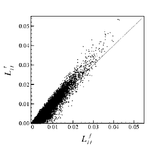
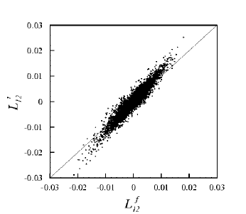
(a) (b)

Figure 1: Scatter plot of typical components of $L_{ij}$ evaluated using the Taylor series approach compared to the classical filter-based approach, for the case $\alpha=2$ with the $2^{\mathrm{nd}}$ order approximation ($T=2$). (a) shows $L_{11}$ while (b) shows $L_{12}$.

In this section, the results obtained by using the second order approximation ($T=2$) and second order finite differencing ($D=2$) are presented. Here, the parameter $\alpha$ is fixed at the common value of 2; effects of varying $\alpha$ are discussed in § 3.2.5. First, we compare the results for the components $L_{ij}$ obtained using the two methods. Scatter plots comparing the $2^{\mathrm{nd}}$ order approximation to the exact (filter-based) results are shown in Figure 1 for a diagonal and an off-diagonal component of $L_{ij}$. Both plots indicate that the $2^{\mathrm{nd}}$ order approximation is overall quite good, but has a tendency to under-estimate the magnitude of the $L$-components for small $|L_{ij}|$, but over-estimates the magnitude at larger $|L_{ij}|$.

As shown in the first column of Table 1, the $2^{\mathrm{nd}}$ order approximation is well correlated ($\rho\sim 0.95$) with the exact results, and the normalized square error between the two is $\sim 6\%$ for diagonal terms and $\sim 15\%$ for off-diagonal terms.

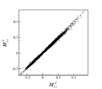
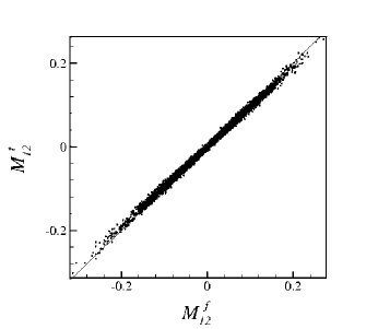
(a) (b)

Figure 2: Same as Figure 1, but for the tensor $M_{ij}$.(a) shows $M_{11}$ while (b) shows $M_{12}$.

Scatter plots of components of $M_{ij}$ obtained using the $2^{\mathrm{nd}}$ order approximation and the exact results are shown in Figure 2, from which it can be seen that the approximation is very good. As shown in Table 1, the $2^{\mathrm{nd}}$ order approximation for the $M_{ij}$ is very highly correlated with the exact values, with $\rho\sim 0.99$. The normalized mean square is significantly lower than it was for the $L_{ij}$, being $\sim 1\%$ for diagonal terms and $\sim 0.5\%$ for off-diagonal terms.

Using the approximate and exact results for $L_{ij}$ and $M_{ij}$ in Equation (5), and using volume averaging gives the values of $c_{s}^{2}$ shown in the last entries of Table 1. The relative error in $c_{s}^{2}$ obtained by using the $2^{\mathrm{nd}}$ order approximation is $\sim 5\%$. Since the value of the coefficient obtained in the present work is essentially the same as for the standard filtering approach, the dissipation characteristics will be the same as for the standard filter-based dynamic model.

3.2.2 Fourth order approximation

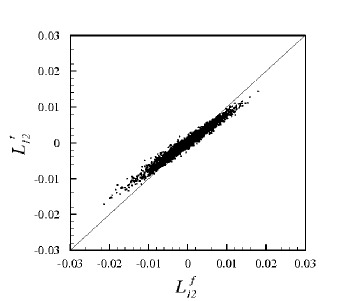
(a) (b)

Figure 3: Same as Figure 1 for the case $\alpha=2$, but now with the $4^{\mathrm{th}}$ order approximation ($T=4$). (a) shows $L_{11}$ while (b) shows $L_{12}$.

To answer the question of whether one can improve on the $5\%$ relative error of the $2^{\mathrm{nd}}$ order approximation by including higher order terms, a priori tests are done with the $4^{\mathrm{th}}$ order approximation ($T=4$, but still $D=2$). As in the $2^{\mathrm{nd}}$ order case above, we fix $\alpha=2$ here. Beginning with the components of $L_{ij}$, the scatter plots in Figure 3 show that the $4^{\mathrm{th}}$ order approximation tends to under-estimate the magnitude of the components of $L_{ij}$. Despite this, the correlation coefficient between the $4^{\mathrm{th}}$ order and exact results, shown in the second column of Table 1 to be $\sim 0.98$, is higher than it was between the $2^{\mathrm{nd}}$ order and exact results. Additionally, the normalized square error between the approximation and exact results for the $L_{ij}$, also in Table 1, is lower overall with an improvement in the off-diagonal terms outweighing a slight increase in the error of the diagonal terms. Note that with the use of the $4^{\mathrm{th}}$ order approximation, there is no longer a large discrepancy between the diagonal and off-diagonal terms, as was observed when the $2^{\mathrm{nd}}$ order approximation was used, as the normalized square error is $\sim 7\%$.

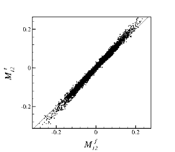
(a) (b)

Figure 4: Same as in Figure 2 using the the $4^{\mathrm{th}}$ order approximation ($T=4$). (a) shows $M_{11}$ while (b) shows $M_{12}$.

For $M_{ij}$, Figure 4 shows scatter plots obtained with the $4^{\mathrm{th}}$ order approximation, which now shows a slight tendency to over-estimate the magnitude of $M_{ij}$. The correlation coefficient is seen in table 1 to remain high, at $\sim 0.99$. However, the normalized square error for the $M_{ij}$ components is increased significantly to $\sim 3\%$ for both diagonal and off-diagonal terms by using the $4^{\mathrm{th}}$ order approximation. This is an increase from $1\%$ for diagonal terms and $0.5\%$ from the off-diagonal terms, which were obtained with the $2^{\mathrm{nd}}$ order approximation. As a result, the value of $c_{s}^{2}$ obtained with the $4^{\mathrm{th}}$ order approximation has a relative error of $\sim 27\%$. This is significantly worse than the results obtained using the $2^{\mathrm{nd}}$ order approximation.

There are two likely reasons why the $4^{\mathrm{th}}$ order approximation gives inferior results. The first is that the finite difference errors in the $2^{\mathrm{nd}}$ order terms are swamping the $4^{\mathrm{th}}$ order correction. In other words, due to the second-order finite differencing ($D=2$), the error in $\partial_{k}\widetilde{u}_{i}\partial_{k}\widetilde{u}_{j}$ in Equation 15 is $O(\Delta^{4})$—the same order as the $4^{\mathrm{th}}$ order correction. The second possible reason is that the filtered velocity field is simply not smooth enough to allow reliable calculation of high order derivatives through finite differencing. This issue is an inherent, well-known difficulty associated with LES velocity fields that have a Kolmogorov energy spectrum. Even after removing some energy near the grid-scale through the implicit grid filter, gradients are still dominated by modes very near the scale $\Delta$. Also note that the main problems seem to be associated with the error in the $4^{\mathrm{th}}$ order $M_{ij}$ terms, which contain the highest order velocity derivatives. These two possibilities are examined in more detail below.

3.2.3 Higher order derivative scheme

To check the possibility of whether the truncation error from the $O(\Delta^{2})$ finite differences is swamping the $4^{\mathrm{th}}$ order correction, more a priori tests were done using $O(\Delta^{4})$ finite differences to evaluate the $2^{\mathrm{nd}}$ order terms. This ensures that the finite difference truncation error from the $2^{\mathrm{nd}}$ order terms is now of higher order than the $4^{\mathrm{th}}$ order correction terms. To compare the relative importance of finite differencing error and the error associated with truncation in the Taylor series method, we consider the form of the leading error terms. This is done in one dimension only for simplicity. In the case $T=D=2$, the expansion with finite differences is

$$\overline{\widetilde{f}}(x)=\widetilde{f}(x)+\frac{(\alpha\Delta)^{2}}{24}\left(\widetilde{f}^{\prime\prime}(x)\right)_{fd}+{\alpha^{2}\Delta^{4}}\left(\frac{\alpha^{2}-2}{1152}\right)\left(\widetilde{f}^{iv}(x)\right)_{fd}+O(\Delta^{6}),$$ (22)

where the subscript $fd$ refers to derivatives calculated with centered finite differences, e.g. $\left(\widetilde{f}^{\prime\prime}(x)\right)_{fd}=(\widetilde{f}(x+\Delta)-2\widetilde{f}(x)+\widetilde{f}(x-\Delta))/\Delta^{2}$. In the case $T=4$, $D=2$, the leading error term is the $2/1152$ part of the coefficient of $\widetilde{f}^{iv}$ in the above expression, which is of the same order (in $\Delta$) as the fourth order term in the approximation to the test filter (i.e. the $\alpha^{2}/1152$ part of the coefficient of $\widetilde{f}^{iv}$). In particular, when $\alpha=2$ the finite differencing error is smaller but comparable to the fourth order correction term in the Taylor series expansion for the test filtered quantities.

With $D=4$, the expansion becomes

$$\overline{\widetilde{f}}(x)=\widetilde{f}(x)+\frac{(\alpha\Delta)^{2}}{24}\left(\widetilde{f}^{\prime\prime}(x)\right)_{fd}+\frac{(\alpha\Delta)^{4}}{1152}\left(\widetilde{f}^{iv}(x)\right)_{fd}+\alpha^{2}\Delta^{6}\left(\frac{5\alpha^{4}+192}{414720}\right)\left(\widetilde{f}^{vi}(x)\right)_{fd}+O(\Delta^{8}).$$ (23)

In the case $T=2$, $D=4$, we see that the leading error term is simply the fourth order correction term in the Taylor series expansion of the test filtering operator (the $(\alpha\Delta)^{4}/1152$ term). While in the case $T=D=4$, the leading error term is of higher order than the fourth order correction in the expansion of the test filtering operator (it is $\propto\Delta^{6}$). When $\alpha=2$, the finite difference error is larger, though of the same order of magnitude as the correction term for the test filter expansion.

The results for the $L_{ij}$ and $M_{ij}$ components, again for $\alpha=2$, are summarized in the third and fourth columns of Table 1. For the $2^{\mathrm{nd}}$ order approximation, although the correlation coefficients remain nearly the same as when the $2^{\mathrm{nd}}$ order finite differences were used, the normalized square error for $L_{ij}$ shows a significant increase, while it shows a smaller increase for $M_{ij}$. The resulting error in $c_{s}^{2}$ for the $2^{\mathrm{nd}}$ order approximation with $4^{\mathrm{th}}$ order finite differences is much larger ($37\%$) than when $2^{\mathrm{nd}}$ order finite differences are used. When the $4^{\mathrm{th}}$ order correction terms are included, evaluated with $4^{\mathrm{th}}$ order finite differences, the correlation coefficients for the $L_{ij}$ and $M_{ij}$ components do not change significantly. In contrast, the normalized square error for the $L_{ij}$ obtained with the $4^{\mathrm{th}}$ order approximation and $4^{\mathrm{th}}$ order differences is decreased significantly from both the $2^{\mathrm{nd}}$ order case with the $4^{\mathrm{th}}$ order finite differences and the $4^{\mathrm{th}}$ order case with only $2^{\mathrm{nd}}$ order finite differences. The normalized square errors for the $M_{ij}$ calculated using $4^{\mathrm{th}}$ order finite differences are increased from both the $2^{\mathrm{nd}}$ order approximation with $4^{\mathrm{th}}$ order finite differences, and the $4^{\mathrm{th}}$ order approximation with $2^{\mathrm{nd}}$ order finite differences. This shows that use of $O(\Delta^{4})$ finite differences can reduce error in using the $4^{\mathrm{th}}$ order approximation, but overall the results are not as good as when just $2^{\mathrm{nd}}$ order finite differences are used to implement the $2^{\mathrm{nd}}$ order approximation. Since the leading error term in (23) is at higher than fourth order, the above analysis of the error terms does not clearly explain the worsening of results in going from $T=D=2$ to $T=D=4$. A more intuitive analysis based on the roughness of the underlying velocity fields is given in the following section (§ 3.2.4).

3.2.4 Effects of smoothness

As a check to see under what conditions the $4^{\mathrm{th}}$ order approximation does give better results than the $2^{\mathrm{nd}}$ order approximation, the a priori tests are repeated with velocity fields of varying smoothness. A smoother velocity field allows more accurate calculation of high order derivatives, and also yields smaller errors in truncating the Taylor series. As a simple way to adjust the smoothness of the velocity field, an additional Gaussian filter is applied to the DNS data before performing the a priori tests. The width of this additional filter, or prefilter, is varied between $\Delta$ and $8\Delta$. This analysis is done here only to illustrate trends and is not proposed as a practical method in a simulation where we wish to avoid the need for filtering in the first place.

The results obtained with the prefilter width set to $4\Delta$ are summarized in the fifth column of Table 1. When $2^{\mathrm{nd}}$ order finite differences are used, it is seen that the normalized mean square error is increased for some components by going from the $2^{\mathrm{nd}}$ order approximation to the $4^{\mathrm{th}}$ order approximation. The relative error in $c_{s}^{2}$ is still higher for the $4^{\mathrm{th}}$ order approximation. The results obtained by using both $4^{\mathrm{th}}$ order finite differences and prefiltering are shown in the sixth column of Table 1. In this case, the normalized mean square error for the $L_{ij}$ components is decreased, while the results are mixed for the $M_{ij}$. The final value of $c_{s}^{2}$, as seen in Table 1 in this case does show an improvement in going from the $2^{\mathrm{nd}}$ order approximation to the $4^{\mathrm{th}}$ order approximation. This trend becomes more pronounced as the size of the prefilter is increased further. It is important to note that the resulting coefficients should not be compared to those obtained without prefiltering, because the velocity field in this case is actually different (it has been artificially smoothed out by the prefilter).

We conclude that only when the velocity field is very smooth does the use of the $4^{\mathrm{th}}$ order approximation yield more accurate results. However, this is not typically the case as LES fields are inherently somewhat rough. This result suggests that under typical circumstances, the $4^{\mathrm{th}}$ order approximation will yield poor results when compared to the $2^{\mathrm{nd}}$ order approximation.

3.2.5 Effect of varying $\alpha$

To examine how the size of the test filter affects the accuracy of the derivative based method, a priori tests are done with $\alpha=3$ and $4$, in addition to the base case of $\alpha=2$ discussed above. The derivatives in these tests are calculated using $2^{\mathrm{nd}}$ order finite differences and keeping the truncation to the second-order (i. e. $D=2$ and $T=2$). Since the derivative based method is based on truncating a Taylor series, one expects that the method will give better results for smaller values of $\alpha$, for a given $\Delta$. The correlation coefficients and normalized square errors for $L_{ij}$ and $M_{ij}$ are shown in the last two columns of Table 1. For $\alpha=3$, the correlation coefficients for $L_{ij}$ and $M_{ij}$ are decreased from their values obtained with $\alpha=2$. The normalized square error of the $L_{ij}$ obtained for the $2^{\mathrm{nd}}$ order approximation with $\alpha=3$ are increased dramatically over those obtained with $\alpha=2$, especially the off-diagonal terms, which show errors $\sim 120\%$. For the $M_{ij}$, the error obtained with the $2^{\mathrm{nd}}$ order approximation also shows a large increase in error compared to the case $\alpha=2$. The final results for $c_{s}^{2}$ are given in Table 1, and they show that the case $\alpha=3$ has a $6.41\%$ relative error. Considering the errors in the individual components of $L_{ij}$ and $M_{ij}$, this result is surprisingly good, but is most likely due to fortuitous cancellation of errors.

As seen in the last column in Table 1, for $\alpha=4$ the correlation coefficients for the $L_{ij}$ are decreased from the $\alpha=2$ and $\alpha=3$ cases. The correlation coefficients for the $M_{ij}$ are also decreased when choosing $\alpha=4$. The mean square error for both the $L_{ij}$ and the $M_{ij}$ is increased significantly in the $\alpha=4$ case. The error for $c_{s}^{2}$ obtained with $\alpha=4$ is seen to be very large. Analysis of the higher-order case ($T=4$, not shown) yields even larger errors. These a priori tests show that the Taylor series approximation to test filtering yields unsatisfactory results for $\alpha\gtrsim 3$ in this isotropic turbulent flow.

4 A posteriori tests

As a complement to the results of the a priori tests, a posteriori tests are used to compare the Taylor series based dynamic model to the traditional method based on test filtering. The tests are done by performing LES of both forced isotropic turbulence and channel flow. Since the best results in the a priori tests were obtained by truncating the Taylor series expansions at second order, all a posteriori tests are done using $T=2$ and $D=2$.

4.1 LES of Forced Isotropic Turbulence

To test the derivative-based method in isotropic turbulence, the pseudo-spectral DNS code is modified to perform LES on a $64^{3}$ grid. This includes adding a $3/2$-rule dealiasing procedure, which is applied only to the nonlinear term in the filtered Navier-Stokes equations ($\widetilde{\vec{u}}\times\widetilde{\vec{\omega}}$) and not the SGS stress term. This is done because the nonlinear term is known to be exact, while the SGS term is already an approximation. In addition, the type of nonlinearity contained in the SGS stress term is not completely removed by standard dealiasing procedures such as the $3/2$-rule or random phase shifts. Simulations are forced with a constant energy injection rate (as in Cerutti and Meneveau, 1998) of $\varepsilon=0.0007$, the molecular viscosity is $\nu=10^{-6}$, and the domain is of length $L=2\pi$. At statistical steady state, the Taylor-scale Reynolds number of the flow is $R_{\lambda}\approx 2100$. Simulations using both exact test filtering and the Taylor series based method are performed. As with the a priori tests, a Gaussian test filter is used at scale $2\Delta$ (corresponding to $\alpha=2$). The exact test filtering is done in Fourier space, while the Taylor series method uses second order finite differences to calculate all of the derivatives associated with the dynamic procedure. The initial condition is a random field with a $k^{-5/3}$ spectrum and random phases. Volume averaging is used in this spatially homogeneous flow.

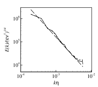
(a) (b)

Figure 5: Results from a posteriori tests in LES of forced isotropic turbulence on a $64^{3}$ domain with $R_{\lambda}\approx 2100$. (a) time evolution of dynamic Smagorinsky coefficients. Solid line: derivative-based, dashed line: test-filter based. (b) radial energy spectra. Solid line: derivative-based, dashed line: test-filter based dynamic model, long dashed line: normalized Kolmogorov spectrum $c_{K}(k\eta)^{-5/3}$ with $c_{K}=1.6$.

Figure 5(a) shows the time evolution of $c_{s}$ for exact test filtering and the derivative based approach. Although the derivative based method consistently gives a value of $c_{s}$ roughly $5$ % higher than the exact method (in contrast to the a-priori tests), both methods relax from the initial value ($c_{s}(0)=0$, as expected for Gaussian fields) to their quasi-steady value at about the same rate. Most importantly, the calculation done using the derivative based method is seen to be stable. The quasi-steady values for both methods lie near $c_{s}\approx 0.13$ and are lower than the value of $c_{s}\approx 0.16$ often observed in isotropic turbulence. This may be a result of using a Gaussian filter. As shown in Figure 5(b), the radial energy spectra obtained from the two methods are essentially the same, only showing a slight difference at high wavenumber due to the slightly different values of $c_{s}$. Both cases agree well with the Kolmogorov $-5/3$ prediction, with $c_{K}=1.6$.

4.2 Application to channel flow

To examine the effects of anisotropy and the presence of walls on the derivative-based procedure, moderate Reynolds number channel flow simulations are performed with a LES version of the DNS code NTMIX3D (Stoessel, 1995). In this code for fully compressible flow, the governing equations are integrated using an explicit third order Runge Kutta time advancement and a sixth order compact finite difference scheme (Lele, 1992). No slip isothermal boundary conditions are used at the top and bottom boundaries, while periodic boundary conditions are used in the streamwise ($x$) and spanwise ($z$) directions (which are homogeneous directions). A driving source term compensates the shear stress at the walls which allows to run the simulations using periodicity in the $x$ direction. A computational domain of size $L_{x}=2\pi$, $L_{y}=2$ ($=2\delta$), and $L_{z}=0.908$ in the three directions is used. The $x$, $y$, and $z$ coordinates belong to the intervals $0\leq x\leq L_{x}$, $-L_{y}/2\leq y\leq L_{y}/2$, and $0\leq z\leq L_{z}$.

The shear Reynolds number (based on friction velocity $u_{\tau}$ and channel half width $\delta$) is $Re_{\tau}=180$, which corresponds to a convective Reynolds number $Re_{c}=3300$ (based on channel half width and axial velocity). To allow a reasonable time step within the restrictions of the acoustic CFL condition, the mean centerline Mach number $M=0.2$ has been chosen in the low subsonic domain. The trace of the sub-grid scale stress tensor can be rewritten as $\tau_{kk}=\gamma M^{2}_{SGS}\overline{p}$. For the small Mach number considered in the present simulations, the sub-grid Mach number $M_{SGS}$ is expected to be small. Consequently we simply neglect $\tau_{kk}$. Also, SGS fluxes in the total energy equation were treated using a fixed (non-dynamic) value $\mathrm{Pr}_{t}=0.6$. Because of the low Mach number, the linkage to the momentum field was totally negligible. The simulation parameters have been fixed to allow quantitative comparisons with the direct numerical simulation data of Kim et al. (1987). Two LES runs with the dynamical Smagorinsky model are performed: one with the classical filtering procedure and the other with the Taylor series, derivative-based method.

For both LES cases the computational grid contains $17\times 61\times 16$ points in the $x,y,z$ directions (or $x_{1},x_{2},x_{3}$). The grid is uniform in the streamwise and spanwise directions and the corresponding resolution was $\Delta_{x}^{+}\approx 66$ and $\Delta_{z}^{+}\approx 10$. Following Gamet (1999), we use a non-uniform mesh in the wall normal direction based on the distribution: $y_{i}=\frac{L_{y}}{2}{\rm\tanh}(K\eta_{i})$ with $K={\rm\mathrm{atanh}}(\frac{1}{C})$ and $-1\leq\eta_{i}=2\frac{i-1}{N_{y}}-1\leq+1$. The constant $C$ is such that $\Delta_{y}^{+}\approx 2$ at the wall and $\Delta_{y}^{+}\approx 10$ near the centerline. For comparison, minimal channel DNS was performed using $N_{x}=34$, $N_{y}=121$ and $N_{z}=32$. LES are started from filtering a fully turbulent DNS field. The statistics were accumulated over time $tu_{\tau}/\delta=5.4$.

As usual in channel flow simulation with the dynamic procedure, we apply the test filter operation only in the streamwise and spanwise directions. Because of the non uniform mesh in the cross direction, we choose to use for the test filter width: $\overline{\Delta}=\alpha\left(\Delta_{x}\Delta_{z}\right)^{1/2}$, with $\alpha=2$. For the LES of the filter-based reference case we apply a box filter, using a trapezoidal rule for the integration of the convolution operation. For the derivative-based method, the second order approximation ($T=2$, $D=2$) has been chosen based on the results presented in section 3.2. Here the equivalence at second order between the Gaussian and box filters mentioned in §2 is used. The final expression for $\left(c_{s}^{t}\right)^{2}$ is given in (18), with planar Laplacians ($k=1,3$ and $m=1,3$) and planar averaging, as discussed in § 2.

4.2.1 A priori results based on initial condition for LES

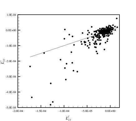
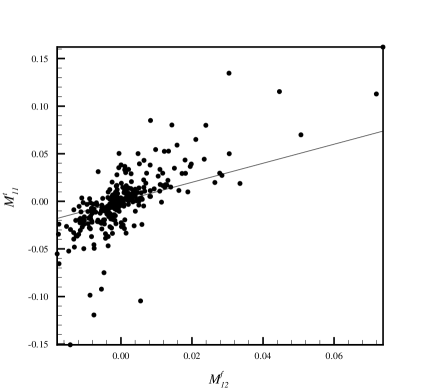
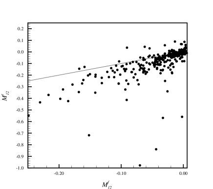
Figure 6: Scatter plots of the $L_{11}$, $L_{12}$, $M_{11}$, $M_{12}$ components in the $x-z$ plane at $y^{+}=43$ from filtered DNS of channel flow, comparing local values obtained from the derivative-based approach with the classical filter-based values.

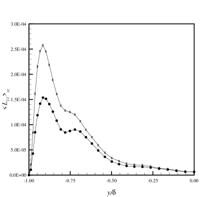
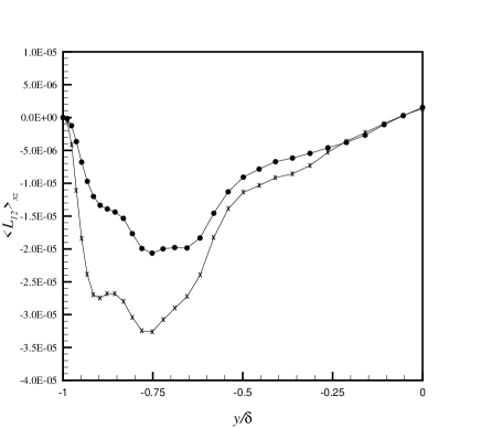
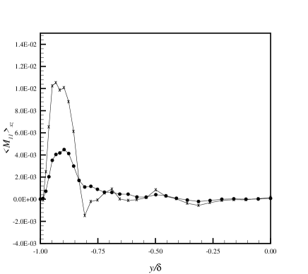
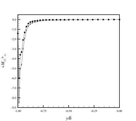
Figure 7: Comparisons of the mean components $L_{11}$, $L_{12}$, $M_{11}$, $M_{12}$ averaged in the $x$-$z$ planes across the wall normal direction. $\times$ derivative-based method, $\bullet$ classical filter-based method.

As a first step we perform a priori tests at the initial time of the LES simulations, which are filtered DNS fields. Scatter plots comparing the $L_{11}$, $L_{12}$, $M_{11}$, $M_{12}$ components obtained by the Taylor series and filtering based methods, in the $x$-$z$ plane at $y^{+}=43$, are shown in Figure 6. The agreement between real filtered and estimated local values is fair. The general trends are reproduced with correlation coefficients of order 0.7. Specifically $\rho(L^{t}_{11},L^{f}_{11})=0.79$, $\rho(L^{t}_{12},L^{f}_{12})=0.81$, $\rho(M^{t}_{11},M^{f}_{11})=0.74$, and $\rho(M^{t}_{12},L^{f}_{12})=0.64$. Even if the local behavior of the typical components of $L_{ij}$ and $M_{ij}$ is not highly accurate, the global behavior of these components is estimated reasonably well, as demonstrated by Figure 7, showing the same tensor elements averaged in the $x$-$z$ planes, as a function of wall normal direction. We notice that despite an overestimation of the magnitude of each component, their general shape is correctly predicted by the derivative-based approximation.

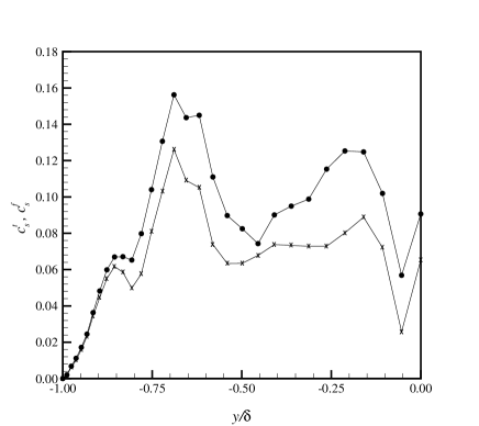
Figure 8: Dynamic Smagorinsky coefficients, obtained a priori from filtered DNS of minimal channel flow. $\times$ derivative-based method, $\bullet$ classical filter-based method.

Figure 8 shows the instantaneous Smagorinsky coefficients obtained by the classical filtering procedure and by the present derivative-based method. The a priori test shows that the Smagorinsky coefficient obtained by the Taylor series expansion approach is slightly smaller than the classical filter-based results. However, the agreement is sufficiently good in the context of a practical scheme, especially the reduction to zero in the well-resolved near-wall region. As we will see in the next section, a posteriori tests give improved results.

4.2.2 A posteriori results of LES

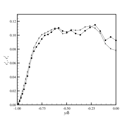
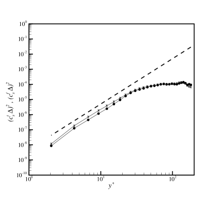
(a) (b)

Figure 9: Comparisons of the Smagorinsky coefficients obtained in a posteriori tests by the filter-based and derivative-based methods in the global (a) and wall (b) coordinates. Same symbols as in Figure 8. Dashed line is the expected $c_{s}^{2}\Delta^{2}\sim(y^{+})^{3}$ behavior.

All the results presented in this section are time-averaged over 55 realizations spaced by a time interval of $0.1\delta/u_{\tau}$. In Figure 9(a), we observe that the Smagorinsky coefficient is very well predicted by the derivative-based method, except some deviation near the centerline. As shown in Figure 9(b) the derivative-based approach yields the expected $y^{+3}$ behavior in the vicinity of the wall.

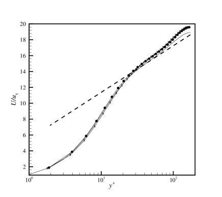
Figure 10: Mean Velocity U in wall coordinates: $-$ DNS, $\times$ derivative-based method, $\bullet$ classical filter-based dynamic model. Dashed line: $U/u_{\tau}=2.5\ln(y^{+})+5.5$.

In Figure 10, we observe a fairly good agreement in streamwise mean velocity $U$ between the results of the Taylor series expansion method and both the results of the classical filter-based dynamic model and the DNS results. Despite a slight underestimation in the buffer region, the proposed approach leads to quite accurate results.

In Figure 11 are shown the rms intensities of the large-scale (resolved) turbulent velocity fluctuations. These rms quantities are compared with the rms velocities from the DNS filtered at scale $\Delta$ using a box filter. The agreement between both LES results and the filtered DNS data is quite good. For the derivative based method, the streamwise rms velocity is slightly overestimated by both LES approaches. The wall-normal and transverse rms velocities are underestimated slightly more by the derivative-based method than the filter-based method. In Figure 11(d), we compare the Reynolds shear stress of the resolved velocity, $\langle\widetilde{u}^{\prime}\widetilde{v}^{\prime}\rangle$. The proposed approach yields very good agreement with the filter-based dynamic model and the reference filtered DNS data.

5 Conclusions

An implementation of the dynamic Smagorinsky model that uses Taylor series expansions to avoid explicit test-filter operations in LES has been developed. The proposed method has been subjected to a priori and a posteriori tests. These tests were performed using structured grids, to check the performance of the method in idealized, well controlled reference cases.

The a priori results obtained by truncating the Taylor series at $2^{\mathrm{nd}}$ order and at $4^{\mathrm{th}}$ order have been compared with results obtained by test filtering. It was found that for LES of isotropic turbulence, it is possible to obtain values of $c_{s}^{2}$ accurate to $\sim 5$ % by using the $2^{\mathrm{nd}}$ order approximation. However, results are not improved by using the $4^{\mathrm{th}}$ order approximation because of the errors associated with evaluating high-order derivatives on inherently rough LES fields. From these a priori tests, it is concluded that the derivative based method should be implemented using the $2^{\mathrm{nd}}$ order approximations, with $\alpha=2$. A posteriori tests of forced isotropic turbulence show that the derivative-based method yields stable results, and values of $c_{s}^{2}$ to within $\sim 10\%$ of those obtained by explicit test filtering.

Applications to a minimal channel configuration show that the observed differences between the tensor elements in the filter-based and Taylor series based approaches are larger than those in isotropic turbulence. This could be due to the strong anisotropy of the test filter as well as of the turbulence itself. However the Smagorinsky coefficient is correctly estimated by the proposed approach, especially the $y^{+3}$ behavior in the vicinity of the wall. Moreover first and second order statistics, which are the most important ones for practical engineering calculations, are correctly predicted when using the derivative-based dynamic model.

Strictly speaking, these conclusions are applicable only to the fairly simple flow configurations considered in this work. However, the results suggest that applications of the Taylor series based dynamic model to complex-geometry flows on unstructured grids is a promising direction. Taken together with the results of Jansen (1999) on the alternative generalized box-filter approach, the present results show that applications of the dynamic model to LES of complex-geometry turbulent flows are feasible.

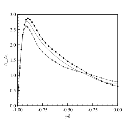
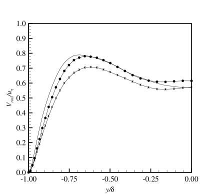
(a) (b)

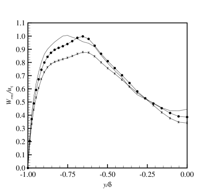
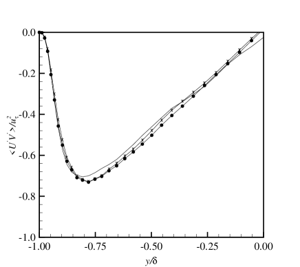
(c) (d)

Figure 11: (a)-(c) Comparisons between rms velocities from LES and filtered DNS velocity rms. (d) Comparison between Reynolds shear stresses $\langle\widetilde{u}^{\prime}\widetilde{v}^{\prime}\rangle$ from LES and filtered DNS. Same symbols as in Figure 10.

Table 1: Correlation coefficients, normalized square error, values of $c_{s}^{2}$, and relative error in $c_{s}^{2}$ obtained from a priori tests in forced isotropic turbulence.

$\alpha$	2						3	4
prefiltering	none				$4\Delta$		none
order of finite differences ($D=$ )	2		4		4		2
order of expansion ($T=$ )	2	4	2	4	2	4	2
$\rho({L}^{f}_{11},{L}^{t}_{11})$	0.955	0.978	0.946	0.981	0.993	1.000	0.889	0.791
$\rho({L}^{f}_{12},{L}^{t}_{12})$	0.947	0.976	0.932	0.977	0.993	1.000	0.863	0.748
$\rho({M}^{f}_{11},{M}^{t}_{11})$	0.996	0.990	0.995	0.986	1.000	1.000	0.832	0.380
$\rho({M}^{f}_{12},{M}^{t}_{12})$	0.998	0.993	0.996	0.989	1.000	1.000	0.868	0.415
$\mathcal{E}({L}^{f}_{11},{L}^{t}_{11})$	0.056	0.070	0.187	0.029	0.023	5.78E-4	0.369	1.301
$\mathcal{E}({L}^{f}_{12},{L}^{t}_{12})$	0.158	0.078	0.514	0.050	0.048	9.13E-4	1.264	4.556
$\mathcal{E}({M}^{f}_{11},{M}^{t}_{11})$	0.009	0.031	0.014	0.047	1.08E-4	3.03E-4	0.363	10.315
$\mathcal{E}({M}^{f}_{12},{M}^{t}_{12})$	0.006	0.025	0.009	0.040	1.02E-4	4.51E-4	0.268	7.845
$(c_{s}^{f})^{2}$	0.0151	0.0151	0.0126	0.0126	0.0097	0.0097	0.0156	0.0164
$(c_{s}^{t})^{2}$	0.0159	0.0110	0.0173	0.0104	0.0110	0.0094	0.0146	0.0005
error in $(c_{s}^{t})^{2}$ (%)	5.30	27.2	37.3	17.5	13.4	3.1	6.41	97.0