1 Introduction

In view of the completion of the first experimental phase at the Gran Sasso underground laboratory, new detector requirements are emerging, in the framework of possible activities with atmospheric neutrino detectors, long baseline neutrino beam from CERN[1] (CNGS), or (at present in a more speculative way) at neutrino factories. In all the cases, although for different reasons, muon spectrometers, identifying muon charge, and possibly to provide some momentum reconstruction[2, 3] are required. The small neutrino cross section reflects in large area and/or volume experiments: it is therefore mandatory to rely upon detector choices which can assure reasonable accuracies on the basis of a well assessed technology, reducing as much as possible the number of electronic channels to be implemented. The experience acquired with the already existing underground detectors suggests possible solutions. For example, streamer tube chambers[4] with a cell size of about 3x3 $cm^{2}$, similar to those developed for the MACRO experiment[5], could be operated as drift tubes. These devices were originally operated in digital mode, with wire and pick up strip readout in two coordinates, for the recognition of charged track pattern, with a point resolution of about 1 cm. Therefore they have been operated with simple electronics and without stringent stability and uniformity monitoring. Furthermore, these devices have been exhibiting a remarkable reliability, being capable of continuous operation for more than ten years.

The space resolution required by a massive muon spectrometer analyzing muons from neutrino interaction in a Long Base line experiment is limited by the multiple scattering occurring in the magnetized iron: a space resolution of $\sim$ 1mm is considered satisfactory. Similar considerations apply to the case of atmospheric neutrino detectors. For this reason it is worthwhile to investigate the attainable space resolution of these devices. It is already known in literature how the streamer regime can be advantageous for drift operation, provided that a low rate environment exists[6]: in that paper the results obtained using a streamer tube cell with cross section (0.9x0.9) $cm^{2}$ were reported, showing a resolution $\sigma_{x}$$\simeq$150$\mu$m. The goal of this paper is to show that large size cell streamer tubes, constructed in the “coverless” field configuration[4], even if their electric field cannot be considered as optimal and even if the accuracy in their mechanical construction is not better than 0.1 mm, can achieve the required space resolution.

According to the present safety rules, it is not conceivable to reconvert the already existing tubes of MACRO since they are built in PVC. However, they can be constructed with a different, non dangerous, thermo–plastic material, for instance ABS(Acrylonitrile-Butadiene-Styrene), always ensuring fabrication costs which are advantageous with respect to other wire-device solutions.

To measure the resolution attainable in drift mode with a streamer tube device with large cells, we made a specific test on an 8-wire “coverless tube” chamber of the same kind as used in the MACRO experiment, with the only difference of being 50 cm long. The test has been performed selecting cosmic ray tracks by means of a high precision telescope realized with silicon pixel arrays. After the description of the test set-up, we shall describe the calibration of the measurement and the experimental results.

2 Set up description

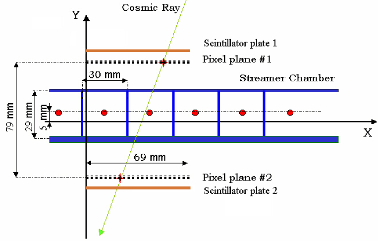
Figure 1: Sketch of the setup used for the measurement.

The experimental setup for the test consisted of a high precision cosmic ray telescope and the streamer chamber under test (Fig.1). The telescope was built using two planes of silicon pixel arrays and two plastic scintillators (20x70x10) mm³ for triggering purposes. The silicon pixel detectors used were arrays of 8064 pixels with dimensions of (330 x 330) $\mu$m², and a thickness of about 300$\mu$m. These pixels are readout in digital mode, providing thus only the coordinates of the pixels hit by a particle. These detectors are the same as the ones used in the DELPHI Very Forward Tracker (VFT, [7, 8]). The active area of 990 mm² is divided into 10 regions of 24x24 pixels, followed by six regions of 24x16 pixels, for a total length of 69mm and a width of 22mm and 17mm respectively. Typical figure of merit of these detectors are $\epsilon\approx~{}99\%$, with a threshold around 10,000 electrons, a number of noisy pixels at 0.3% level and a point resolution of 100$\mu$m in both coordinates.

A 50 cm long chamber of the same kind of those used in MACRO has been positioned in the middle plane of the telescope (Fig. 1). The description of the plastic streamer tubes of MACRO has been extensively reported in [5] and references therein. We remind here that the basic unit of the tube system is a chamber containing eight individual cells. The single cell is (2.9 x 2.7) cm². The anode wire (silvered Be-Cu) has a diameter of 100 $\mu$m. Three sides of the cell are coated with a low–resistivity graphite ($<1~{}k\Omega$/square) to perform the cathode function by the electrode-less shaping principle [10]. This structure is inserted inside an uncoated PVC envelope (1.5 mm thick) and closed by two plastic end caps at the ends. The overall external size of our chamber is 3.2 cm x 25 cm x 50 cm. Each wire behaves as a transmission line with a characteristic impedance of 330 $\Omega$ and a propagation time sligthly larger than 3.3 ns/m. They provide both digital readout for tracking and analog (charge) readout. The chamber is fluxed with an Argon + Isobutane with relative fractions of 50/50 gas mixture, controlled within a 15% accuracy. In these operation conditions, full efficiency is achieved for an anode high voltage value of about 5500 V, with a single counting rate plateau spanning from 5200 V to 5900 V. The operation properties of streamer tubes operating with various gas mixtures has been extensively studied in [4, 5, 11] and references therein. The field configuration of the coverless MACRO tube cell can be derived from Fig. 2 which shows the equipotential lines as obtained with the GARFIELD program[12] for an anode voltage of 5500 V.

The geometry of the setup is sketched in Fig. 1. A cartesian coordinate system is defined , having the x axis parallel to the long side of the pixel detectors, the z axis parallel to the short side of the pixel detectors and to the wires of streamer tube. As a consequence the y axis is perpendicular to the plane of the detectors. Since the pixel detectors are only 69 mm long, the trigger area covers 2 cells and the edge region of the adjacent ones. All the measurements reported here have been performed with a distance between the silicon planes of 79 mm. In this configuration, we triggered only tracks with an angle with respect to the vertical not exceeding 35^∘, with a most probable value around $10^{\circ}$. The cosmic trigger rate was of $\sim$1 track/min.

The accuracy in the determination of the track position at the wire level, taking into account the multiple scattering in the silicon pixels and in the streamer tube walls, is $<$90 $\mu$m, assuming an average muon energy of $\sim$1 GeV. The trigger signal is provided by the coincidence of the scintillator pulses. The telescope is readout by means of a Pixel Readout Repeater, driven by a Pixel Camac Board[7], that provides the necessary timing signals and the power supply lines. The signal from the tube wires are OR-ed together by means of a resistive network, providing an output signal on 50 $\Omega$ impedance. The wire pulses are properly discriminated ($50mV/50\Omega$) and sent to a TDC (Lecroy 2228A), which records the time difference between the scintillator trigger signal and the streamer chamber signals. The TDC was used with a 1bit resolution of 250ps.

The acquisition chain has been realized by means of a Labview application, developed in our group, and was controlled by a PC equipped with a GPIB CAMAC controller (Lecroy 8901 A). The acquisition included also a scaler (Lecroy 2551) to record the counts of the scintillators and of the singles tubes, in order to perform stability checks. The Pixel Readout runs continuously a gate–reset sequence until a scintillator trigger in coincidence with the gate is received. In this case the first bit of an input/output register is used to control the synchronization between the PC and the Pixel Camac Board. The acquisition monitoring is provided by a graphical interface.

3 Detector calibration

As a first step, we used a small data sample to have a precise geometrical survey of the actual position of the wires. Fig. 3 shows the drift distance as a function of the X position computed at the wires level Y=0, measured by using the silicon pixel detector. The wires are of course positioned where the drift distance reaches his minimum, i.e. at the lower cusp points of the v–shaped distributions. By means of a linear fit to the four straight portions of this scatter plot we obtained $X_{wire~{}1}$ =(1.95$\pm$0.05)cm and $X_{wire~{}2}$  =(4.85$\pm$0.05)cm. A first measurement of the average drift velocity $V_{drift}$ (neglecting differences as a function of the distance from the wire) can be obtained by selecting vertical tracks and imposing:

$$Max(TDC)\cdot R_{TDC}\cdot V_{drift}=Cell/2,$$ (1)

where Max(TDC) is the maximum value of the TDC in the data sample, $R_{TDC}$ is the conversion factor from TDC channels to ns and Cell/2 is half of the cell length. The actual cell width of each tube is known with an accuracy of 0.1 mm.

The value of $R_{TDC}$ has been calibrated to be $R_{TDC}$=0.242ns/channel and $R_{TDC}$=0.248ns/channel for the first and the second cell respectively. The resulting average drift velocity from the above mentioned data sample was found to be $V_{drift}$=(4.5 $\pm$ 0.3) cm/$\mu$s.

Data were collected at different operation high voltage, ranging from 5500 V to 5900 V, by using simultaneously two tube cells. The gas mixture was kept unchanged.

We do not expect a constant drift velocity as a function of position. Therefore, in order to derive a more accurate estimate of the space-time relation, we adopted the following method for each different set of operation conditions.

We have computed the minimum track-wire distance in two ways:

1. $D_{drift}$, using the drift time measurement (according the average drift velocity quoted above);

2. $D_{Si}$, using the track reconstructed from pixel readout.

If we plot $D_{drift}$ versus $D_{Si}$ as in the top panel of Fig. 4, a clear deviation from linearity is observed. We made the assumption that the required correction depends only on the cell geometry, the gas mixture and the high voltage, being independent of the specific cell used. Under this hypothesis we considered together the data from the two cells and a correction as a a function of $D_{Si}$ was introduced to restore linearity. Such correction is achieved by fitting the scatter plot with a piece-wise linear fit, so that 2 parameters for each $D_{Si}$ section are obtained from the law:

$$L(cm)=p_{0}+p_{1}\cdot TDC\cdot R_{TDC}\cdot V_{drift}$$ (2)

The $p_{0}$ and $p_{1}$ values are reported in Table 1.

Distance from wire (cm)	$p_{O}$ (cm)	$p_{1}$
0. – 0.65	-0.014	1.13
0.65 – 1.0	0.266	1.02
1.0 – 1.5	0.016	0.95

Table 1: Values of fitted parameters in the correction algorithm for the three different distance regions at the 5500 V operation point.

The bottom panel of Fig. 4 shows the distribution of data after correction. Such procedure can be applied to any streamer tube cell working in an actual experiment.

4 Experimental results

The overall space accuracy from the drift time measurement can be obtained from the distribution of the residuals of the fit of Fig. 4 (bottom panel), summing up all cells.

The results are shown in Fig. 5 for HV = 5500 V and 5900 V. The gaussian fits give a resolution of $\sigma_{tot}$=(271$\pm$7)$\mu$m and $\sigma_{tot}$=(207$\pm$5)$\mu$m for HV = 5500, 5900 V respectively. The standard deviation of such distributions can be written as $\sigma_{tot}$= $\sqrt{\sigma_{drift}^{2}+\sigma_{Si}^{2}}$= 271 $\mu$m (207 $\mu$m). Since the silicon pixel size is 330 $\mu$m the ideal contribution of $\sigma_{Si}$ to $\sigma_{tot}$ would be $\sigma_{Si}$=330 $\mu$m/$\sqrt{12}$/$\sqrt{2}$=68 $\mu$m and hence the intrinsic space resolution achievable with the drift time method would be $\sigma_{drift}$= $\sqrt{\sigma_{tot}^{2}-\sigma_{Si}^{2}}$=262 $\mu$m (195 $\mu$m). Taking into account also the expected muon momentum distribution ($<E_{\mu}>\sim$ 1 GeV) and the multiple scattering inside the silicon and the chamber walls, we obtain an average value of $\sigma_{Si}$=94. The estimated value of $\sigma_{drift}$ then improves and it is $\sigma_{drift}$=254 $\mu$m (184 $\mu$m).

We also tried to measure $\sigma_{drift}$ as a function of the X distance from the wire, selecting different track samples on the basis of the track parameters reconstructed with the silicon detector. In order to maintain an high efficiency and reliability of the streamer tubes system in large area detectors, the HV has to be kept within the plateau, so we did not attempt to go beyond HV=5900 V. The results are shown in Fig. 6. We can identify at 5900 V an optimal $\sigma_{drift}$ in the central part of the tube, i.e. X$\simeq$ 0.7 cm. At lower X, the resolution is spoiled by a probable non linear space–time relation, while at large X it is affected by the reduced electrical field in proximity of the cell walls and corners. The resolution improves increasing the HV, due to the reinforcement of the electric field in the cell wall neighbourhood.

In order to verify these hypotheses, we simulated the expected drift velocity as a function of distance from the wire using the GARFIELD package. To take into account the trigger acceptance, we used an angular distribution taken from real data tracks, reconstructed with the silicon pixel detector. The (x,y) position corresponding to the minimal distance from the wire was estimated for each track and used as input to the GARFIELD simulation. The curve in Fig.7 shows the simulated drift velocity as a function of the distance from the wire, for HV=5500 V. The simulation is obtained changing the Isobutane fraction in the gas mixture from 40$\%$ to 60 $\%$. An higher fraction of quenching gas reflects in a smaller drift velocity at low electric field (i.e. near the tube walls). The experimental data are in satisfactory agreement with the GARFIELD simulation. The space resolution quoted above could be in principle slightly spoiled in a longer streamer cell, due to the wire sagitta.

5 Discussion and conclusions

The performance of a large streamer tube cell in drift mode have been tested using an high precision silicon telescope: space resolution between 150 $\mu$m and 350 $\mu$m have been obtained, depending on the HV applied and on the track distance from the wire.

Such quite good resolution, can be anyway spoiled, when using streamer tubes in drift mode for real spectrometers:
a) In case of longer tubes, the practically achievable resolution is deteriorated by the wire sag position determination. This problem is always present in any long tube: the relevance of such effects depends on the geometry of the tube. Should the magnetic field deflection lye in the same plane where the gravitational force applies, the resolution deterioration would be more severe.
b) Concerning non superconducting spectrometer, equipped with iron, the space resolution is deteriorated by $\delta$-rays and electrons-positrons pairs produced in the magnetic field iron yoke, penetrating inside the cell. When a muon crosses the cell close to the walls, such particles may result in earlier streamer avalanches, producing thus shorter drift times.
c) As it has been pointed out in [6], inclined tracks may hit streamer tube cells at different coordinates along the wires, introducing thus additional delays. Due to the relatively fast signal velocity transmission along the wire, $\simeq$25 cm/ns, compared to standard drift velocity, a rough knowledge of the coordinate of the event along the wire, ($\simeq$ 1m) is required to recover the full resolution.

Summarizing, although realistic spectrometers equipped with streamer tubes operating in drift mode, may suffer the space resolution deterioration quoted above, the expected resolution is anyway well below 1 mm. Taking into the account the multiple scattering suffered by muons in the iron, such resolution is still adequate to fulfill the requirements for massive iron spectrometers for neutrino physics, indicating streamer tubes in drift mode as a possible choice for particle tracking in muon charge and momentum analysis.

Figure 2: Equipotential line in the streamer tube cell operating at the 5500 V anode voltage.

Figure 3: Track distance from the wire, as reconstructed with the time measurement, as a function of the position in the cell as reconstructed from the pixel telescope.

Figure 4: Distance from the wire as obtained from the drift measurement vs the distances obtained from the pixel telescope. Upper panel: results using a drift velocity averaged on the cell width. Lower panel: after corrections applied to take into account the variation of drift velocity as a function of the distance from the wire. The straight line is put to guide the eye.

Figure 5: Distribution of the difference between the track position obtained from the drift measurement and from the position detector.

Figure 6: Position resolution achieved with the streamer tube in drift mode as a function of the coordinate along the wire plane, for three different operation voltages.

Figure 7: Comparison of the expected drift velocity (GARFIELD) with the present results.

References

- [1] CERN 98-02 – INFN/AE 98-05; CERN/SL 99-04(DI) – INFN/AE 99-05.
- [2] CERN/SPSC 98-25; SPSC/M612LNGS-LOI 8/97 Original Letter of Intent (1997); CERN/SPSC 98-25, LNGS-LOI 8/97, Addendum to the Letter of Intent (1998); CERN/SPSC 99-20, SPSC/M635, LNGS-LOI 19/99 Progress Report; CERN/SPSC 99-38, SPSC/M641, LNGS-LOI 19/99 Add.1
- [3] LNGS-P21/99 – INFN/AE-99-17; CERN/SPSC 99-25 – SPSC/P314.
- [4] G. Battistoni, Nucl Instr. & Meth A279 (1989) 137.
- [5] Ahlen et al., Nucl. Instr. & Meth. A234 (1993) 337.
- [6] F. Gasparini et al., Nucl. Instr. & Meth A267 (1988) 87.
- [7] P. Chochula et al., Nucl. Instr. & Meth A412 (1998) 304.
- [8] K.H. Becks et al., Nucl. Instr. & Meth A386 (1997) 398.
- [9] M. Solal, J.C. Clemens, Nucl. Instr. & Meth A380 (1996) 335.
- [10] G. Battistoni et al., Nucl. Instr. & Meth. 217 (1983) 429; J. Allison et al., Nucl. Instr. & Meth. 201 (1982) 341; C. Becker et al., Siegen University preprint SI-82-1 (1982).
- [11] G. Battistoni et al., Nucl. Instr. & Meth. 235 (1985) 91; G. Battistoni et al., Il Nuovo Cimento, Vol. 9C N.2 (1986) 653.
- [12] R. Veenhof, Nucl. Instr. & Meth. A419 1998, 726.