On the interaction of point charges
in an arbitrary domain

Abstract

We develop a systematic approach to calculating the electrostatic force between point charges in an arbitrary geometry with arbitrary boundary conditions. When the boundary is present, the simple expression for the force acting on a charge as “the charge times the field it is placed in” becomes ill-defined. However, this rule can be salvaged if the field in question is redefined to include all the terms that do not diverge at the charge position, in particular, those due to the charge itself. The proof requires handling the self-action energy divergence for point charges, which is accomplished by means of a geometrical regularization.

I Introduction

It is trivial to determine the force exerted by an external field on a point charge in an otherwise empty space: by definition, “the force is equal to the charge times the field it is placed in”. In particular, if the field in question is created by some other point charges, this rule, known by many from high school, still holds.

However, the situation changes drastically when a set of point charges creates the field inside an arbitrary domain with a boundary of some physical origin (reflected in the appropriate boundary conditions). Now the very notion of “the field the charge is placed in” becomes not well defined. For example, a naive treatment of a single–charge problem might lead one to an entirely wrong conclusion that, since all the field in the problem is due to the charge itself (there are no other sources!), “the field it is placed in” is zero, so there is no force at all.

A slightly more sophisticated physicist would argue that only the part of the field which diverges as $1/r^{2}$ near the charge is really created by it, while the rest is due to the boundary conditions, which represent mathematically the rearrangement of other physical charges at the boundary. Therefore it is precisely what remains after subtracting the singular part that now gives “the field the charge is placed in”. Unfortunately, such treatment leaves one in a somewhat awkward position of, first, calculating potentials and fields rigorously, and then lowering the plank and using hand-waving arguments to derive forces from them. It is also not clear whether the guess about which part of the total field contributes to the force is always valid.

Thus it seems appealing to show that the physical arguments can be backed by an accurate mathematical proof demonstrating that the adjusted rule, “the force is equal to the charge times the part of the field that does not diverge at the charge’s location”, is either universal or limited by certain conditions. To do this, one should turn to the most fundamental energy conservation argument which gives the force as the negative gradient of the energy in the charge’s position. This approach also does not turn out to be straightforward, since the energy is infinite in the presence of point charges due to their self–action.

Perhaps because of these difficulties, as well as of a misleading apparent simplicity of the problem, our literature search, which encompassed, in particular, Refs. zomm, ; tamm, ; strat, ; llf, ; llc, ; smy, ; jack, ; feynman, ; cro, ; moo, and many other books on the subject, revealed no ready result (except for one small piece in Ref. smy, which we discuss in Sec. IV). So we give a careful derivation of the general expression for the force on point charges in this paper. It consists of a regularization of the problem, calculation of the force from the (regularized and finite) energy, and then taking the singular limit. The result agrees with one’s intuitive expectations.

II Electrostatics problem with volume point charges: potential and energy

Consider an arbitrary 3-dimensional domain $D$ with the perfectly conducting boundary $S$ and some $N$ point electrical charges inside. The electrical potential, $\psi({\bf r})$, in this case is determined by the following Dirichlet boundary value problem (we use SI units throughout the paper):

$$\Delta\psi = -\frac{1}{\varepsilon_{0}}\sum_{i=1}^{N}q_{i}\,\delta\left({\bf r}-{\bf r}_{i}\right),\quad{\bf r},\,\,{\bf r}_{i}\in D;$$ (1)

$$\psi\,\biggl{|}_{S} = 0\,.$$ (2)

Here ${\bf r}=x{\bf e}_{x}+y{\bf e}_{y}+z{\bf e}_{z}$ is the vector radius of a point, and ${\bf r}_{i}=x_{i}{\bf e}_{x}+y_{i}{\bf e}_{y}+z_{i}{\bf e}_{z}$ specifies the $i$th charge position, with ${\bf e}_{\alpha},\,\,\alpha=x,y,z$, being the unit vectors in the direction of the corresponding Cartesian axes.

By superposition principle, the potential $\psi({\bf r})$ is just the sum of the potentials induced by each charge separately,

$$\psi({\bf r}) = \kappa\sum_{j=1}^{N}q_{j}G({\bf r},{\bf r}_{j})$$ (3)

$$\equiv \kappa\sum_{j=1}^{N}q_{j}\left[\frac{1}{|{\bf r}-{\bf r}_{j}|}+G_{R}({\bf r},{\bf r}_{j})\right],$$ (4)

where $\kappa=1/4\pi\varepsilon_{0}$, and $G_{R}({\bf r},{\bf r}_{j})$ is the regular part of the Green’s function $G({\bf r},{\bf r}_{j})$ of the corresponding boundary value problem [set $q_{j}=1,\,\,q_{i}=0,\,\,i\not=j$ in Eq. (1)]. Both functions are, of course, symmetric in their arguments,

$$G({\bf r},{\bf r}_{j})=G({\bf r}_{j},{\bf r}),\qquad G_{R}({\bf r},{\bf r}_{j})=G_{R}({\bf r}_{j},{\bf r}).$$ (5)

Furthermore, we can rewrite Eq. (4) splitting the potential in a sum of its singular and regular parts,

$$\psi({\bf r}) = \kappa\sum_{j=1}^{N}\frac{q_{j}}{|{\bf r}-{\bf r}_{j}|}+\psi_{R}({\bf r}),\quad$$ (6)

$$\psi_{R}({\bf r}) \equiv \kappa\sum_{j=1}^{N}q_{j}G_{R}({\bf r},{\bf r}_{j})\;,$$ (7)

where $\psi_{R}({\bf r})$ is a regular function satisfying the Laplace equation everywhere in $D$ [by continuity, this holds also at any regular point of the boundary $S$, although this is irrelevant to our discussion]. Note that both the potential, $\psi$, and its regular part, $\psi_{R}$, depend actually on the positions of the charges ${\bf r}_{i}$ as well as on the observation point ${\bf r}$, which is reflected in the full notation,

$$\psi({\bf r}) \equiv \psi({\bf r},\,{\bf r}_{1},\dots,{\bf r}_{i},\dots,{\bf r}_{N}),\quad$$ (8)

$$\psi_{R}({\bf r}) \equiv \psi_{R}({\bf r},\,{\bf r}_{1},\dots,{\bf r}_{i},\dots,{\bf r}_{N}).$$ (9)

We assume that the potential is known and are interested in finding the force ${\bf F}^{i}$ acting on the charge $q_{i}$. From the energy conservation for the considered problem, the force is given by (cf. Ref. smy, )

$${\bf F}^{i}=-\frac{\partial}{\partial{\bf r_{i}}}W_{D}\,,\;\;\;\frac{\partial}{\partial{\bf r_{i}}}=\frac{\partial}{\partial x_{i}}{\bf e}_{x}+\frac{\partial}{\partial y_{i}}{\bf e}_{y}+\frac{\partial}{\partial z_{i}}{\bf e}_{z}\;,$$ (10)

where $W_{D}$ is the energy of the field in the volume $D$,

$$W_{D}=\frac{\varepsilon_{0}}{2}\,\int_{D}(\mbox{\boldmath$\nabla$}\psi)^{2}\,dV.$$ (11)

Note that we alternatively write $\nabla$ or $\partial/\partial{\bf r}$ for the gradient, whatever seems proper in a particular expression.

The problem is, however, that the above integral obviously diverges due to self-interaction of the point charges (the energy of a single point charge is infinite). We are going to show that even though the energy for a given point charge distribution is infinite, the difference between its two values corresponding to two different but close charge configurations is finite for any charge configuration and boundary shape, and the force is also finite due to that, in accordance with common intuition.

III Regularized energy and the force on the charges

We surround each volume charge $q_{i}$ by a small sphere $S_{i}^{\epsilon}$ of radius $\epsilon$; we write $D_{i}^{\epsilon}$ for the ball inside it. We define $D^{\epsilon}$ as $D$ without all domains $D_{i}^{\epsilon}$, and $S^{\epsilon}$ as a union of ${S}$ and all spherical surfaces $S_{i}^{\epsilon}$ (see Fig. 1). In effect, $S^{\epsilon}$ is the boundary of $D^{\epsilon}$.

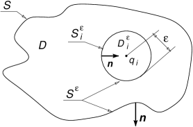
Figure 1: Volumes, surfaces, and normal directions involved.

Using Eq. (10), we may now define the force acting on the charge $q_{i}$ as

$${\bf F}^{i}=\lim_{\epsilon\to 0}{\bf F}^{i}_{\epsilon}=-\lim_{\epsilon\to 0}\frac{\partial}{\partial{\bf r_{i}}}W_{D}^{\epsilon},$$ (12)

where $W_{D}^{\epsilon}$ is the regularized energy, that is, the energy of the field in $D^{\epsilon}$, which is finite. It is important to note the order of operations in Eq. (12): first take the gradient of the regularized energy in the charge position, then take the (singular) limit. In principle, we also have to show that the final result does not depend on the regularization chosen, but this task is not easy. We will return to it briefly later in this paper.

In view of Eq. (11) and the fact that the total potential given by Eq. (3) or Eq. (6) is regular in $D^{\epsilon}$, the regularized energy is

$$W_{D}^{\epsilon} \equiv \,\frac{\varepsilon_{0}}{2}\int_{D^{\epsilon}}(\mbox{\boldmath$\nabla$}\psi)^{2}\,dV$$ (13)

$$= \frac{\varepsilon_{0}}{2}\int_{S^{\epsilon}}\psi\frac{\partial\psi}{\partial{n}}\,d{A}-\frac{\varepsilon_{0}}{2}\int_{D^{\epsilon}}\psi\Delta\psi\,dV;$$ (14)

$n$ is the direction of the outward normal to $S^{\epsilon}$ (and thus the inward normal to the spheres $S_{i}^{\epsilon}$). For an infinite domain $D$ it is assumed here that the potential and its gradient drop at infinity fast enough to make the contribution of integrating over the sphere of a large radius vanishing in the limit, which assumption has to be verified in each particular case.

Since $\psi$ is harmonic everywhere in $D^{\epsilon}$, the volume integral on the right of the previous equality vanishes; the remaining surface one is represented as

$$W_{D}^{\epsilon}=\frac{\varepsilon_{0}}{2}\sum_{k=1}^{N}\int_{S_{k}^{\epsilon}}\psi\frac{\partial\psi}{\partial{n}}\,d{A}+\frac{\varepsilon_{0}}{2}\int_{S}\psi\frac{\partial\psi}{\partial{n}}\,d{A}$$ (15)

and then, because of the boundary condition, Eq. (2), as

$$W_{D}^{\epsilon}=\frac{\varepsilon_{0}}{2}\sum_{k=1}^{N}\int_{S_{k}^{\epsilon}}\psi\frac{\partial\psi}{\partial{n}}\,d{A}.$$ (16)

We are ultimately interested in the limit $\epsilon\to 0$, so we need to calculate only the quantities which do not vanish in this limit. The area of integration in each term of the above sum is $O(\epsilon^{2})$, therefore we need to keep track of the integrands that grow at least quadratically in $\epsilon^{-1}$. Bearing this in mind and using Eq. (6) for the potential, we can write the surface integral in Eq. (16) as

$$\int_{S_{k}^{\epsilon}}\psi\frac{\partial\psi}{\partial{n}}\,d{A}=\int_{S_{k}^{\epsilon}}\frac{\kappa\,q_{k}}{|{\bf r}-{\bf r}_{k}|}\,\frac{\partial}{\partial{n}}\left(\frac{\kappa\,q_{k}}{|{\bf r}-{\bf r}_{k}|}\right)\,d{A}+\int_{S_{k}^{\epsilon}}\left[\psi_{R}({\bf r})+\sum_{j=1,j\neq k}^{N}\frac{\kappa\,q_{j}}{|{\bf r}-{\bf r}_{j}|}\right]\,\frac{\partial}{\partial{n}}\left(\frac{\kappa\,q_{k}}{|{\bf r}-{\bf r}_{k}|}\right)\,d{A}+O(\epsilon)\;.$$ (17)

The first term in the above expression is, in fact, a regularized self–energy of the $k$-th charge, $W_{k,\,self}^{\epsilon}$. Doing an elementary integration, we immediately find that

$$W_{k,\,self}^{\epsilon}=\frac{\varepsilon_{0}}{2}\,\kappa^{2}\,\frac{4\pi q_{k}^{2}}{\epsilon}=\frac{\kappa\,q_{k}^{2}}{2\epsilon}\,.$$ (18)

The only feature of the regularized self–energy given by Eq. (18) important for our derivation is that it does not depend on the position of the charge $q_{k}$, i. e., on the vector radius ${\bf r}_{k}$.

The second term of the r. h. s. of Eq. (17) can also be simplified if one notices that both $\psi_{R}$ and $1/|{\bf r}-{\bf r}_{j}|$, $j\neq k$, are regular on $S_{k}^{\epsilon}$ and in $D_{k}^{\epsilon}$. Therefore their change within the small surface $S_{k}^{\epsilon}$ is of order $\epsilon$. Thus Eq. (17) may be rewritten as

$$\frac{\varepsilon_{0}}{2}\int_{S_{k}^{\epsilon}}\psi\frac{\partial\psi}{\partial{n}}\,d{A} = {W_{k,self}^{\epsilon}}+\frac{\varepsilon_{0}}{2}\left[\psi_{R}({\bf r_{k}})+\sum_{j=1,\,j\neq k}^{N}\frac{\kappa\,q_{j}}{|{\bf r}_{k}-{\bf r}_{j}|}\right]\int_{S_{k}^{\epsilon}}\frac{\partial}{\partial{n}}\left(\frac{\kappa\,q_{k}}{|{\bf r}-{\bf r}_{k}|}\right)\,d{A}+O(\epsilon)$$ (19)

$$= W_{k,self}^{\epsilon}+\frac{q_{k}}{2}\left[\psi_{R}({\bf r_{k}})+\sum_{j=1,\,j\neq k}^{N}\frac{\kappa\,q_{j}}{|{\bf r}_{k}-{\bf r}_{j}|}\right]+O(\epsilon),$$

and the integration here yielding the factor $4\pi$ is again an elementary one. This asymptotic equality may be differentiated in ${\bf r}_{i}$ with the same estimate of the remainder term.

Introducing now the last expression into the Eq. (16), we obtain:

$$W_{D}^{\epsilon} = \sum_{k=1}^{N}W_{k,\,self}^{\epsilon}\;+\;\frac{\kappa}{2}\sum_{k=1}^{N}\sum_{j=1,\,j\neq k}^{N}\frac{q_{j}\,q_{k}}{|{\bf r}_{j}-{\bf r}_{k}|}\;+\;\frac{1}{2}\sum_{k=1}^{N}q_{k}\psi_{R}({\bf r}_{k})\;+\;O(\epsilon)\;.$$ (20)

Equation (20), in its turn, is inserted in the Eq. (12) for the force; as shown, the self–energies do not depend on the charge positions, hence, although diverging in the limit $\epsilon\to 0$, they do not contribute to the force. The rest is pretty straightforward, except one has to be careful when differentiating the last term on the right of Eq. (20) with $k=i$: as seen from Eq. (8), in this case ${\bf r}_{i}$ stands for two (and not one!) arguments of $\psi_{R}$, namely, $\psi_{R}({\bf r_{i}})\equiv\psi_{R}({\bf r}_{i},{\bf r}_{1},\dots,{\bf r}_{i},\dots,{\bf r}_{N})$, and both of them have to be differentiated. Bearing this in mind, the expression for the force finally becomes:

$${\bf F}^{i} = -\kappa q_{i}\sum_{k=1,k\neq i}^{N}\frac{\partial}{\partial{\bf r_{i}}}\frac{q_{k}}{|{\bf r}_{i}-{\bf r}_{k}|}\;-\;\frac{1}{2}\left[\sum_{k=1}^{N}q_{k}\frac{\partial}{\partial{\bf r_{i}}}\psi_{R}({\bf r})\biggl{|}_{\bf r=\bf r_{k}}+q_{i}\frac{\partial}{\partial{\bf r}}\psi_{R}({\bf r})\biggl{|}_{{\bf r}={\bf r}_{i}}\right]$$ (21)

$$= \kappa q_{i}\sum_{k=1,k\neq i}^{N}q_{k}\frac{{\bf r}_{i}-{\bf r}_{k}}{|{\bf r}_{i}-{\bf r}_{k}|^{3}}\;-\;\frac{1}{2}\left[\sum_{k=1}^{N}q_{k}\frac{\partial}{\partial{\bf r_{i}}}\psi_{R}({\bf r})\biggl{|}_{\bf r=\bf r_{k}}+q_{i}\frac{\partial}{\partial{\bf r}}\psi_{R}({\bf r})\biggl{|}_{{\bf r}={\bf r}_{i}}\right]\;.$$

This is the general result for the electrostatics which can be transformed further in some nice way. Indeed, the direct substitution of the expression for $\psi_{R}$ from the Eq. (6) in the the Eq. (21) provides the force in the form

$${\bf F}^{i} = -\kappa q_{i}\sum_{k=1,k\neq i}^{N}\frac{\partial}{\partial{\bf r_{i}}}\frac{q_{k}}{|{\bf r}_{i}-{\bf r}_{k}|}\;-\;\frac{\kappa q_{i}}{2}\left[\sum_{k=1}^{N}q_{k}\frac{\partial}{\partial{\bf r_{i}}}G_{R}({\bf r},{\bf r}_{i})\biggl{|}_{\bf r=\bf r_{k}}+\sum_{j=1}^{N}q_{j}\frac{\partial}{\partial{\bf r}}G_{R}({\bf r},{\bf r}_{j})\biggl{|}_{{\bf r}={\bf r}_{i}}\right]$$ (22)

$$= -\kappa q_{i}\left[\sum_{k=1,k\neq i}^{N}\frac{\partial}{\partial{\bf r_{i}}}\frac{q_{k}}{|{\bf r}_{i}-{\bf r}_{k}|}\;+\;\sum_{k=1}^{N}q_{k}\frac{\partial}{\partial{\bf r}}G_{R}({\bf r},{\bf r}_{k})\biggl{|}_{{\bf r}={\bf r}_{i}}\right],$$

and we have used the symmetry property of Eq. (5) to obtain the second equality here. To make the result even more physically transparent, we rewrite Eq. (22), in its turn, in the following way:

$${\bf F}^{i}=-\kappa q_{i}\mbox{\boldmath$\nabla$}\left\{\sum_{k=1}^{N}q_{k}\left[\frac{1}{|{\bf r}-{\bf r}_{k}|}+G_{R}({\bf r},{\bf r}_{k})\right]-\frac{q_{i}}{|{\bf r}-{\bf r}_{i}|}\right\}\Biggl{|}_{{\bf r}={\bf r}_{i}}=-q_{i}\mbox{\boldmath$\nabla$}\left[\psi({\bf r})-\frac{\kappa\,q_{i}}{|{\bf r}-{\bf r}_{i}|}\right]\Biggl{|}_{{\bf r}={\bf r}_{i}}\;.$$ (23)

Note that the last expression, indeed, coincides with our intuitive guess for the form of the force.

IV Discussion

Our first remark on the expressions for the force in Eqs. (21)–(23) is that for the charges in a free space (volume $D$ is the whole space, no boundaries present) apparently $G_{R}({\bf r},{\bf r}_{k})\equiv 0,\,\psi_{R}\equiv 0$, and the classical Coulomb formula for the force is restored.

Next, Eq. (23) shows that the rule “the force is the charge times the field it is placed in” does work if one counts the regular part of the field produced by the charge in question as a part of the “field the charge is placed in”. It also makes up to some “minimal principle”, namely: to get the right answer for the force, one should throw out of the field only the part which otherwise makes the result infinite, and nothing beyond that. As we mentioned in the Introduction, this result is supported by physical intuition. It becomes even more transparent if one notes that the singular part of the field thrown out is radial, and the radial field produces no force.

A contribution of the regular part of the field created by a charge to the force acting on it is especially important in the case of a single charge, as one may see from the simplest example of a charge near a conducting plane. It is exactly the regular part of the field produced by the charge in question (equal to the field of the image charge) that gives the whole answer when no other charges are present.

Finally, an important question is how robust our regularization of the problem is, i. e., whether the result for the force does not change if one uses a different regularization. There are two significant points demonstrating such robustness.

The first one is concerned with the geometrical regularization that we used. If one chooses domain $D_{k}^{\epsilon}$ around $q_{k}$ to be not a ball but some differently shaped volume bounded by smooth surface $S_{k}^{\epsilon}$ (“topological ball”), then it is not difficult to see that all the terms of order $O(\epsilon)$ in Eq. (20) for the regularized energy remain unchanged, and hence our result for the force is still true. The demonstration goes exactly in the same way as above, only the computation of the integral over the surface $S_{k}^{\epsilon}$ in Eq. (19) requires a well–known result from potential theory (cf. Ref. kell, ). As for the first integral on the right of Eq. (17), which defines the self–energy $W_{k,\,self}^{\epsilon}$, its explicit expression is not even needed, and its only relevant property, namely, its independence of ${\bf r_{k}}$, is obvious.

An alternative way of regularization, so widely used by the classics during the whole “pre-Dirac delta-function” era, is the physical regularization, when the point charge $q_{k}$ is replaced, within the small volume $D_{k}^{\epsilon}$, with some smooth charge distribution of the density $\rho_{k}^{\epsilon}({\bf r})$ and the same total charge $q_{k}$, and $\epsilon$ is taken to zero in the answer. From the technical point of view, this approach proves to be more complicated in this particular case, but it leads again to the same $O(\epsilon)$ terms in Eq. (20) for the regularized energy. The key point here is to start with the following expression for the regularized energy,

$$W_{D}^{\epsilon}\,\equiv\,\frac{1}{2}\,\int_{D}\rho^{\epsilon}\,\psi\,dV\,=\,\frac{1}{2}\,\sum_{k=1}^{N}\,\int_{D_{k}^{\epsilon}}\rho_{k}^{\epsilon}\,\psi\,dV\;,$$ (24)

and then, instead of Eq. (3), split the potential into a sum of volume potentials of $\rho_{k}^{\epsilon}({\bf r})$ over $D_{k}^{\epsilon}$ (which becomes singular in the limit), and a regular addition $\psi_{R}^{\epsilon}({\bf r})$. In particular, this regularization is used by Smythe in Sec. 3.08 of Ref. smy, for calculating the force on a single point charge in a domain with the zero potential at the boundary. The derivation there is at the ‘physical level of accuracy’, and the answer is not brought down to its physically most relevant form of Eq. (23). Moreover, the final answer there [r. h. s. of Eq. (2) in that Section] is, unfortunately, formally diverging, because of the inappropriate use of the notation for the total potential in place where its regular part should be.

Finally, we want to end our discussion by noticing that the electrostatic problem we just solved, as well as its generalizations (see Sec. V), involve only volume charges. On the other hand, magnetostatic problems that deal, for example, with magnetic fluxes trapped in superconducting media (cf. Ref. tink, ) give rise to surface charges. Analysis of these is of extreme importance for today’s experimental physics ns . No easy solution for the force between surface charges should be anticipated since the details of the boundary shape, such as its curvature, are expected to play a role; the interaction of such surface charges will be discussed elsewhere.

V Generalization: other boundary conditions

We can now generalize our result for other conditions at the boundary. A modest but potentially useful generalization is to the case of electrodes, when an arbitrary distribution of the potential, $V({\bf r})$, and not just a zero, is specified at the boundary:

$$\psi\,\biggl{|}_{S}=V({\bf r}),\qquad{\bf r}\in S\;.$$ (25)

Let us split the potential in two,

$$\psi=\psi^{(1)}+\psi^{(2)}\,,$$ (26)

of which the first is caused by point charges without any voltage applied to the boundary, and the second is entirely due to the boundary voltage. Therefore $\psi^{(1)}$ satisfies the boundary value problem of Eqs. (1) and (2),

$$\Delta\psi^{(1)} = -\frac{1}{\varepsilon_{0}}\sum_{i=1}^{N}q_{i}\,\delta\left({\bf r}-{\bf r}_{i}\right),\quad{\bf r},\,{\bf r}_{i}\in D;$$ (27)

$$\psi^{(1)}\,\biggl{|}_{S} = 0\;.$$ (28)

According to what is proved above, the force on a charge from the field specified by the potential $\psi^{(1)}$ is given according to Eq. (23),

$${\bf F}^{i}_{(1)}=-q_{i}\mbox{\boldmath$\nabla$}\left[\psi^{(1)}({\bf r})-\frac{\kappa\,q_{i}}{|{\bf r}-{\bf r}_{i}|}\right]\Biggl{|}_{{\bf r}={\bf r}_{i}}\;.$$ (29)

On the other hand, potential $\psi^{(2)}$, satisfying

$$\Delta\psi^{(2)}=0,\quad{\bf r}\in D;\qquad\psi^{(2)}\,\biggl{|}_{S}=V({\bf r})\;,$$ (30)

describes the field external to all the point charges, since it does not depend on them and their positions. Therefore the force exerted by this field is

$${\bf F}^{i}_{(2)}=-q_{i}\mbox{\boldmath$\nabla$}\psi^{(2)}({\bf r})\Biggl{|}_{{\bf r}={\bf r}_{i}}\;.$$ (31)

Using now the superposition principle, we add these two forces to reinstate the result of Eq. (23) in the considered case:

$${\bf F}^{i}={\bf F}^{i}_{(1)}\;+\;{\bf F}^{i}_{(2)}\;=\;-q_{i}\mbox{\boldmath$\nabla$}\left[\psi({\bf r})-\frac{\kappa\,q_{i}}{|{\bf r}-{\bf r}_{i}|}\right]\Biggl{|}_{{\bf r}={\bf r}_{i}}\;.$$ (32)

The mixed boundary conditions

$$\psi\,\biggl{|}_{S_{1}}=V({\bf r}),\qquad\varepsilon_{0}\,\frac{\partial\psi}{\partial{n}}\,\biggl{|}_{S_{2}}=\sigma({\bf r})\;,$$ (33)

where the surfaces $S_{1},S_{2}$ are non-intersecting ($S_{1}\cap S_{2}=\emptyset$) and comprise the whole boundary ($S_{1}\cup S_{2}=S$), and $V({\bf r}),\,\sigma({\bf r})$ are given functions, lead to the same standard result for the force [Eq. (23)] without any new technical difficulties. Indeed, we split the total potential in two as in Eq. (26) and require that

$$\Delta\psi^{(1)} = -\frac{1}{\varepsilon_{0}}\sum_{i=1}^{N}q_{i}\,\delta\left({\bf r}-{\bf r}_{i}\right),\quad{\bf r},\,\,{\bf r}_{i}\in D;$$ (34)

$$\psi^{(1)}\,\biggl{|}_{S_{1}} = 0,\qquad\frac{\partial\psi^{(1)}}{\partial{n}}\,\biggl{|}_{S_{2}}=0\;,$$ (35)

and

$$\Delta\psi^{(2)} = 0,\quad{\bf r}\in D;$$ (36)

$$\psi^{(2)}\,\biggl{|}_{S_{1}} = V({\bf r}),\qquad\varepsilon_{0}\,\frac{\partial\psi^{(2)}}{\partial{n}}\,\biggl{|}_{S_{2}}=\sigma({\bf r})\;.$$ (37)

The derivation of the force from $\psi^{(1)}$ goes exactly as in Sec. III and leads to Eq. (29). The external to the charges field from $\psi^{(2)}$ produces the force of Eq. (31), so by superposition the total force is again as in Eq. (23) [or Eq. (32)].

The appropriate split of the potential in two parts [Eq. (26)] is a little bit trickier for the Neumann boundary condition,

$$\varepsilon_{0}\,\frac{\partial\psi}{\partial{n}}\,\biggl{|}_{S}=\sigma({\bf r}),\;\;\int_{S}\,\sigma({\bf r})\,dA\;+\;{Q}=0\;,\;\;Q\equiv\sum_{j=1}^{N}q_{j}.$$ (38)

Namely, the solvability criterion (the total charge must be zero) makes us, when splitting the potential, to add and subtract another charge $Q$ (equal to the sum of the point charges $q_{i}$) at some point ${\bf r_{*}}$ of the domain $D$, to obtain

$$\Delta\psi^{(1)} = -\frac{1}{\varepsilon_{0}}\left[\sum_{i=1}^{N}q_{i}\,\delta\left({\bf r}-{\bf r}_{i}\right)-Q\,\delta\left({\bf r}-{\bf r}_{*}\right)\right],$$ (39)

$${\bf r},\,\,{\bf r}_{i},\,\,{\bf r}_{*}\in D;\qquad$$

$$\frac{\partial\psi^{(1)}}{\partial{n}}\,\biggl{|}_{S} = 0\;,$$ (40)

as well as

$$\Delta\psi^{(2)} = -\frac{Q}{\varepsilon_{0}}\,\delta\left({\bf r}-{\bf r}_{*}\right),\quad{\bf r},\,\,{\bf r}_{*}\in D;$$ (41)

$$\varepsilon_{0}\,\frac{\partial\psi^{(2)}}{\partial{n}}\,\biggl{|}_{S} = \sigma({\bf r})\;,$$ (42)

with both problems solvable. Again, the derivation of the force from $\psi^{(1)}$ satisfying the homogeneous boundary condition goes exactly as before and leads to Eq. (29), the external to the charges field $\psi^{(2)}$ exerts the force given in Eq. (31), and by superposition the result of Eq. (23) holds. The problem itself, though, is not too realistic, except for the case of an insulated boundary, $\sigma({\bf r})\equiv 0$.

- (1) A. J. W. Sommerfeld, Electrodynamics (Academic Press, New York, 1952).
- (2) I. E. Tamm, Fundamentals of the Theory of Electricity (Mir Publishers, Moscow, 1979).
- (3) J. A. Stratton, Electromagnetic Theory (McGraw—Hill, New York, 1941).
- (4) L. D. Landau and E. M. Lifshitz, The Classical Theory of Fields (Pergamon Press, Oxford—New York, 1971).
- (5) L. D. Landau and E. M. Lifshitz, Electrodynamics of Continuous Media (Pergamon Press, Oxford—New York, 1984).
- (6) W. R. Smythe, Static and Dynamic Electricity (Hemisphere Publ. Corp., New York—Washington—Philadelphia—London, 1989).
- (7) J. D. Jackson, Classical Electrodynamics (John Wiley and Sons, New York—Chichester—Weinheim—Brisbane—Singapore—Toronto, 1999).
- (8) R. P. Feynman, The Feynman lectures on physics / Feynman, Leighton, Sands (Addison-Wesley, Redwood City, 1989), vol. 2, Electromagnetism and matter.
- (9) J. M. Crowley, Fundamentals of Applied Electrostatics (John Wiley and Sons, New York, 1986).
- (10) A. D. Moore, Ed., Electrostatics and Its Applications (John Wiley and Sons, New York, 1973).
- (11) R. Mittra, S. W. Lee Analytical Techniques in the Theory of Guided Waves (Springer–Verlag, Berlin—New York, 1967).
- (12) O. D. Kellogg, Foundations of Potential Theory (The Macmillan Co., New York, 1971).
- (13) M. Tinkham, Introduction to Superconductivity (McGraw-Hill, New York—Singapore, 1996).
- (14) I. M. Nemenman and A. S. Silbergleit, Explicit Green’s function of a boundary value problem for a sphere and trapped flux analysis in Gravity Probe B experiment. J. Appl. Phys. 86, 614 (1999).