Carnot cycle for an oscillator

Carnot established in 1824 that the efficiency of cyclic engines operating between a hot bath at absolute temperature $T_{hot}$ and a bath at a lower temperature $T_{cold}$ cannot exceed $1-T_{cold}/T_{hot}$. We show that linear oscillators alternately in contact with hot and cold baths obey this principle in the quantum as well as in the classical regime. The expression of the work performed is derived from a simple prescription. Reversible and non-reversible cycles are illustrated. The paper begins with historical considerations and is essentially self-contained.

1 Introduction

The purpose of this paper is to apply Carnot cycles to linear oscillators in the quantum regime rather than to gas-filled cylinders as is done in most Thermodynamics text-books. Of course the forces involved in such systems are tiny at usual temperatures. But it is instructive to verify for such a simple model that the average work performed per cycle is accurately given by the Carnot principle. Because the system is small the work performed may fluctuate significantly from cycle to cycle. We thus distinguish deterministic (italic letters) and fluctuating (roman letters) quantities, even though we are presently interested mostly in average values.

The paper is essentially self-contained. It is hoped that the readers will find useful our concise presentation and illustration of the relevant laws of Thermodynamics, Statistical Mechanics, and Quantum Theory. Quantities that are not strictly required have been set aside, in particular system entropies and temperatures.

Let us first attempt to summarize the subtle reasonings that enabled Sadi Carnot early in the 19th century to prove that the maximum efficiency of any heat engine is given by the formula $\eta_{C}=1-T_{cold}/T_{hot}$, where $T_{cold},T_{hot}$ are the absolute temperatures of the cold and hot heat reservoirs, respectively. This achievement was made with few empirical results available. Indeed, as Carnot calculated it, the efficiencies of heat engines fabricated at the time were, at best, only 5$\%$ of the maximum efficiency $\eta_{C}$, so that observations did not provide any hint to the value of the maximum efficiency attainable. It was well known, however, that heat never flows from cold to hot bodies spontaneously. Only heat pumps, which require a supply of mechanical or electrical energy, may reverse the natural heat-flow direction. In the above formula, the efficiency is defined as the ratio of the average work $\Delta W$ performed by the heat engine per cycle, for example through the lifting of a weight, and the upper reservoir average energy loss $-\Delta Q_{hot}$. The hot reservoir may consist of the liquid and vapor phases of a substance in a state of equilibrium. The observed change in the quantity of liquid provides a way of measuring $\Delta Q_{hot}$. Likewise the cold reservoir may consist of a substance in solid and liquid forms. In these examples, the temperatures of the hot and cold reservoirs do not vary much even when significant amounts of heat are added to them or removed. The absolute temperature $T=T(\theta)$ is a monotonic function of measured temperature $\theta$. The relation between absolute and measured temperatures may be found, e.g., in [1] [2] . Carnot considered that absolute temperatures are obtained by adding 267 to thermometer readings expressed in degrees Celsius, instead of the currently accepted value of 273.15 [3], p.67, [4], p. 211.

Carnot first proved that engines attain their highest efficiencies when they are reversible. To explain what “reversible” means, let us suppose that the heat engine generates a work $\Delta W$, with the hot bath loosing some amount of heat and the cold bath gaining some. If the engine is reversible the initial bath heat contents get restored when the energy $\Delta W$ is fed in, in which case the system is called a heat pump. If the work performed by a reversible heat engine of efficiency $\eta$ is employed to drive an identical engine in the reversed mode, the heat engine-heat pump assembly does not generate any net work. There is no net heat consumption either, so that the assembly may go on for ever, ideally.

It is not possible for a heat engine to have an efficiency greater than the efficiency $\eta$ of reversible systems. Indeed, such an hypothetical heat engine operating with the same heat baths as before and with the same heat consumption would generate a work exceeding $\Delta W$. If this heat engine were employed to drive the previously considered heat pump, the hypothetical-heat-engine/heat-pump assembly would perform positive work while the bath heat contents would remain the same. Energy would then be obtained for free, in violation of the law of conservation of energy. The above considerations apply of course also to purely mechanical systems such as water-mills, whose efficiency, ideally, is unity. It is of historical interest that water-mill reversibility was studied by Lazare Carnot (Sadi Carnot’s father).

Carnot employed a mechanical analogy. Let us quote from his book [3], on page 28: “There is some justification in the comparison between the motive power of heat and that of a waterfall […] which depends on its height and the quantity of liquid. The motive power of heat depends also on the quantity of entropy used and what one could designate […] as the height of its fall, i.e., the difference of temperature between the bodies exchanging entropy”. We have translated “calorique” by entropy, following the observation made by Zemansky [5]. In notes published after his death in 1832, but probably written at the time his book was being published, Carnot points out that heat is equivalent to energy, and calculates on the basis of imprecise experimental observations that 1 calorie of heat is equivalent to 3.27 Joules of energy, instead of 4.184 Joules [4], p. 195.

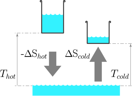
Figure 1: Water-fall picture of Carnot cycles for a system alternately in contact with hot and cold baths, pictured as reservoirs at altitudes $T_{hot}$ and $T_{cold}$, respectively, above a lake. If the cycle is reversible, the amount of water flowing from the upper reservoir to the lake is equal to the amount of water pumped from the lake to the lower reservoir. In that case the Carnot efficiency may be attained. $\Delta\mathrm{S}_{hot}$ and $\Delta\mathrm{S}_{cold}$ represent the entropies produced in the two baths.

The Carnot analogy is illustrated in Fig. 1. Consider a reservoir at altitude $T_{hot}$ above a lake. If some water weight $-\Delta\mathrm{S}_{hot}$ flows from the reservoir to the lake the work performed is $-\Delta\mathrm{Q}_{hot}=-T_{hot}\Delta\mathrm{S}_{hot}$. Consider another reservoir at a lower altitude $T_{cold}$. In order to pump a water weight $\Delta\mathrm{S}_{cold}$ from the lake to the reservoir a work $T_{cold}\Delta\mathrm{S}_{cold}$ is needed. The net work performed $\Delta\mathrm{W}=-T_{hot}\Delta\mathrm{S}_{hot}-T_{cold}\Delta\mathrm{S}_{cold}$ may fluctuate from cycle to cycle. The efficiency is defined as the ratio of the average work performed and the average consumption of heat from the hot bath: $\eta\equiv-\Delta W/\Delta Q_{hot}=1+T_{cold}\Delta S_{cold}/T_{hot}\Delta S_{hot}$. The limiting Carnot efficiency quoted above obtains if $\Delta S_{hot}+\Delta S_{cold}=0$, that is, if the average amount of water lost by the upper reservoir ends up in the lower one.

To conclude that the efficiency may not exceed $\eta_{C}=1-T_{cold}/T_{hot}$, one must prove that the total average bath entropy produced never decreases, that is: $\Delta S_{cold}+\Delta S_{hot}\geq 0$. A concise argument is as follows: In the case of heat pumps we have: $\Delta S_{hot}\geq 0$ and $\Delta S_{cold}\leq 0$. Let us consider the special case for which $T_{cold}\Delta S_{cold}+T_{hot}\Delta S_{hot}=0$, in which case no work is involved ($\Delta W=0$). This relation implies that $\Delta S_{cold}+\Delta S_{hot}\leq 0$, since $T_{hot}\geq T_{cold}$, opposite to the one we wish to prove. But the situation just described does not occur because heat never flows from cold to hot baths spontaneously, according to observation. The general result follows from the fact that the temperatures may be specified arbitrarily.

To summarize: if the entropies produced in the hot and cold baths $\Delta\mathrm{S}_{hot}=\Delta\mathrm{Q}_{hot}/T_{hot}$ and $\Delta\mathrm{S}_{cold}=\Delta\mathrm{Q}_{cold}/T_{cold}$ can be evaluated, the work performed by the engine

$$\Delta\mathrm{W}=-\Delta\mathrm{Q}_{hot}-\Delta\mathrm{Q}_{cold}$$ (1)

is readily obtained since the bath temperatures are known. This work may fluctuate. We are mostly interested in its average value $\Delta W$. The efficiency

$$\eta=1+\frac{\Delta Q_{cold}}{\Delta Q_{hot}}=1+\frac{T_{cold}}{T_{hot}}\frac{\Delta S_{cold}}{\Delta S_{hot}}$$ (2)

reaches the Carnot efficiency when the cycle is reversible, that is, when the total average bath entropy produced per cycle $\Delta S_{hot}+\Delta S_{cold}$ vanishes.

Two seemingly independent entities were considered above, namely the absolute temperature $T$ of a bath, analogous to a reservoir height, and a state function $\mathrm{S}$, called entropy, analogous to the total weight of water contained in a reservoir. To proceed further, we need introduce another state function, namely the energy $\mathrm{U}_{bath}$ contained in the bath. It is plausible that $\mathrm{S}$ be some function of $\mathrm{U}_{bath}$, since both are state functions and no other parameter is presently involved. If an amount of heat $\Delta\mathrm{Q}\ll\mathrm{U}_{bath}$ is added, the bath energy gets incremented by $\Delta\mathrm{U}_{bath}=\Delta\mathrm{Q}$, according to the law of equivalence of heat and energy. The bath entropy gets incremented by $\Delta\mathrm{S}=\beta\leavevmode\nobreak\ \Delta\mathrm{Q}=\beta\leavevmode\nobreak\ \Delta\mathrm{U}_{bath}$, if the inverse bath temperature $\beta\equiv 1/T$ is introduced.

Carnot explained how reversible heat engines could be constructed: He first observed that two bodies should be put into thermal contact only if their temperatures almost coincide. Reversible transformations must be quasi-static, that is, close to an equilibrium state at every instant. As a consequence, ideal heat engines, while efficient, are slow. Reversible heat engines involve four steps, two of them with the system being isolated from the baths (adiabatic transformations), and two of them with the system being in contact with either the hot or the cold baths (isothermal transformations). These four steps will be discussed in detail in subsequent sections.

In the 19th century only systems involving many microscopic degrees of freedom, such as gas-filled cylinders terminated by movable pistons, were considered. We discuss here instead single-mode oscillators that possess a single degree of freedom, the phase of the oscillation being ignored. The conditions under which the cycle should be considered reversible will need clarification. Carnot cycles involving oscillators were discussed before (see [6], and the references therein). Small mechanical systems have been considered, e.g., in [7], and the Statistical Mechanical properties of small electronic systems are discussed, e.g., in [8]. The forces involved in single-mode oscillators are tiny. But rotating-vibrating molecules and biological systems submitted to baths at different temperatures may retrieve energy through Carnot cycles or related devices [9].

The general expression of the work performed by a system in contact with a bath when its parameter varies [10] is recalled in Section 2. It is shown in Section 3 that for linear oscillators at frequency $\omega$ the Carnot result amounts to asserting that the average oscillator action, $f(x)$, is a decreasing function of $x\equiv\beta\omega$. The properties of Carnot cycles for oscillators are discussed in Section 4. The explicit form of $f(x)$ is obtained in Section 5 from a simple prescription. The average work $\Delta W$ performed per cycle and the efficiency $\eta$ are illustrated for reversible and non-reversible cycles in Section 6.

Szilard noted in 1925 that: “exploitation of the fluctuation phenomena will not lead to the construction of a perpetual mobile of the second kind” [11]. It may be shown on the basis of the Boltzmann formulation that the variance as well as the average value of the entropy produced vanish when the reversibility conditions are fulfilled, in agreement with that quotation.

The Boltzmann constant $k_{\mathrm{B}}$, set equal to unity for brevity, is restored in numerical applications. The angular frequency $\omega$ is called “frequency” for short, the Planck constant divided by $2\pi$, $\hbar$, is called “Planck constant”, and the action divided by $2\pi$, namely $\mathrm{f}=\mathrm{U}/\omega$, is called “action”.

2 Work performed by a system in contact with a bath

Let a system depending on a parameter $\omega$ (perhaps the system volume) interact weakly with a bath. Some energy flows between the bath and the system. Eventually a state of equilibrium is reached. The system average energy, denoted $U(\omega,\beta)$, depends on $\omega$ and on the bath inverse temperature $\beta$.

If the parameter varies by $d\omega$, the elementary average work $dW$ performed by the system is written as $dW=-f\,d\omega$, where $f$ is a generalized force. If $\omega$ represents the volume of a gas-filled enclosure, $-f$ represents the gas pressure. If $\omega$ represents an oscillator frequency, $f$ represents the oscillator action. Purely mechanical considerations, such as the law of conservation of momentum, often enable one to evaluate the generalized force as some function $f(\omega,U)$ of $\omega$ and the average system energy $U$. Considering $U$ as a function of $\omega$ and temperature reciprocal $\beta$, as said above, we may view $f$ as a function of $\omega$ and $\beta$ according to $f(\omega,\beta)\equiv f(\omega,U(\omega,\beta))$. In the present paper the parameter $\omega$ is supposed to be prescribed from the outside, that is, it is not subjected to fluctuations. Bath temperatures are of course fixed quantities.

The fact that the bath entropy $S$ is a state function restricts admissible functions $U(\omega,\beta)$. Indeed, the bath entropy increment $dS=\beta dQ=-\beta(dW+dU)\equiv\beta(fd\omega-dU)$, if the law of conservation of energy ($dQ+dW+dU=0$) and the definition of $f$ are introduced. $dS$ may be expressed as

$$dS=\beta(f-\frac{\partial U}{\partial\omega})d\omega-\beta\,\frac{\partial U}{\partial\beta}\,d\beta.$$ (3)

Because $dS$ is a total differential, the derivative with respect to $\omega$ of the term that multiplies $d\beta$ must be equal to the derivative with respect to $\beta$ of the term that multiplies $d\omega$. After simplification, we obtain

$$\frac{\partial U}{\partial\omega}=\frac{\partial(\beta f)}{\partial\beta}.$$ (4)

Since $dW=-f\leavevmode\nobreak\ d\omega$, the work $\Delta W_{isothermal}$ performed by the system in contact with the bath when the parameter varies from $\omega_{in}$ to $\omega_{out}$ is given by

$$\beta\Delta W_{isothermal}(\beta)=-\beta\int_{\omega_{in}}^{\omega_{out}}f(\omega,\beta)d\omega=\phi(\omega_{in},\beta)-\phi(\omega_{out},\beta).$$ (5)

where we have defined

$$\phi(\omega,\beta)\equiv\beta\int^{\omega}f(\omega^{\prime},\beta)d\omega^{\prime}.$$ (6)

The evolution of a system in contact with a bath may be pictured as a sequence of elementary adiabatic evolutions with $\omega$ being incremented by $d\omega$, followed by returns to thermal equilibrium at constant $\omega$. Because the successive steps are statistically independent, the average values and variances of the elementary works performed during the adiabatic steps add up. It follows that the ratio of the standard deviation (square root of the variance) to the average work goes to zero as $1/\sqrt{N}$ when the number $N$ of elementary steps increases. In other words, the work produced may be considered as a non-fluctuating quantity provided the process is sufficiently slow.

3 Linear oscillators

For concreteness, let us consider an inductance-capacitance $\mathcal{L}-\mathcal{C}$ circuit resonating at angular frequency $\omega$, as shown in Figs. 2a and 2b. The electrical charges on the capacitor plates oscillate sinusoidally in the course of time, but the two plates always attract each others. It follows from the Coulomb law that the cycle average force $\mathcal{F}=\mathrm{U}/2a$, where $\mathrm{U}$ denotes the resonator energy and $a$ the capacitor plates separation. If $a$ is incremented by $da$ slowly so that the oscillation remains almost sinusoidal, the elementary work performed by the oscillator is $d\mathrm{W}=-\mathcal{F}\,da=\mathrm{U}\,da/2a$. On the other hand, it follows from the well-known resonance condition $\mathcal{L}\,\mathcal{C}\,\omega^{2}=1$ and the fact that $\mathcal{C}\propto 1/a$, where $\propto$ denotes proportionality, that $2\,d\omega/\omega=da/a$. The elementary work may therefore be written as $d\mathrm{W}=-(\mathrm{U}/\omega)\leavevmode\nobreak\ d\omega\equiv-\mathrm{f}\leavevmode\nobreak\ d\omega$, where we have introduced the generalized force $\mathrm{f}=\mathrm{U}/\omega$. For the average values we have $f=U/\omega$.

When the system is isolated, i.e., not in contact with a heat bath, we have $d\mathrm{Q}=0$ and thus $d\mathrm{U}+d\mathrm{W}=0$. According to the previous expression of $d\mathrm{W}$ the oscillator energy gets incremented by $d\mathrm{U}=(\mathrm{U}/\omega)\,d\omega$. It follows that when the resonant frequency of an isolated oscillator varies slowly, the ratio $\mathrm{U}/\omega$, called “action”, does not vary significantly. In other words, the generalized force $\mathrm{f}=\mathrm{U}/\omega$ is constant in adiabatic processes in the case of oscillators.

Replacing $U$ in (4) by $\omega f$, we obtain after simplification

$$\omega\,\frac{\partial f}{\partial\omega}=\beta\,\frac{\partial f}{\partial\beta},$$ (7)

a relation that entails that $f$ is a function of $\ln(\omega)+\ln(\beta)=\ln(\beta\omega)$ only. This is essentially the displacement law discovered by Wien in 1893 [12]: blackbody spectra scale in frequency in proportion to temperature .

Since $f$ is a function of $\beta\omega\equiv x$ only, the $\phi$-function defined in (6) may be written as

$$\phi(\omega,\beta)=\beta\int^{\omega}f(\omega^{\prime},\beta)\,d\omega^{\prime}=\int^{x}f(x^{\prime})\,dx^{\prime}\equiv\phi(x).$$ (8)

4 The Carnot cycle

Let us first consider the adiabatic processes. Let $\mathrm{U}_{1}$ denote the oscillator energy when it is separated from the hot bath. If the frequency is changed slowly from $\omega_{1}$ to $\omega_{2}$, we have

$$\mathrm{U}_{2}=\frac{\omega_{2}}{\omega_{1}}\mathrm{U}_{1}\equiv\omega_{2}\mathrm{f}_{1},$$ (9)

since isolated oscillator energies are proportional to frequency. Likewise,

$$\mathrm{U}_{4}=\frac{\omega_{4}}{\omega_{3}}\mathrm{U}_{3}\equiv\omega_{4}\mathrm{f}_{3}.$$ (10)

Using the results (5)-(6), (8)-(10), the entropies produced in the hot and cold baths read respectively

$$\beta_{hot}\Delta\mathrm{Q}_{hot} = \beta_{hot}(\mathrm{U}_{4}-\mathrm{U}_{1}-W_{isothermal}(\beta_{hot}))$$ (11)

$$= (a_{4}\mathrm{f}_{3}-\phi(a_{4}))-(a_{1}\mathrm{f}_{1}-\phi(a_{1}))$$

and

$$\beta_{cold}\Delta\mathrm{Q}_{cold} = \beta_{cold}(\mathrm{U}_{2}-\mathrm{U}_{3}-W_{isothermal}(\beta_{cold}))$$ (12)

$$= (a_{2}\mathrm{f}_{1}-\phi(a_{2}))-(a_{3}\mathrm{f}_{3}-\phi(a_{3})),$$

where we have defined

$$a_{1} \equiv\beta_{hot}\omega_{1}, a_{2} \equiv\beta_{cold}\omega_{2}, a_{3} \equiv\beta_{cold}\omega_{3}, a_{4} \equiv\beta_{hot}\omega_{4}.$$ (13)

The above expressions of the $\Delta\mathrm{Q}$ follow simply from the law of conservation of energy. Recall that in these expressions $W_{isothermal}$ is a non-fluctuating quantity.

The average entropies produced are obtained by replacing in (11) and (12) $\mathrm{f}_{1}$ by $f(a_{1})$ and $\mathrm{f}_{3}$ by $f(a_{3})$:

$$\beta_{hot}\Delta Q_{hot} = s(a_{4},a_{3})-s(a_{1})$$

$$\beta_{cold}\Delta Q_{cold} = s(a_{2},a_{1})-s(a_{3}),$$ (14)

where we have introduced a function of two variables

$$s(x,y)\equiv x\,f(y)-\phi(x)\equiv x\,f(y)-\int^{x}f(x^{\prime})\,dx^{\prime},$$ (15)

and $s(x)\equiv s(x,x)$. Note for later use that the function $s(x,y)$ is unaffected by the addition of a constant to $f$. We further observe that $s(x,y)-s(y)\geq 0$ if $f$ is a decreasing function of its argument. We will later on show that this condition, equivalent to the Carnot principle, indeed holds. The average work performed by the system per cycle and the efficiency follow from (14) according to the general expression (1) and (2) if the function $f(x)$ is known. The Carnot efficiency is attained when $a_{1}=a_{2}$ and $a_{3}=a_{4}$, that is, when the reversibility conditions

$$\frac{T_{cold}}{T_{hot}}=\frac{\omega_{2}}{\omega_{1}}=\frac{\omega_{3}}{\omega_{4}}$$ (16)

hold. It is interesting that this condition is independent of the form of the $f(x)$ function.

The total average bath entropy produced per cycle is

$$\Delta S_{t} = \beta_{cold}Q_{cold}+\beta_{hot}Q_{hot}=s(a_{2},a_{1})-s(a_{1})+s(a_{4},a_{3})-s(a_{3})$$ (17)

This quantity is non-negative if $f(x)$ is a decreasing function of $x$, according to a previous remark. For small departures from reversibility, i.e., for $a_{1}\approx a_{2},a_{3}\approx a_{4}$, expansion up to second order of the above expression gives

$$\Delta S_{t}\approx-\frac{1}{2}(a_{2}-a_{1})^{2}\frac{df(a_{1})}{da_{1}}-\frac{1}{2}(a_{4}-a_{3})^{2}\frac{df(a_{3})}{da_{3}}$$ (18)

The Boltzmann-Gibbs formulation tells us that the probability that the system energy be $\epsilon_{k}(\omega)$, $k=0,1\ldots$, is proportional to $\exp(-\beta\epsilon_{k}(\omega))$. One can prove from that formulation that $-df/dx$ is equal to the variance of the oscillator action and is therefore positive. This relation shows further that the variance of the total entropy produced per cycle is twice the average value given in (18), a conclusion related to the ones given in [16] and [17]. These two papers consider only classical systems in contact with a bath, but they are much more general on other respects.

Furthermore, it can be shown that cycles are reversible if and only if

$$\frac{T_{cold}}{T_{hot}}=\frac{\epsilon_{k}(\omega_{2})-\epsilon_{0}(\omega_{2})}{\epsilon_{k}(\omega_{1})-\epsilon_{0}(\omega_{1})}=\frac{\epsilon_{k}(\omega_{3})-\epsilon_{0}(\omega_{3})}{\epsilon_{k}(\omega_{4})-\epsilon_{0}(\omega_{4})},$$ (19)

for $k=1,2,\ldots$. These relations may hold when the $\epsilon_{k}(\omega)$ factorize as $h(k)g(\omega)$. For oscillators in particular we have $\epsilon_{k}(\omega)=(k+1/2)\hbar\omega$, according to the Quantum Optics formulation, and the simpler expression in (16) is recovered. The above result is based on the concept of relative entropy [18]. The mathematical details will be given elsewhere.

5 Average oscillator energy

According to the Boltzmann-Gibbs formulation, the average energy of a classical one-dimensional oscillator is $U=T$. Thus, the average oscillator action $f=1/\beta\omega\equiv 1/x$ obeys the differential equation

$$\frac{df}{dx}+f^{2}=0.$$ (20)

The relation $U=T$, however, is unacceptable because it would necessarily lead to infinite blackbody radiation energy if the Maxwell electromagnetic theory is to be upheld. Indeed, the Maxwell theory applied to a cavity having perfectly conducting walls predicts that there is an infinite number of modes, each of them being modeled as an harmonic oscillator. If an average energy $T$ is ascribed to them, the total energy is clearly infinite. This observation, made near the end of the 19th century, caused a major crisis in Physics [19]. It apparently did not occur to the physicists facing that problem that the mere addition of a constant on the right-hand-side of (20) would solve the problem. Let us indeed suppose that

$$\frac{df}{dx}+f^{2}=\left(\frac{\hbar}{2}\right)^{2}.$$ (21)

where $\hbar$ is now known as the Planck constant. Note that $f$ and $\hbar$ have the dimension of action (‘energy’ $\times$ ‘time’), while $x$ has the dimension of an action reciprocal, so that $\hbar x$ is dimensionless.

The solution of (21) that gives $f(x)-1/x\to 0$ in the classical limit $T\to\infty$ reads

$$f(x)=\frac{\hbar}{2}+\frac{\hbar}{\exp(\hbar x)-1}.$$ (22)

This is the expression obtained by Planck in 1900 from a fit to the available experimental results, aside from the term $\hbar/2$. The latter term is responsible for the Casimir effect [20], [21] but, as we have seen, it does not affect cyclic operations. We obtain from (22) after integration

$$\phi(x)=\frac{\hbar x}{2}+\ln\left[1-\exp(-\hbar x)\right],$$ (23)

Therefore, the entropic function defined in (15) reads

$$s(x,y)=\frac{\hbar x}{\exp(\hbar y)-1}-\ln\left[1-\exp(-\hbar x)\right].$$ (24)

When this result is introduced in (14), explicit expressions for the work performed (1) and efficiency (2) follow. In the classical regime, $T\to\infty$, the above expression reduces to

$$s(x,y)=\frac{x}{y}-\ln(\hbar x).$$ (25)

Note that the Planck constant $\hbar$ cancels out in the final formulas. We leave it there for aesthetic reasons, the argument of $\ln(.)$ being expected to be dimensionless.

The quantities of interest in a Carnot cycle, i.e., mainly the work performed and the efficiency, have been obtained without giving any consideration to the oscillator entropy or temperature. We only need evaluate the entropies produced in the cold and hot baths. For purposes of illustration (see Fig. 2) it is, however, of some interest to introduce the oscillator inverse temperature $\beta_{osc.}$. When the oscillator is in contact with a bath at inverse temperature $\beta$ we have $\beta_{osc.}=\beta$. When the oscillator is isolated and the frequency varies slowly the product $x=\beta_{osc.}\omega$ remains constant, as we have seen. The average system entropy is a function of $x\equiv\beta_{osc.}\omega$ only, and thus remains constant during the adiabatic process. The condition $a_{1}=a_{2}$ stated above amounts to saying that reversibility requires that the oscillator be put into contact with the cold bath only if its inverse temperature is almost equal to $\beta_{cold}$, and likewise for the other adiabatic process. Let us emphasize, however, that this simple picture, similar to the one advanced by Carnot in 1824, does not generally apply to multimode oscillators, unless the modes frequencies vary in proportion of one another, or are continuously thermalized through some non-linear coupling.

6 Illustration of Carnot cycles.

Let us give first an order of magnitude of the work performed, considering for simplicity the classical limit: $T\to\infty$. In that limit: $s(x)=-\ln(x)+\mathrm{constant}$. It follows that for reversible classical cycles the average work performed per cycle reads

$$\Delta W=k_{\mathrm{B}}(T_{hot}-T_{cold})\ln\left(\frac{\omega_{3}}{\omega_{1}}\frac{T_{hot}}{T_{cold}}\right),$$ (26)

where the Boltzmann constant has been restored. At room temperature the classical approximation is a valid one if the oscillator frequencies are substantially smaller than about 10 THz. For example, for $N=1/k_{\mathrm{B}}\approx 10^{23}$ independent oscillators, $T_{hot}=1200$ K, $T_{cold}=300$ K, and $\omega_{1}=2\omega_{3}$, the work done per cycle $\Delta W=900\ln(2)$ J $\approx 620$ J.

Let us now go back to the quantum regime and evaluate explicitly the work performed and the efficiency of oscillators alternately in contact with a hot bath at temperature $T_{hot}=1$ and a cold bath at temperature $T_{cold}=1/4$. We consider in Fig. 2 the case where $\omega_{1}=1$, $\omega_{2}=1/4$, $\omega_{4}=2$ and $\omega_{3}$ is kept as a parameter. When $\omega_{3}=1/2$, the system is reversible and the cycle in the oscillator temperature-versus-entropy diagram in Fig. 2a is rectangular. The entropy $\Delta S_{cold}$ produced in the cold bath is shown by the lower right-directed arrow, while the entropy $-\Delta S_{hot}$ removed from the hot bath is shown by the upper, left-directed arrow. The total produced entropy vanishes in that case. The case of an irreversible cycle with $\omega_{3}=1$ is shown in Fig. 2b. Note the temperature-entropy jump, shown by a dashed line, when the oscillator is put in contact with the hot bath. In that situation the total produced entropy (see the arrows) is positive.

Figure 3a shows how the work performed $\Delta W$ and the efficiency $\eta$ vary as a function of $\omega_{3}$. The Carnot efficiency $\eta_{C}=3/4$ is reached for $\omega_{3}=1/2$. For larger $\omega_{3}$-values the energy extracted per cycle increases but the efficiency is somewhat reduced.

A case of interest is when the resonator frequency is a constant $\omega_{1}$ when the resonator is in contact with the hot bath and a constant $\omega_{2}$ when it is in contact with the cold bath, in which case $a_{1}=a_{4}$ and $a_{2}=a_{3}$. In that situation, the hot and cold baths may be modeled as large collections of oscillators at frequencies close to $\omega_{1}$ and $\omega_{2}$, respectively. Supposing again that $T_{hot}=1$ and $T_{cold}=1/4$. We find from previous expressions that the energy extracted per cycle is maximum when $\omega_{1}=1/2$ and $\omega_{2}=1/4$. For these parameter values the efficiency is $\eta=1/2$, that is, substantially less than the Carnot efficiency $\eta_{C}=3/4$. The variations of the work done and the efficiency as functions of $\omega_{1}$ are shown in Fig. 3b.

Another case of interest is when the parameter does not vary when the system is transferred from one bath to another. In that case, according to the observation that follows (6), the work performed does not fluctuate.

7 Conclusion

We have shown that heat engines whose system is a single-mode linear oscillator obey the Carnot theory. Explicit expressions for the work performed per cycle and the efficiency were obtained on the basis of a simple prescription. We have illustrated reversible and non-reversible cycles, and shown that the variance of the entropy production per cycle vanishes when the cycle is reversible and is, in general, equal to twice the average value.

The present theory may be generalized to multimode oscillators by adding up modal contributions. Consider in particular a non-dispersive transmission line terminated by a movable short-circuit, a configuration resembling the classical gas-filled cylinder with a piston. Because the resonant frequencies change in proportion to one another when the length of the transmission line is modified, a temperature may be defined at every step of the adiabatic process and the Carnot efficiency may be attained. This is also the case when the shape of a cavity does not change as the volume varies. But this is not so for dispersive transmission lines such as waveguides. Slow length changes create an average distribution among the modes that cannot be described by a temperature, unless some thermalization mechanism is enforced at each elementary step. Carnot cycles for radiation are discussed in [22].

The force $f$ depends on the term $\hbar\omega/2$ in the expression of the mode average energy, and is non-zero even at $T=0$K. But if we are only interested in the average work performed over a full cycle, this term may be ignored.

Recent interesting generalizations take into account finite interaction times, $\Delta t$, between the oscillator and the baths. In that case there are departures of the work done from the change in free energy, which are inversely proportional to $\Delta t$. Note also that the energy required to detach a system from a bath should be accounted for when the cycle is not slow [6].

8 Acknowledgments

The authors wish to express their thanks to E. Clot and J.C. Giuntini for a critical reading of the manuscript.

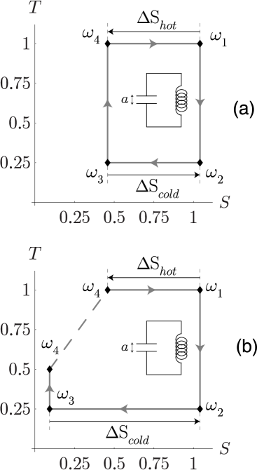
Figure 2: An $\mathcal{L}-\mathcal{C}$ single-mode oscillator is shown. The figure shows cycles in the temperature versus oscillator entropy diagram for the case where $T_{hot}=1$ and $T_{cold}=1/4$, $\omega_{1}=1$, $\omega_{2}=1/4$, $\omega_{3}=c/2$, $\omega_{4}=2$. (a) Reversible cycle, $c$=1. (b) Non-reversible cycle, $c$=2. The horizontal arrows give the average entropies produced in the cold (lower) and hot (upper) baths.

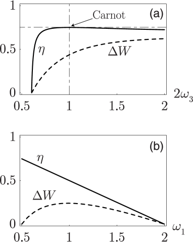
Figure 3: Average work performed per cycle $\Delta W$ and efficiency $\eta$ for $T_{hot}=1$ and $T_{cold}=1/4$, (a) as functions of $2\omega_{3}$. The Carnot efficiency is attained when $2\omega_{3}=1$. (b) The oscillator frequency is kept constant when in contact with either bath. We have set: $\omega_{2}=\omega_{3}=1/4$. $\omega_{1}=\omega_{4}$ is kept as a parameter.

References

- [1] D.V. Schroeder “An introduction to Thermal Physics”, Addison-Wesley, San Francisco, 2000).
- [2] L. Landau et E. Lifchitz “Physique Statistique”, Mir, Moscou (1984), p.66.
- [3] N.S. Carnot, Réflexions sur la puissance motrice du feu (An english translation may be found in: Dover publ. Inc. New-York, 1960).
- [4] “Sadi Carnot et l’essor de la Thermodynamique”, Editions du CNRS, Paris, 1976.
- [5] M.W. Zemansky “Carnot cycle”, in: Encyclopedia of Physics (VCH Publ., New-York, 1990), p.119.
- [6] K. Sekimoto, F. Takagi and T. Hondou, “Carnot’s cycle for small systems: irreversibility and cost of operation”, Phys. Rev. E, 62, 7759-7768 (2000).
- [7] F.M. Serry, D. Wallister and G.J. Maclay “The role of the Casimir effect in the static deflection and striction of membrane strips in microelectro-mechanical systems”, J. of Applied Phys. 84 (5), 2501-2506 (1998).
- [8] J. Arnaud, L. Chusseau and F. Philippe, “Fluorescence from a few electrons”, Phys. Rev. B, 62, 13482–13489 (2000), cond-mat/0103295
- [9] P. Reimann, “Brownian motors: noisy transport far from equilibrium”, cond-mat/0010237. To appear in: Physics Reports.
- [10] C. Kittel and H. Kroemer, Thermal Physics (Freeman, San Francisco, 1980).
- [11] L. Szilard “On the extension of phenomenological Thermodynamics to fluctuation phenomena”, Zeits. Physik 32, 753 (1925).
- [12] W. Wien “Eine neue beziehung der strahlung schwarzer korper zum zweiten hauptsatz der warmetheorie”, Berl.Ber. 55-62 (1893).
- [13] J. Arnaud, Beam and Fiber Optics, Acad. Press, New-York (1976), pp. 42 and 251.
- [14] O. Darrigol, From c-numbers to q-numbers (Univ. of Cal. Press., Berkeley, 1992).
- [15] D.C. Cole “Thermodynamics of blackbody radiation via Classical Physics for arbitrarily-shaped cavities with perfectly reflecting walls”, Foundations of Physics 30 (11), 1849-1867 (2000).
- [16] G.E. Crooks “Entropy production fluctuation theorem and the nonequilibrium work relation for free energy differences”, Phys. Rev. E, 60, 2721–2726, (1999), cond-mat/9901352.
- [17] C. Jarzynski “Nonequilibrium equality for free-energy differences”, Phys. Rev. Lett. 78, 2690–2693, (1997), cond-mat/9610209.
- [18] H. Qian “Relative entropy: free energy associated with equilibrium fluctuations and non-equilibrium deviations”, Phys. Rev. E, 63, 042103/1-4 (2001), math-phys/0007010.
- [19] T.S. Kuhn, Black-body theory and the quantum discontinuity, 1894-1912. (Univ. of Chicago press, Chicago, 1987).
- [20] J.H. Cooke “Casimir force on a loaded string”, Amer. J. of Phys. 66, 569-572 (1998).
- [21] M. Revzen, R. Opher, M. Opher and A. Mann, “Casimir entropy”, J. Phys. A: Math. Gen. 30 (1997) 7783-7789.
- [22] M.H. Lee “Carnot cycle for photon gas?”, Amer. J. of Phys. 69, 874-878 (2001).