Atom gratings produced by large angle atom beam splitters.

Abstract

An asymptotic theory of atom scattering by large amplitude periodic potentials is developed in the Raman-Nath approximation. The atom grating profile arising after scattering is evaluated in the Fresnel zone for triangular, sinusoidal, magneto-optical, and bichromatic field potentials. It is shown that, owing to the scattering in these potentials, two groups of momentum states are produced rather than two distinct momentum components. The corresponding spatial density profile is calculated and found to differ significantly from a pure sinusoid.

PACS number(s): 03.75, 03.75.D, 39.20, 81.16.T

I Introduction

Interaction of atoms with a spatially varying optical field can lead to a spatial modulation of the atomic density. For example, when a collimated atomic beam propagating along the $x$ axis passes through a resonant, standing wave field directed along the $z$ axis, it acquires transverse momentum components $2n\hbar k$ and $\left(2n+1\right)\hbar k$ for the atomic ground and excited states, respectively, where $k$ is the field propagation constant and $n$ is an integer  Interference between these momentum states [1] results in a periodic modulation of the atom density with period $d=\lambda/2,$ where $\lambda=2\pi/k$. This splitting of the atomic wave function (resonant Kapitza-Dirac effect [2]) and the density modulation have been observed in a beam of Na [3] and Ar [4] atoms, respectively. Atom gratings can be deposited on substrates and have potential applications as diffraction gratings for soft x-rays.

The grating density profile $\rho\left(z\right)$ produced by this technique contains an infinite number of Fourier harmonics having periods $\lambda/2n$ and amplitudes $\rho_{n}.$ For the grating profile to be approximately sinusoidal, then at most a few $\rho_{n}$ contribute in the Fourier sum. On the other hand, the ”sharp” grating that can be produced by atom focusing using strong standing wave fields [5, 6] consists of a large number of Fourier components,

$$n\sim\lambda/w\gg 1,$$ (1)

where $w\ll\lambda$ is the spot size of the focussed atoms. Sharp gratings have important lithographic applications, but are not well suited for use as elements to diffract x-rays. For x-ray scattering, one finds that each density component $\rho_{n}$ leads to scattering at angle

$$\theta_{n}=\pm n\lambda_{x}/d,$$ (2)

where $\lambda_{x}\ll\lambda$ is the x-ray wavelength. If one monitors scattering at a specific angle, most of the scattered energy does not contribute to the signal. As a consequence, it is most efficient to scatter x-rays from a sinusoidal atom grating, since only one Fourier component is nonvanishing $\left[n=1\text{ in Eq. (\ref{3})}\right].$ To increase the angle and resolution of scattering one needs a high order sinusoidal grating having period

$$d=\lambda/2\bar{n},$$ (3)

where $\bar{n}>1$. Several techniques have been proposed to produce such high order gratings. One can distinguished two groups of methods, harmonic suppression (HS) and large angle beam splitters (LABS) . In HS, one arrives at a periodicity (3) as a result of suppressing all Fourier components in the atom wave function that are not a multiple of $\bar{n}.$ Included in the HS group are methods that employ photon echoes [7], multicolor fields [8], high order Bragg scattering [9], and Fourier optics techniques [10], methods which are summarized below.

An appropriate echo geometry for HS involves atoms that pass through two standing wave fields, spatially separated by a distance $L$ (or atoms that are subjected to two temporally separated standing wave field pulses). At distances $L^{\prime}=\frac{n^{\prime}}{\bar{n}}L$ ($n^{\prime}>\bar{n}$, where $n^{\prime}$ and $\bar{n}$ are integers having no common factors), the atomic density contains only those Fourier components having $n$ that is a multiple of $\bar{n}.$ The other components are suppressed if the atom beam has a transverse velocity width $\delta\theta>\lambda/L$ [7]. A $\frac{\lambda}{4}-$period grating $\left(\bar{n}=2\right)$ has been observed using this method on ⁸⁵Rb atoms cooled in a MOT and subjected to the 2 time-separated standing wave field pulses [11]. In the multicolor field technique [8], atoms interact during time $\tau$ with a traveling wave field having frequency $\Omega$ and two counterpropagating traveling wave fields having frequencies $\Omega+\delta_{1}$ and $\Omega+\delta_{2}.$ If $\left|\delta_{j}\tau\right|\gg 1$ and the detunings are chosen such as $n_{1}\delta_{1}+n_{2}\delta_{2}=0,$ then a grating having period $\lambda/2\bar{n}$ is produced, with $\bar{n}=n_{1}+n_{2}.$ In contrast to the echo-technique, the multicolor field method allows one to obtain near-unity contrast for arbitrary $\bar{n}.$ For Bragg scattering, a proper choice of the angle between the atomic beam and the field propagation direction or, alternatively, a proper choice of atom-field detunings [12], leads to situations where low spatial harmonics are suppressed. A $\frac{\lambda}{6}-$period grating has been obtained using this technique [9]. In the Fourier optics technique one focuses atoms transmitted through a standing wave field using a long-focus lens. Different harmonics of the atomic wave function are focused at the different positions. Using spatial filtering, one can suppress all harmonics except two, whose interference leads to the grating of the desirable period. In this way one achieves 100% contrast pure sinusoidal gratings, but the amplitude of the gratings decreases with increasing grating order.

An ideal large angle beam splitter (LABS) splits an initial state having transverse momentum $p=0$ into two states having momenta

$$p=\pm\bar{n}\hbar k,$$ (4)

where $\bar{n}\gg 1$. The interference between these states leads to a spatial density

$$\rho\left(z\right)=1+\cos\left(2\bar{n}kz\right)$$ (5)

having period $\lambda/2\bar{n}$. The prototype LABS consists of a V-potential

$$U\left(z,t\right)=f\left(t\right)\hbar k\bar{n}\left|z\right|,$$ (6)

off of which atoms scatter. The function $f(t),$ normalized such that $\int_{-\tau/2}^{\tau/2}f(t)dt=1$, describes the potential experienced by an atom in its rest-frame [$t=x/u,$ where $u$ is the projection of the atom velocity along the beam propagation direction ($x$ axis) and $\tau$ is the pulse duration in the atomic rest frame]. In the Raman-Nath approximation

$$\omega_{\bar{n}k}\tau\ll 1,$$ (7)

where

$\displaystyle\omega_{q}=\hbar q^{2}/2m$

is a recoil frequency and $m$ is the atomic mass, one can show that, at a time $t$ following the atom field interaction and for $\bar{n}\gg\left(\omega_{k}t\right)^{-1/2}$, an atom grating is produced having density

$$\rho\left(z\right) \sim 2\left[1+\cos\left(2\bar{n}kz\right)\right]\text{ \ \ for }\left|z\right|<\bar{n}\frac{\hbar k}{m}t;$$ (8)

$$\sim 1\text{ \ \ for }\left|z\right|>\bar{n}\frac{\hbar k}{m}t.$$ (9)

In the past several years, a number of methods have been proposed for using counterpropagating optical fields to create potentials that simulate a V-potential (6). Atom scattering off these fields involves multiphoton processes that result in a transfer of momentum between the counterpropagating field modes. The effective potential $U\left(z,t\right)$ corresponding to these processes is a function of bi-linear products of the counterpropagating field amplitudes. As a consequence, $U\left(z,t\right)$ has period $\lambda/2$ as a function of $z.$ One might expect that a so-called triangular potential, a periodic potential coinciding with a V-potential within a period,

$$U\left(z,t\right) = f\left(t\right)\hbar k\bar{n}\left\{\begin{tabular}[]{l}-$z,$ for $\left|z\right|<\lambda/8$\\ $z-\lambda/4,$ for $\left|z-\lambda/4\right|<\lambda/8$\end{tabular}\right.,$$ (12)

$$U\left(z+\lambda/2,t\right) = U\left(z,t\right),$$ (13)

should produce gratings similar to the sinusoidal grating (9) produced by the V-potential. Based on this idea several schemes for LABS have been proposed.

The simplest example of such a beam splitter is the strong standing wave field first considered in [2]. After adiabatic elimination of the internal degrees of freedom, one finds a sinusoidal potential having period $\frac{\lambda}{2}$. Asymptotically, for a large potential amplitude, the main contribution to the scattering arises from the area around points $z_{0}$ where the potential slope is maximum; in this region the potential is approximately linear. The momentum an atom acquires after scattering near such points is $p\sim F\tau,$ where $F\sim-\left(\partial U/\partial z\right)_{z=z_{0}}$ is the classical force acting on atom.

An alternative method which produces a potential that more closely approximates (13) is the magneto-optical field geometry [13], in which resonant cross-polarized counterpropagating fields drive a ground-to-excited state transition, $J=0\rightarrow J=1,$ where $J$ is the atomic angular momentum. A magnetic field directed along the $z$ axis that splits the excited state Zeeman sublevels is also applied. A regime has been found where the magneto-optical potential is extremely close to the triangular potential (13). The nonlinearity near $z=z_{0}$ is small compared with that associated with the standing wave potential. Magneto-optical forces have been used to deflect an atomic beam [13] and to split an atomic beam into two momenta components localized near values $p=\pm 21\hbar k$ [$\bar{n}=21$ in Eq. (4)] [14]. Atom scattering from a magneto-optical potential is considered in [15, 16, 17], while the force acting on atoms is calculated in [18]. Instead of using a magnetic field one can detune standing waves symmetrically with respect to the atomic transition frequency [19].

Another way of creating a potential similar to the triangular one is to use a bichromatic field [20], in which atoms scatter from two standing wave fields, shifted from one another with respect to their frequencies, and spatial and temporal phases. Forces resulting from this field have been observed in [21, 22]. A remarkable property of these forces (large magnitude in comparison with radiation forces, insensitivity to atomic velocity) allows for fast atomic beam deceleration [23] and for large angle deflections [24]. The triangular potential associated with a bichromatic field was predicted in [25], and scattering off this field has been observed [26] and studied for two-level [27, 26] and three level atoms [28, 29, 30, 31]. Moreover, it has been shown [32] that atoms can be scattered with unit probability with a given change of momentum if a ”counterintuitive pulse sequence” is used.

Despite the similarity between the triangular potential (13) and V-potential (6), there is an important difference. Owing to the intrinsic $\lambda/2$ periodicity, atoms scatter in the potential (13) not only into states $p=\pm\bar{n}\hbar k$ but also into states having $p=\pm\left(\bar{n}\pm 2\right)\hbar k,$ $\pm\left(\bar{n}\pm 4\right)\hbar k$ $\ldots$. Thus, at best, the potential (13) can produce two groups of momenta centered at $p=\pm\bar{n}\hbar k.$ As such the resulting pattern deviates from that of a true V-potential. The additional momentum states produce deviations from an ideal sinusoidal atom grating (5) by producing additional Fourier components,

$$\rho_{\nu}\left(z\right)=a_{\nu}\cos\left[2\left(\bar{n}+\nu\right)kz\right],$$ (14)

where $\alpha_{\nu}\sim 1$ for $\nu\sim\pm\Delta n/2$ and $\Delta n\ll\bar{n}$ is the range of components created by the potential. Therefore, LABS produces atom gratings that are not pure, high order gratings; their overall periodicity is still $\lambda/2.$ Gratings arising in HS also contain extra terms (14), but one is guaranteed that $a_{\nu}\ll a_{0}$ if $\nu$ is not a multiple of $\bar{n}.$ As a result, atom gratings produced by HS closely approximate high order $\frac{\lambda}{2\bar{n}}$-period gratings, having an envelope that oscillates slightly with period $\lambda/2$ around a constant value.

Scattering into a range of momentum components occurs even for the triangular potential. For potentials which approximate the triangular potential (standing wave, magneto-optical scheme, bichromatic field), additional features arise owing to the nonlinearities in these potentials. It turns out that the width $\Delta n$ for these potentials increases with increasing $\bar{n}.$ If one tries to decrease the grating period by increasing $\bar{n}$, there is a corresponding deterioration of the degree to which the grating profile approximates a pure sinusoidal grating.

In this article we provide a detailed calculation of the spatial gratings produced by LABS, using analytical asymptotic and numerical calculations. We consider only the Fresnel regime when all scattered atomic beams overlap with one another. An asymptotic expression for the atomic wave function in momentum space is derived in the next Section and the atomic density profile is calculated in Sec. 3. Results are summarized and discussed in Sec. 4. In the Appendix, we consider atom gratings produced by the triangular potential (13).

II Atom wave function

In this section, we calculate the atomic response to a standing wave field pulse, a magneto-optical field pulse and a bichromatic field pulse, all in the Raman-Nath approximation. For an atomic beam, the pulsed interaction occurs in the atom rest frame.

A Standing wave.

When a two-level atom interacts with a standing wave field pulse having electric field,

$${\bf E}\left(t\right)={\bf\hat{y}}E_{0}\left(t\right)\cos\left(kz\right)e^{-i\omega t}+c.c.,$$ (15)

having (real) amplitude $E_{0}\left(t\right)$, propagation constant $k$, duration $\tau$, and frequency $\omega$, the atomic wave function ${\bf\Psi}=\left(\begin{tabular}[]{c}$\psi$\\ $\psi_{e}$\end{tabular}\right)$ (in the interaction representation) evolves as

$$i{\bf\dot{\Psi}}=\left(\begin{tabular}[]{cc}0&$\chi\left(t\right)\cos\left(kz\right)\exp\left(i\Delta t\right)$\\ $\chi\left(t\right)\cos\left(kz\right)\exp\left(-i\Delta t\right)$&0\end{tabular}\right){\bf\Psi},$$ (16)

where $\psi$ and $\psi_{e}$ are ground ($g$) and excited ($e$) internal states wave functions, $\Delta=\omega-\omega_{0}$ is the atom-field detuning, $\chi\left(t\right)$=$\mu E_{0}\left(t\right)/\hbar$ is a Rabi frequency, $\omega_{0}$ is the ground to excited state transition frequency, and $\mu$ is a (real) dipole moment operator matrix element associated with the $e\rightarrow g$ transition. In Eq. (16) we neglect a term, $\left(\hat{p}^{2}/2m\hbar\right){\bf\Psi}$, ($\hat{p}$ is the atomic center-of-mass momentum operator), which is valid in the Raman-Nath approximation (7). For an adiabatic pulse

$$\dot{\chi}/\chi\ll\max\left\{\left|\Delta\right|,\left|\chi\right|\right\},$$ (17)

it is convenient to use a semiclassical dressed state approach [33]. If the wave function before the pulse arrives is given by ${\bf\Psi}_{-}=\left(\begin{tabular}[]{c}$\psi_{-}\left(z\right)$\\ $0$\end{tabular}\right),$ then, immediately following the pulse, the atom returns adiabatically to its ground state and the wave function is ${\bf\Psi}_{+}=\left(\begin{tabular}[]{c}$\psi_{+}\left(z\right)$\\ $0$\end{tabular}\right),$ where

$$\psi_{+}\left(z\right) = \eta\left(z\right)\psi_{-}\left(z\right),$$ (19)

$$\eta\left(z\right) = \exp\left[-i\theta\left(z\right)\right],$$ (20)

$$\theta\left(z\right) = \int_{-\infty}^{\infty}dt\left\{\left[\frac{\Delta^{2}}{4}+\frac{\chi^{2}\left(t\right)}{2}\left(1+\cos\left(2kz\right)\right)\right]^{1/2}-\frac{\Delta}{2}\right\},$$ (21)

$\eta\left(z\right)$ is a transmission function and $\theta\left(z\right)$ is the spatially inhomogeneous pulse area. To simplify the calculations, it is assumed that the pulses considered in this paper have leading and trailing edges of duration $\tau_{r}$, and that the pulse Rabi frequency is constant and equal to $\chi$ between the leading and trailing edges. Adiabaticity is guaranteed if $\left|\Delta\right|\tau_{r}\gg 1.$ Moreover, if $\tau_{r}/\tau\ll 1,$ the contribution to the phase $\theta\left(z\right)$ from the tails is smaller by a factor of order $\tau_{r}/\tau$ from that of the central region and modifies only slightly the points of stationary phase to be calculated below. As such we approximate $\theta\left(z\right)$ as

$$\theta\left(z\right) = \theta w\left(z\right),$$ (23)

$$w\left(z\right) = \left\{1+\xi\left[1+\cos\left(2kz\right)\right]\right\}^{1/2}$$ (24)

where

$\displaystyle\theta=\Delta\tau/2$

and

$\displaystyle\xi=2\chi^{2}/\Delta^{2}.$

If initially an atom is in the zero momentum state, then the Fourier components

$$\psi_{n}=\int_{0}^{\lambda/2}\frac{dz}{\lambda/2}\exp\left[-2inkz-i\theta(z)\right]$$ (25)

determine the amplitudes for scattering into momentum states $p=2n\hbar k,$ which we refer to as scattering into state $n.$

In the asymptotic limit

$$\theta_{\max}-\theta_{\min}\gg 1,$$ (26)

the main contribution to the integral (25) arises from points of stationary phase, $z=z_{0}.$ These contributions are maximal if the second derivative of the phase also vanishes at $z=z_{0}$. This means that the dominant contribution to scattering into state $n$ occurs for $n\approx\tilde{n}_{0},$ where $\tilde{n}_{0}$ is determined by the equations

$$\tilde{n}_{0} = -\theta^{\prime}\left(z_{0}\right)/2k,$$ (28)

$$\theta^{\prime\prime}\left(z_{0}\right) = 0.$$ (29)

Expanding the phase in (25) to third order in $\left(z-z_{0}\right),$ one finds that $\psi_{n}$ is given by the asymptotic expression,

$$\psi_{n}\sim 2k\left[2/\left|\theta^{\prime\prime\prime}\left(z_{0}\right)\right|\right]^{1/3}\exp\left[-2inkz_{0}-i\theta\left(z_{0}\right)\right]Ai\left\{\Delta n2k\left[2/\theta^{\prime\prime\prime}\left(z_{0}\right)\right]^{1/3}\right\},$$ (30)

where

$\displaystyle\Delta n=n-\tilde{n}_{0}$

and $Ai\left(x\right)$ is an Airy function. For the field parameters given in (II A), one has

$$\tilde{n}_{0} = \pm n_{0};$$ (32)

$$n_{0} = \theta\left\{\left[1+\xi-\left(1+2\xi\right)^{1/2}\right]/2\right\}^{1/2},$$ (33)

$$\theta^{\prime\prime\prime} = \pm 8k^{3}n_{0},$$ (34)

$$z_{0} = \pm\frac{\lambda}{4\pi}\cos^{-1}\left\{\left[\left(1+2\xi\right)-1-\xi\right]/\xi\right\},$$ (35)

$$\theta\left(z_{0}\right) = \theta\left(1+2\xi\right)^{1/4},$$ (36)

such that

$$\left|\psi_{n}\right|^{2}\sim\left(2/n_{0}\right)^{2/3}Ai^{2}\left[\Delta n\left(2/n_{0}\right)^{1/3}\right].$$ (37)

The distribution (37) is plotted in Fig. 1 and has width (full-width at half maximum)

$$\Delta n_{sw}\approx 1.29n_{0}^{1/3}.$$ (38)

The result (37) differs from that obtained in reference [2].

Using an asymptotic expression for the Airy function for large negative arguments one finds that for $\Delta n<0$ and $\left|\Delta n\right|\gg 1$ the distribution oscillates as a function of $\Delta n.$ Averaging over these oscillations one finds

$$\left|\psi_{n}\right|^{2}\sim\pi^{-1}\left(2n_{0}\Delta n\right)^{-1/2}.$$ (39)

which coincides with the momentum distribution associated with classical particles scattered by a standing wave potential [34].

In the case of a far detuned field $\left(\xi\ll 1\right),$ when

$$\theta\left(z\right) = \theta\left\{1+\frac{\xi}{2}\left[1+\cos\left(2kz\right)\right]\right\},$$ (41)

$$n_{0} = \theta\xi/2,$$ (42)

one finds from Eq. (25) that the exact expression for the Fourier harmonics is

$$\psi_{n}=J_{n}\left(\theta\xi/2\right)\exp\left[-in\pi/2-i\theta(1+\xi/2)\right],$$ (43)

where $J_{n}\left(x\right)$ is a Bessel function. The asymptotic result (30) follows directly from Eq. (43) using a well-known asymptotic expression for large order Bessel functions [35]. One can consider Eq. (30) as a generalization of the asymptotic expression for Bessel functions in the limit that $n\gg 1$ for a function having arbitrarily large periodical phase.

B Magneto-optical potential

This regime of scattering arises [13], when atoms interact with an optical field

$${\bf E(}z,t)=E_{0}\left(t\right)\left({\bf\hat{y}}e^{ikz}+{\bf\hat{x}}e^{-ikz}\right)e^{-i\omega t}+c.c.$$ (44)

and a static magnetic field along ${\bf\hat{z}}.$ If the optical field drives a $J=0\rightarrow J=1$ ground-to-excited state transition, then the wave function ${\bf\Psi}^{\prime}{\bf=}\left(\begin{tabular}[]{l}$\psi^{\prime}$\\ $\psi_{-e}$\\ $\psi_{e}$\end{tabular}\right),$ ($\psi^{\prime}=\psi e^{i\Delta t},$ $\psi_{-e},$ $\psi_{e}$ are amplitudes for the ground state, $m_{j}=-1$ excited state, and $m_{j}=1$ excited state, respectively) evolves as

$$i{\bf\dot{\Psi}}^{\prime}{\bf=U\Psi}^{\prime}{\bf,}$$ (45)

where the interaction Hamiltonian is

$$\hbar{\bf U}=\hbar\left(\begin{tabular}[]{ccc}$\Delta$&$G_{-}$&$G_{+}$\\ $G_{-}^{\ast}$&-$\omega_{L}$&$0$\\ $G_{+}^{\ast}$&$0$&$\omega_{L}$\end{tabular}\right),$$ (46)

$\pm\omega_{L}$ are Zeeman shifts of the states $\pm e,$

$\displaystyle G_{\pm}=\mp 2^{-1/2}\omega_{R}e^{\pm i\pi/4}\cos\left(kz\mp\pi/4\right),$

$\omega_{R}=2\times 3^{-1/2}E_{0}^{\ast}\left(t\right)\mu/\hbar$ is a Rabi frequency, and $\mu$ is a reduced matrix element of the dipole moment operator. To develop an asymptotic solution of Eq. (45), one must first solve the characteristic equation

$$\left|U-\lambda I\right|=0.$$ (47)

Solutions can be found in Refs. [15, 16, 18]. Let us denote by $\lambda\left(z,t\right)$ the root of Eq. (47) which equals $\Delta$ when the field vanishes. If initially an atom is in its ground state and if there is no level crossing during the interaction, then after the pulse the atom returns to its ground state. The ground state wave function $\psi$ following the pulse is given by equations analogous to Eqs. (17) with a pulse area defined by

$$\theta\left(z\right)=\int_{-\infty}^{\infty}dt\left[\lambda\left(z,t\right)-\Delta\right].$$ (48)

A potential that closely resembles the triangular potential (6) emerges if one chooses a rectangular pulse having [13]

$$\omega_{R}=2\omega_{L}\text{ and }\Delta=0$$ (49)

(although $\Delta=0$, adiabaticity is still maintained if $\omega_{L}\tau_{r}\gg 1$). For these values, we find from Eqs. (46) and (48) that

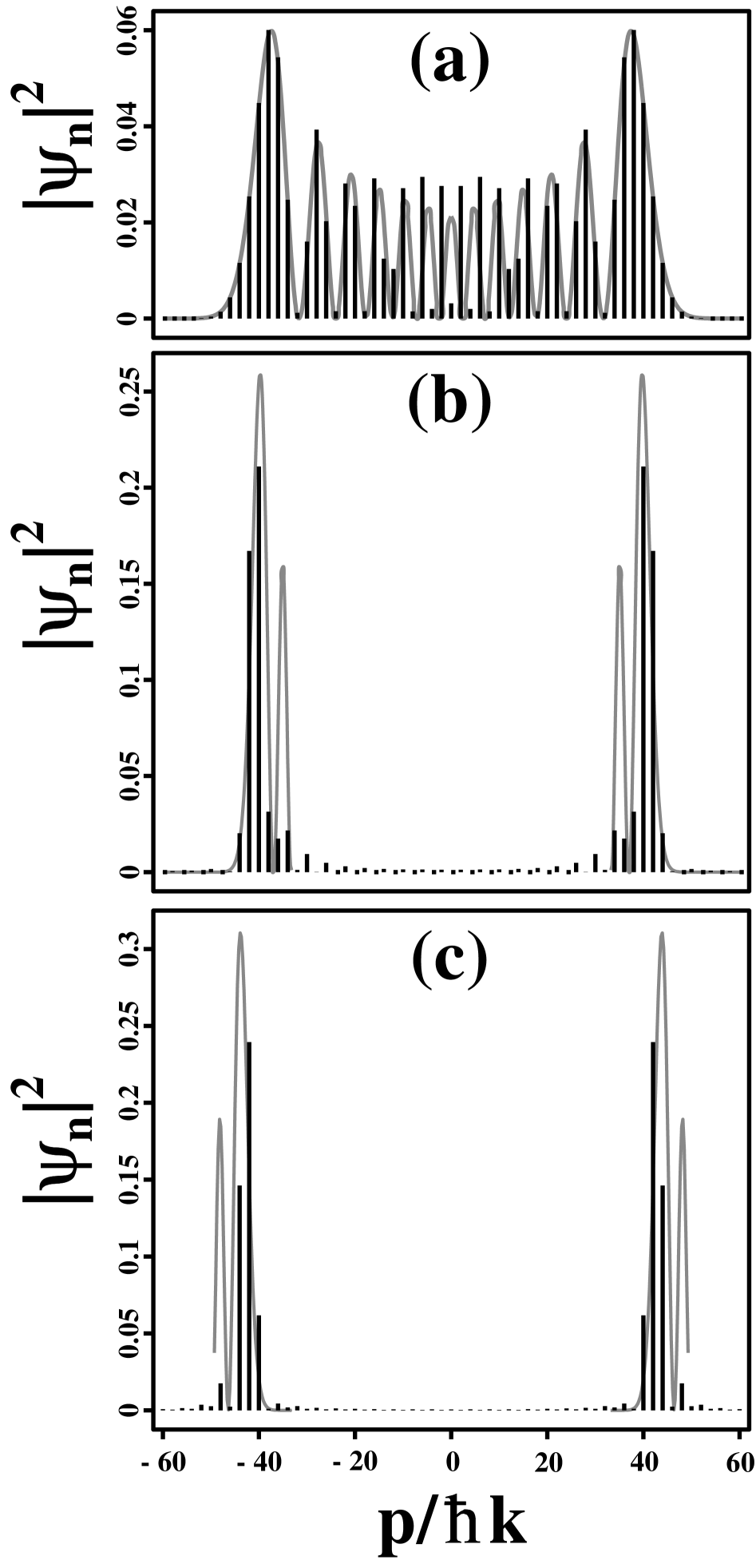
FIG. 1.: Probabilities $\left|\psi_{n}\right|^{2}$ for atom scattering by LABS into momentum states $p=n\hbar k$ located at $n\approx\pm n_{0}$ for $n_{0}=20\pi/3,$ corresponding to the modulation amplitude chosen in [15] for numerical calculations; $\left(a\right)$ standing wave field, $\left(b\right)$ magneto-optical field, $\left(c\right)$ bichromatic field. Solid lines are the numerical values and the gray solid lines are asymptotic expressions obtained from Eqs. (37, 58, 77).

$$\theta\left(z\right) = -\theta w\left(z\right),$$ (51)

$$w\left(z\right) = \sin\left\{\frac{1}{3}\sin^{-1}\left[\sin\left(2kz\right)\right]\right\},$$ (52)

where $\theta=2\omega_{L}\tau.$ The function $w\left(z\right)$ has discontinuous derivatives. In the regions of continuity this function is given by

$$w\left(z\right) = \sin\left(\frac{2}{3}kz\right),\text{ for }0<z<\frac{\lambda}{8},$$ (54)

$$= \sin\left(\frac{\pi-2kz}{3}\right),\text{ for }\frac{\lambda}{8}<z<\frac{3}{8}\lambda,$$ (55)

$$= \sin\left[\frac{2}{3}\left(kz-\pi\right)\right],\text{ for }\frac{3}{8}\lambda<z<\frac{\lambda}{2}.$$ (56)

The slope of $w\left(z\right)$ has extrema at $z_{0}=0$ and $z_{0}=\lambda/4,$ associated with splitting of the incident state in two momentum groups located at $\tilde{n}_{0}=\pm n_{0},$ with

$$n_{0}=\theta/3.$$ (57)

From Eq. (30) it follows that

$$\psi_{n}\sim\left(\pm 1\right)^{n}\left(18/n_{0}\right)^{1/3}Ai\left[\pm\Delta n\left(18/n_{0}\right)^{1/3}\right].$$ (58)

Exact and asymptotic values for $\left|\psi_{n}\right|^{2}$ as a function of $n$ are shown in Fig. 1. One sees that asymptotically, for a given angle of splitting (i. e. a given value of $n_{0}),$ the net result of replacing a standing wave field by a magneto-optical field is to increase the maximum of the scattering probability by a factor $3^{4/3}$ and decrease of the distribution width $\Delta n_{mo}$ by a factor $3^{2/3}.$ In spite of this, the width of distribution is still an increasing function of the angle of scattering,

$$\Delta n_{mo}=0.62n_{0}^{1/3}$$ (59)

C Bichromatic field

Finally, we consider the interaction of a two-level atom with a quantized field composed of two standing wave fields having frequencies $\omega_{0}\pm\Delta,$ the same initial number of photons $\nu\gg 1,$ and shifted with respect to one another by a quarter of a wavelength. The Hamiltonian can be written as [27]

$$H = H_{0}+H_{I},$$ (61)

$$H_{0} = \hbar\omega_{0}\left(\left|e\right\rangle\left\langle e\right|+c^{\dagger}c+d^{\dagger}d\right),$$ (62)

$$H_{I} = \hbar\Delta\left(c^{\dagger}c-d^{\dagger}d\right)-\hbar g\left\{\cos\left(kz+\pi/4\right)\left[c^{\dagger}\left|g\right\rangle\left\langle e\right|+\left|e\right\rangle\left\langle g\right|c\right]+\cos\left(kz-\pi/4\right)\left[d^{\dagger}\left|g\right\rangle\left\langle e\right|+\left|e\right\rangle\left\langle g\right|d\right]\right\},$$ (63)

where $c$ and $d$ are annihilation operators for modes $\omega_{0}\pm\Delta,$ $g$ is a coupling constant, and $H_{I}$ is the interaction Hamiltonian. If initially an atom is in its ground state, then in the interaction representation the system wave function is given by

$${\bf\Psi=}\left(\begin{tabular}[]{c}$\vdots$\\ $\psi_{g}\left(\nu-1,\nu+1;z,t\right)$\\ $\psi_{e}\left(\nu-1,\nu;z,t\right)$\\ $\psi\left(z,t\right)$\\ $\psi_{e}\left(\nu,\nu-1;z,t\right)$\\ $\psi_{g}\left(\nu+1,\nu-1;z,t\right)$\\ $\vdots$\end{tabular}\right),$$ (64)

where $\psi_{i}\left(m,n;z,t\right)$ is the amplitude for the atom to be in state $\left|i\right\rangle$ and the field to be in a state having $m$ and $n$ photons in the modes $\omega_{0}\pm$ $\Delta,$ respectively. Before the atom field interaction, $\psi\left(z,t\right)\equiv\psi_{g}\left(\nu,\nu;z,t\right)$. This wave function evolves as

$$i{\bf\dot{\Psi}} = {\bf L\Psi,}$$ (66)

$${\bf L} = \left(\begin{array}[]{ccccccc}\ddots&&&&&&\\ \Omega_{+}&2\Delta&\Omega_{-}&&&&\\ &\Omega_{-}&\Delta&\Omega_{+}&&&\\ &&\Omega_{+}&0&\Omega_{-}&&\\ &&&\Omega_{-}&-\Delta&\Omega_{+}&\\ &&&&\Omega_{+}&-2\Delta&\Omega_{-}\\ &&&&&&\ddots\end{array}\right),$$ (74)

where $\Omega_{\pm}=\Omega_{0}\cos\left(kz\pm\pi/4\right),\,$and $\Omega_{0}=g\sqrt{\nu}$ is a Rabi frequency. Let us denote by $\lambda\left(z,t\right)$ the eigenvalue of the matrix ${\bf L}$ associated with a dressed state (eigenvector of the matrix ${\bf L)}$ which coincides with the initial state of the system before and after the interaction. As in the cases above, if adiabaticity is maintained, the initial state wave function undergoes a phase shift as a result of the interaction. The final state wave function is still given by Eq. (20), with $\theta\left(z\right)=\int_{-\infty}^{\infty}dt\lambda\left(z,t\right).$

A remarkable situation had been found in reference [25]. With a Rabi frequency $\Omega_{0}=\sqrt{3}\Delta/2,$ $\theta\left(z\right)$ closely approximates a triangular potential. Explicitly, one finds

$$\theta\left(z\right)=-\theta w\left(z\right),$$ (75)

where $\theta=-\Delta\tau$ and the function $w\left(z\right)$ is shown in Fig. 2.

FIG. 2.: One period of the normalized pulse area $w\left(z\right)=\theta\left(z\right)/\theta$ for scattering by a bichromatic field.

The slope of $w\left(z\right)$ has extrema at $z=0$ and $z=\lambda/4,$ where $w^{\prime}\approx\pm 0.624k,$ $w^{\prime\prime\prime}\approx\pm 0.211k^{3}.$ Using these values one finds that atoms scatter in two states near $\tilde{n}_{0}=\pm n_{0},$ with

$$n_{0}\approx 0.312\theta,$$ (76)

The corresponding Fourier components are

$$\psi_{n}\sim\left(\pm 1\right)^{n}2.870\,n_{0}^{-1/3}Ai\left(\mp 2.870\,\Delta n/n_{0}^{1/3}\right).$$ (77)

In this case the distribution $\left|\psi_{n}\right|^{2}$ has width

$$\Delta n_{bc}=0.57n_{0}^{1/3}.$$ (78)

This distribution is plotted in Fig. 1. The distribution, obtained here by a numerical integration of Eq. (25) with pulse area (75), differs from the distribution calculated in the article [27] by a numerical solution of the Shrödinger equation. We suppose that differences arise owing to the fact that a rectangular pulse profile was used in [27]; such a pulse does not satisfy our adiabaticity requirements.

III Atom grating profile

The LABS split an initial $p=0$ state into two groups of states having momenta close to $p=\pm 2n_{0}\hbar k.$ It is of interest to compare the matter gratings generated by these LABS in the Fresnel scattering zone with those of an ideal beam splitter. An ideal beam splitter produces purely sinusoidal gratings having period

$$d_{i}=\lambda/4n_{0}.$$ (79)

At a time $t$ after scattering from a potential having period $\lambda/2,$ each momentum state’s amplitude evolves as $\psi_{n}\exp\left(-i\omega_{2k}n^{2}t\right),$ where $\omega_{2k}=2\hbar k^{2}/m$ is a recoil frequency. The atom density $\rho\left(z,t\right)$ is given by

$$\rho\left(z,t\right)=\sum_{n,n^{\prime}}\psi_{n}\psi_{n^{\prime}}^{\ast}\exp\left[2ikz\left(n-n^{\prime}\right)-i\omega_{2k}t\left(n^{2}-n^{\prime 2}\right)\right].$$ (80)

Asymptotic calculation of the atomic density profile is simplest for a triangular potential (13) (see Appendix). One finds in that case that the grating profiles are not those of an ideal beam splitter. If one wishes to carry out analogous solutions for the potentials considered in Sec. II, purely numerical calculations are needed. Such calculations are not given in this paper.

We are left with the problem of evaluating Eq. (80) in some asymptotic limit. Immediately we run into two problems: (1) Owing to the nonlinearities in the potentials, one cannot simply use the asymptotic expression for the Fourier components (30) since, when these expressions are substituted into Eq. (80), one finds that the constraint,

$$\sum\left|\psi_{n}\right|^{2}=1,$$ (81)

is violated. Equation (81) follows from Eq. (80) and the fact that $2\int_{0}^{\lambda/2}\rho\left(z,t\right)dz/\lambda=1.$ If one restricts the summation to values $n\approx\tilde{n}_{0},$ the series $\sum\left|\psi_{n}\right|^{2}$ calculated using Eq. (80) diverges as $\sum\left(n-\tilde{n}_{0}\right)^{-1/2}.$ This example demonstrates that an alternative technique is needed to calculate the atomic density in the asymptotic limit, which allows one to include contributions from all momentum states. (2) Potentials having smooth rather than triangular extrema lead to the atom focusing [5, 6] at a time $t\sim 1/\theta\omega_{2k}$ [36], i. e. to a sharp $\frac{\lambda}{2}$-period grating having little in common with a sinusoidal grating. There is no simple way to predict the times for which this density pattern is transformed into one that might resemble that of the triangular potential. Rather than looking for such times numerically, we consider an alternative approach for obtaining the grating profile, valid for large times.

To this point we assumed implicitly that we were dealing with a monovelocity atomic beam. The time $t$ is related to the observation plane at a distance $x$ from the interaction zone, by $t=x/u,$ where $u$ is the atom velocity along the $x$-axis. In principle, for a LABS one needs a monovelocity beam, since the pulse area $\theta$ and (therefore) the angle of scattering $\left(n_{0}\right)$ depends on $u$ like $1/u;$ however, one can neglect this dependence for a small width of the velocity distribution, $\Delta u\ll u.$ Although we require $\Delta u\ll u$, it is assumed that $\Delta u$ is nonvanishing such that, for

$$x\gg u^{2}/\Delta u\omega_{2k}$$ (82)

the grating (80) is an oscillating function of $u$ [37]. On averaging over $u$ one finds that the phase factor $\exp\left[-i\omega_{2k}t\left(n^{2}-n^{\prime 2}\right)\right]$ appearing in (80) averages to zero unless [38]

$$n^{\prime}=\pm n.$$ (83)

Gratings of this type have been observed recently in the optical Talbot effect [39].

Setting $n^{\prime}=\pm n$ in Eq. (80) one finds that the overall grating period becomes $\lambda/4,$ instead of $\lambda/2.$ Inside a period of the grating profile $\left(0<z<\lambda/4\right),$ one arrives [38] at the following expression for the density:

$$\rho\left(z,t\right) = B+\Phi\left(z\right),$$ (85)

$$B = \int_{0}^{\lambda/2}\frac{dz}{\lambda/2}\left|\eta\left(z\right)\right|^{2}-\left|\int_{0}^{\lambda/2}\frac{dz}{\lambda/2}\eta\left(z\right)\right|^{2}$$ (86)

$$\Phi\left(z\right) = \frac{1}{2}\left[F\left(z\right)+F\left(z+\lambda/4\right)\right],$$ (87)

$$F\left(z\right) = \int_{\left|\hat{z}\right|<Min\left\{z,\frac{\lambda}{2}-z\right\}}\frac{d\hat{z}}{\lambda/4}\eta\left(z+\hat{z}\right)\eta^{\ast}\left(z-\hat{z}\right),$$ (88)

where $B$ is a constant background of order unity and $\eta\left(z\right)$ is the transmission function defined in Eq. (19). We will refer to $\Phi\left(z\right)$ as the grating profile. Although $\Phi\left(z\right)$ can be negative, the atom density $\rho\left(z,t\right)\$is always positive. For a phase transmission function (20) having symmetric or antisymmetric pulse area $\left[\theta\left(z\right)=\pm\theta\left(-z\right)\right],$ one can simplify Eqs. (87, 88) as

$$\Phi\left(z\right) = \frac{1}{2}\left[F\left(z\right)+F\left(\lambda/4-z\right)\right],$$ (90)

$$F\left(z\right) = \int_{-z}^{z}\frac{d\hat{z}}{\lambda/4}\exp\left[i\theta\chi\left(z,\hat{z}\right)\right],$$ (91)

$$\chi\left(z,\hat{z}\right) = w\left(z+\hat{z}\right)-w\left(z-\hat{z}\right),$$ (92)

where the functions $w\left(z\right)$ characterizing the various potentials have been given in Sec. II.

A Standing wave field

To simplify the calculations, we consider the asymptotic grating profile for a far-detuned standing wave field $\left(\xi=2\chi^{2}/\Delta^{2}\ll 1\right)$ whose pulse area is given by Eq. (41). For this pulse $w(z)=\left\{1+\frac{\xi}{2}\left[1+\cos\left(2kz\right)\right]\right\}$ and

$$\chi\left(z,\hat{z}\right)=\xi\sin\left(2kz\right)\sin\left(2k\hat{z}\right)$$ (93)

For large $n_{0}=\theta\xi/2\gg 1,$ one can evaluate the integral (91) using a stationary phase method. The points of stationary phase are at $\hat{z}=\pm\lambda/8.$ These points belong to the region of integration if $z>\lambda/8.$ Thus, neglecting terms of the order of $1/\theta,$ one finds

$$F\left(z\right)\sim\Theta\left(z-\lambda/8\right)2^{3/2}\left[\pi\theta\xi\sin\left(2kz\right)\right]^{-1/2}\cos\left[\theta\xi\sin\left(2kz\right)-\pi/4\right],$$ (94)

where $\Theta\left(z-\lambda/8\right)$ is a Heaviside step-function. This expression becomes invalid near $z=\lambda/4$; however, for $\lambda/4-z\lesssim\lambda/n_{0}$ the integral (91) can be approximated as

$$F\left(z\right)\sim 2J_{0}\left[\theta\xi\left(\pi-2kz\right)\right]$$ (95)

Substituting Eqs. (94, 95) in (90) one obtains

$$\Phi\left(z\right) \sim J_{0}\left(4n_{0}kz\right),\text{ for }z\lesssim\lambda/n_{0};$$ (97)

$$\sim \left[\pi n_{0}\sin\left(2kz\right)\right]^{-1/2}\cos\left[2n_{0}\sin\left(2kz\right)-\pi/4\right],\text{ for }z\neq 0\text{ and }z\neq\lambda/4;$$ (98)

$$\sim J_{0}\left[2n_{0}\left(\pi-2kz\right)\right],\text{ for }\lambda/4-z\lesssim\lambda/n_{0}.$$ (99)

The profile $\Phi\left(z\right)$ is shown in Fig. 3. For large $n_{0}$ one sees from (98) that $\Phi\left(z\right)$ oscillates rapidly with a spatially inhomogeneous period equal to

$$d\left(z\right)=d_{i}/\cos\left(2kz\right).$$ (100)

Although there are rapid oscillations with reduced periodicity, the grating does not approach the purity associated with an ideal beam splitter.

B Magneto-optical potential.

For the magneto-optical scheme the pulse area, as a function of $z,$ has discontinuous derivatives at multiples of $z=\lambda/8$ [see Eqs. (1, II B)]. Since both arguments $z\pm\hat{z}$ of the $w$-functions in Eq. (92) vary in the interval $\left[0,2z\right]$ for $\left|\hat{z}\right|<z,$ one has to consider 4 cases:

$$\alpha)\,\,z\in\left[0,\lambda/16\right],\,\,\beta)\,\,z\in\left[\lambda/16,\lambda/8\right],\,\,\gamma)\,\,z\in\left[\lambda/8,3\lambda/16\right],\,\,\delta)\,\,z\in\left[3\lambda/16,\lambda/4\right].$$ (101)

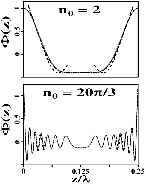
FIG. 3.: Grating profile produced by a far-detuned standing wave field. Solid gray lines are the exact profile calculated using Eqs. (III, 93), dashed and dot-dashed lines are asymptotic results (97, 99) and (98), respectively.

For the simplest case $\alpha)$ one uses expression (54) for both functions $w\left(z\pm\hat{z}\right)$ to find $\chi\left(z,\hat{z}\right)=2\cos\frac{2}{3}kz\sin\frac{2}{3}k\hat{z}.$ Stationary phase points occur for $\hat{z}_{s}=\pm\frac{3}{8}\lambda\notin\left[-z,z\right]$, and one can use an integration by parts in Eq. (91) to arrive at the asymptotic expression

$$F\left(z\right)\sim\left.3\sin\left[\theta\sin\left(\frac{4}{3}kz\right)\right]\right/\pi\theta\cos^{2}\left(\frac{2}{3}kz\right).$$ (102)

We will see below that only for small $z\sim 1/k\theta$ and for $\left|z-\lambda/4\right|\sim 1/k\theta$ will terms of order $\theta^{-1}$ be important. In all other cases terms of order unity (arising for values of $z$ where $\chi\left(z,\hat{z}\right)\sim 1/\theta),$ and terms of order $\theta^{-1/2}$ (arising from integration near stationary phase points) dominate. If such terms are absent, we say that corresponding contribution vanishes.

In case $\beta)$ the function $w\left(z+\hat{z}\right)$ is equal to $\sin\left[\frac{2}{3}k\left(z+\hat{z}\right)\right]$ and $\sin\left[\frac{1}{3}\left(\pi-2k\left(z+\hat{z}\right)\right)\right]$ in the intervals $\hat{z}\in A_{+}=\left[-z,\frac{\lambda}{8}-z\right]$ and $\hat{z}\in B_{+}=\left[\frac{\lambda}{8}-z,z\right]$ respectively, while the function $w\left(z-\hat{z}\right)$ is equal to $\sin\left[\frac{2}{3}k\left(z-\hat{z}\right)\right]$ and $\sin\left[\frac{1}{3}\left(\pi-2k\left(z-\hat{z}\right)\right)\right]$ in the intervals $\hat{z}\in A_{-}=\left[z-\frac{\lambda}{8},z\right]$ and $\hat{z}\in B_{-}=\left[-z,z-\frac{\lambda}{8}\right].$ Since $B_{\mp}\subset A_{\pm}$ one has to map out the region of integration $\left[-z,z\right]$ into 3 intervals:

$$a=\left[-z,z-\frac{\lambda}{8}\right],\,\,b=\left[z-\frac{\lambda}{8},\frac{\lambda}{8}-z\right],\,\,c=\left[\frac{\lambda}{8}-z,z\right].$$ (103)

Let us denote by $F_{i}\left(z\right)$ the contribution to $F\left(z\right)$ from interval $i$ $\left(i=a,\,\,b,\,\,c\right)$ For $\hat{z}\in a,$ $\chi\left(z,\hat{z}\right)=2\sin\left[\frac{1}{6}\left(4kz-\pi\right)\right]\cos\left[\frac{1}{6}\left(\pi+4k\hat{z}\right)\right],$ $\hat{z}_{s}=-\lambda/8\notin a,$ but the function $\chi$ becomes small near $z=\lambda/8,$ i. e.

$$F_{a}\left(z\right) \sim \frac{3}{\pi}\int_{0}^{\pi/6}d\phi\exp\left[-\frac{4}{3}i\theta k\left(\frac{\lambda}{8}-z\right)\cos\phi\right],\text{ for }\frac{\lambda}{8}-z\lesssim 1/k\theta,$$ (105)

$$\sim 0,\text{ otherwise.}$$ (106)

The functions $F_{b}\left(z\right)=0$, $F_{c}\left(z\right)=F_{a}^{\ast}\left(z\right),$ and one finds for case $\beta)$

$$F\left(z\right) \sim J\left[\frac{4}{3}\theta k\left(\frac{\lambda}{8}-z\right)\right],\text{ for }\frac{\lambda}{8}-z\lesssim 1/\theta,$$ (108)

$$\sim 0,\text{ otherwise},$$ (109)

where

$$J\left(\bar{z}\right)=\frac{6}{\pi}\int_{0}^{\pi/6}d\phi\cos\left[\bar{z}\cos\phi\right].$$ (110)

Function (110) is plotted in Fig. 4.

FIG. 4.: $J(\bar{z})$ (110) as a function of $\bar{z}$ near the points $z=\left(n+\frac{1}{2}\right)\frac{\lambda}{4}.$

In case $\gamma)$ one has to distinguish intervals $a=\left[-z,\frac{\lambda}{8}-z\right],$ $b=\left[\frac{\lambda}{8}-z,z-\frac{\lambda}{8}\right],$ $c=\left[z-\frac{\lambda}{8},z\right].$ When $\hat{z}\in a,$ $\chi\left(z,\hat{z}\right)=2\sin\left[\frac{1}{6}\left(4kz-\pi\right)\right]\cos\left[\frac{1}{6}\left(4k\hat{z}+\pi\right)\right],$ $\hat{z}_{s}=-\lambda/8\in a$ and the leading contribution to $F_{a}\left(z\right)$ is

$$F_{a}\left(z\right)\sim 3\left\{\pi\theta\sin\left[\frac{1}{6}\left(4kz-\pi\right)\right]\right\}^{-1/2}\exp\left\{2i\theta\sin\left[\frac{1}{6}\left(4kz-\pi\right)\right]-i\frac{\pi}{4}\right\},$$ (111)

while $F_{b}\left(z\right)=0$, $F_{c}\left(z\right)=F_{a}^{\ast}\left(z\right).$ Adding these contributions one finds for case $\gamma)$

$$F\left(z\right) \sim 2K\left(z\right),$$ (113)

$$K\left(z\right) = 3\left\{\pi\theta\left|\sin\left[\frac{1}{6}\left(4kz-\pi\right)\right]\right|\right\}^{-1/2}\cos\left\{2\theta\left|\sin\left[\frac{1}{6}\left(4kz-\pi\right)\right]\right|-\frac{\pi}{4}\right\}$$ (114)

In the region near $\lambda/8$ $\left[0<z-\lambda/8\lesssim 1/\theta\right],$ where Eq. (111) is invalid, one returns back to expression (108).

Another feature arises in case $\delta),$ when one has to map out the integration region $\hat{z}\in\left[-z,z\right]$ into 5 intervals:

$$a=\left[-z,z-\frac{3}{8}\lambda\right],\,\,b=\left[z-\frac{3}{8}\lambda,\frac{\lambda}{8}-z\right],\,\,c=\left[\frac{\lambda}{8}-z,z-\frac{\lambda}{8}\right],\,\,d=\left[z-\frac{\lambda}{8},\frac{3}{8}\lambda-z\right],\,\,e=\left[\frac{3}{8}\lambda-z,z\right]$$ (115)

The stationary phase point $z_{s}$ belongs to the region of integration for the contribution $F_{b}\left(z\right),$ where $\chi\left(z,\hat{z}\right)=2\sin\left[\frac{1}{6}\left(4kz-\pi\right)\right]\cos\left[\frac{1}{6}\left(4k\hat{z}+\pi\right)\right],$ $z_{s}=-\lambda/8$ and $F_{b}\left(z\right)$ is given by the right-hand-side of Eq. (111) . To achieve this result one needs the region of integration to be larger than $\lambda/\theta^{1/2},$ but the interval $b$ in Eq. (115) has zero length at $z=\lambda/4,$ rendering the method of stationary phase invalid. In this region the function $F_{b}\left(z\right)$ is simply equal to the integrand at $\hat{z}=z_{s}$ multiplied by the length of interval $b:$

$$F_{b}\left(z\right)\approx\frac{4}{\pi}k\delta z\exp\left[i\theta\left(1-2\cdot 3^{-1/2}k\delta z\right)\right],\text{ for }z=\lambda/4-\delta z,\,\,\delta z\lesssim\lambda/\theta.$$ (116)

Calculating all other contributions using integration by parts, one arrives at the following final result for region near $z$=$\lambda/4$

$$F\left(z\right)=\frac{4}{\pi\theta}\left\{2k\delta z\theta\cos\left[\theta\left(1-2\cdot 3^{-1/2}k\delta z\right)\right]+3^{1/2}\sin\left[\theta\left(1-2\cdot 3^{-1/2}k\delta z\right)\right]-\frac{3}{4}\sin\left(\frac{4}{3}\theta k\delta z\right)\right\}.$$ (117)

Substituting $F\left(z\right)$ into Eq. (90) one finds $\left[0\leq z\leq\lambda/8\right]$

$$\Phi\left(z\right) \sim \frac{2}{\pi\theta}\left\{2kz\theta\cos\left[\theta\left(1-2\cdot 3^{-1/2}kz\right)\right]+3^{1/2}\sin\left[\theta\left(1-2\cdot 3^{-1/2}kz\right)\right]\right\},\text{ for }z\lesssim\lambda/\theta;$$ (119)

$$\Phi\left(z\right) \sim J\left[\frac{4}{3}\theta k\delta z\right],\text{ for }z=\frac{\lambda}{8}-\delta z,\,\,\delta z\lesssim\lambda/\theta;$$ (120)

$$\Phi\left(z\right) \sim K\left(z\right)\text{ otherwise},$$ (121)

where the functions $J\left(x\right)$ and $K\left(z\right)$ are given by Eqs. (110, 114) respectively. The profile for $\lambda/8<z<\lambda/4$ can be obtained using the symmetry property, $\Phi\left(\frac{\lambda}{4}-z\right)=\Phi\left(z\right).$ The profile (117) is shown in Fig. 5.

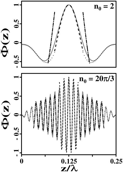
FIG. 5.: The same as Fig 3, but for scattering by a magneto-optical field. Dashed, dot-dashed and dotted lines are asymptotic dependences (120, 121, 119) respectively.

As in the case of the standing wave beam splitter, everywhere except near the points $z=0,$ $\lambda/8,$ $\lambda/4,$ the profile is a grating having a spatially inhomogeneous period

$$d\left(z\right)=d_{i}\left/\cos\left[\frac{1}{6}\left(4kz-\pi\right)\right]\right..$$ (122)

The profile is not that of an ideal beam splitter.

C Bichromatic beam splitter

Lacking an analytical expression for the potential produced by a bichromatic field we are not able to obtain an analytical asymptotic expression for the grating profile. On the other hand, it is possible to evaluate Eqs. (90) numerically. In Fig. 6 the profile is shown for $n_{0}=20\pi/3$ and is similar to that for the magneto-optical potential.

FIG. 6.: Density profile produced by bichromatic field for $n_{0}=20\pi/3.$

IV Discussion

Asymptotic expressions in the limit of large-angle scattering have been obtained for the atomic wave function and grating profile after scattering from a periodic triangular potential (see Appendix) and from potentials which approximate this triangular potential. The potentials are chosen [13, 25] with the goal of producing two and only two final state momenta

$$p=\pm 2n_{0}\hbar k,$$ (123)

with $\left(n_{0}\gg 1\right).$ In turn, interference between these momenta components in the Fresnel scattering region lead to a pure, sinusoidal high-order grating

$$\rho\left(z\right)=1+\cos\left(4n_{0}kz\right)$$ (124)

having period

$$d_{i}=\lambda/4n_{0}.$$ (125)

In practice, it is impossible to produce only two final state momenta with periodic potentials. At best, one finds scattering into two groups of states centered around $p=\pm 2n_{0}\hbar k$. Owing to the range of momenta in each group, none of the potentials can generate the ideal grating profile (124). For the potentials considered in this work, the width of the momentum groups scales asymptotically as $n_{0}^{1/3}$ [see Eqs. (38, 59, 78)]. If one’s goal is to creates a higher order sinusoidal grating, then one needs to increase the angle of splitting, i. e. the parameter $n_{0}.$ However, by increasing $n_{0}$ one broadens the width of the momentum groups, and diminishes degree to which the grating profile approximates a pure sinusoidal grating.

In the limit of strong fields and large scattering angles, we developed asymptotic techniques for evaluating the atomic wave function and density. One might think that a quasiclassical or WKB method could be used in this limit, but the linear nature of the potential invalidates such an approach in the region of maximum scattering. Instead, the method of stationary phase was used to obtain asymptotic expressions for the wave function. The results depend solely on the first and third derivatives of the potential at the point of maximum slope. For all but the triangular potential, however, these asymptotic expressions cannot be used in the expressions for the atomic density since they do not produce a convergent result.

Only for the triangular potential does the asymptotic expression for the Fourier amplitudes converge rapidly enough as a function of Fourier index $n$ to allow one to calculate the atomic density using these asymptotic formulas. The periodic triangular potential is analyzed in the Appendix. The scattered signal is a periodic function of time with period $t_{0}=T/2n_{0}$, where $T=2\pi/\omega_{2k}$ is the Talbot time (recall that time $t$ is related to the distance $x$ following the atom-field interaction zone by $t=x/u$, where $u$ is the longitudinal velocity). In a given scattering plane following the atom-field interaction, the atom density consists of three distinct spatial regions, one of the form (124) but with twice as large an amplitude, one with $\rho\left(z\right)=1,$ and one with $\rho\left(z\right)=0$. Examples of these profiles are shown in Fig. 7 in the Appendix.

For the standing wave, magneto-optical, and bichromatic field potentials, the atomic density was calculated for scattering distances $x\gg Tu^{2}/\Delta u$ [40], where $\Delta u\ll u$ is the range of longitudinal velocities[38]. The density is a periodic function of $z$ having period $\lambda/4.$

For the standing wave potential one can distinguish regions about $z=n\lambda/4$ ($n$ is an arbitrary integer) of extent $\lambda/n_{0}$ where the density has a sharp maximum [see Eq. (97)] of order unity. With the exception of these regions the density is an oscillating function of $z$ with amplitude of order $n_{0}^{-1/2}$ and spatially inhomogeneous period (100). The period becomes infinite at $z=$ $\left(n+\frac{1}{2}\right)\frac{\lambda}{4},$ which implies that, near these points, the profile is flat. All these features are seen in Fig. 3, where the grating profile is plotted for $n_{0}=2$ and $n_{0}=20\pi/3.$ The last case corresponds to the value chosen in [15] for numerical calculations. It is surprising that the analysis of the scattering in terms of two distinct spatial intervals seems to be valid even for $n_{0}=2,$ when the condition $n_{0}\gg 1$ is not satisfied.

For the magneto-optical case one has to distinguish three regions

$$\text{I }\left|z-\left(n+\frac{1}{2}\right)\frac{\lambda}{4}\right|\lesssim\lambda/n_{0,}$$

III. other values of

(126)

In region I the modulated component of the grating profile $\Phi(z)$ is described by the function $J\left[\frac{4}{3}k\theta\left(\frac{\lambda}{8}-z\right)\right]$ [see Eqs. (120, 110)]; in region I this function is of order unity and oscillates with a slowly decaying amplitude (see Fig. 2). In region II the grating profile oscillates with an amplitude of order $n_{0}^{-1}$. In the remaining region III, which accounts for most of the range when $n_{0}\gg 1$, the grating profile is similar to that found for the standing wave potential, i. e. it is a grating having amplitude of order $n_{0}^{-1/2}$ and a spatially inhomogeneous amplitude period given by Eq. (122). In contrast to the standing wave case, this period cannot be larger than $2\times 3^{-1/2}d_{i}.$ The grating profile produced by the magneto-optical field is shown in the Fig. 4. For a moderate value $n_{0}=2,$ the dependence (121) associated with region III is a poor approximation to the profile; however, one can see from Fig. 4 that it is not necessary to use the expression for region III. Regions I and II overlap with region III and with each other, and Eqs. (120, 119) provide a good approximation to the profile for all $z.$

The grating profile for the bichromatic potential is shown in Fig. 6 for $n_{0}=20\pi/3.$

In summary, we have asymptotic expressions for the momentum distribution and calculated the grating profile for several classes of optical beam splitters. While the momentum distribution resulting from these beam splitters can approach that of an ideal beam splitter, the associated grating profiles do not closely approximate a pure sinusoidal pattern.

A Appendix - Triangular Potential.

It is instructive to consider scattering by the ideal periodic triangular potential (13). This potential differs from those considered in the text in that the second derivative in each half-period of the potential vanishes identically. The pulse area associated with this potential is given by

$$\theta\left(z\right)=2kn_{0}\left\{\begin{tabular}[]{l}-$z,$ for $\left|z\right|<\lambda/8$\\ $z-\lambda/4,$ for $\left|z-\lambda/4\right|<\lambda/8$\end{tabular}\right.,$$ (A1)

where $n_{0}=\bar{n}/2.$  For the Fourier components (25), one finds

$$\psi_{n}=\left\{\begin{tabular}[]{l}$2n_{0}\sin\left[\left(n-n_{0}\right)\pi/2\right]\left/\pi\left(n^{2}-n_{0}^{2}\right)\right.,$ for $n\neq-n_{0}$\\ $\left(-1\right)^{n_{0}}/2,$ for $n=-n_{0}$\end{tabular}\right..$$ (A2)

Consider now the case of large integer $n_{0}.$ For $n$ close to $\pm n_{0}$ one finds

$$\psi_{n_{0}+\Delta n} \approx \sin\left[\Delta n\pi/2\right]\left/\pi\Delta n\right.,$$ (A4)

$$\psi_{-n_{0}+\Delta n} \approx (-1)^{n_{0}}\left[\delta\left(\Delta n\right)-\psi_{n_{0}+\Delta n}\right].$$ (A5)

where $\delta\left(\Delta n\right)$ is a Kronecker symbol.  In a contrast to the nonlinear potentials considered above, the amplitudes (A) decay sufficiently fast to calculate both the atomic wave function and atom density. In the expression for the wave function,

$$\psi\left(z,t\right) = \psi_{+}\left(z,t\right)+\psi_{-}\left(z,t\right),$$ (A7)

$$\psi_{\pm}\left(z,t\right) = \sum_{\Delta n}\psi_{\pm n_{0}+\Delta n}\exp\left[2ikz\left(\pm n_{0}+\Delta n\right)-i\omega_{2k}\left(\pm n_{0}+\Delta n\right)^{2}t\right]$$ (A8)

one can neglect terms quadratic in $\Delta n$ in the exponents if $\left|t-mT\right|\ll T$, where $m$ is an integer and $T=2\pi/\omega_{2k}$ is the Talbot time. For these values of $t$, one can obtain analytic asymptotic expressions for the wave function and density. The wave function is a periodic function of $z$ having period $\lambda/2$ and a periodic function of $t$ having a reduced Talbot period

$$t_{0}=\pi/\omega_{2k}n_{0}.$$ (A9)

Within one period

$$\psi_{+}\left(z,t\right) = \exp\left(2in_{0}kz-i\omega_{2kn_{0}}t\right)\Theta\left(\frac{\lambda}{8}-\left|z-2n_{0}\frac{\hbar k}{m}t\right|\right),$$ (A11)

$$\psi_{-}\left(z,t\right) = \exp\left(-2in_{0}kz-i\omega_{2kn_{0}}t\right)\Theta\left(\left|z+2n_{0}\frac{\hbar k}{m}t\right|-\frac{\lambda}{8}\right),$$ (A12)

where $\Theta\left(x\right)$ is a Heaviside step-function.

One sees that after scattering the wave function splits in two components having average momentum $\pm 2n_{0}\hbar k.$ Moreover, there is a spatial modulation of the wave function corresponding to $\frac{\lambda}{4}$ sections of the incident plane wave scattered with momenta $\pm 2n_{0}\frac{\hbar k}{m}$. These wave function components, having unit amplitude and spatial width $\frac{\lambda}{4}$, are centered at $z=z_{\pm},$ where

$$z_{+} = 2n_{0}\frac{\hbar k}{m}t+n_{+}\frac{\lambda}{2},$$ (A14)

$$z_{-} = -2n_{0}\frac{\hbar k}{m}t+\left(n_{-}+\frac{1}{2}\right)\frac{\lambda}{2}$$ (A15)

($n_{\pm}$ are arbitrary integers). Interference occurs when different components centered at $z_{\pm}$ overlap. Outside of the interference regions, the density can equal unity for points belonging to one of the $z_{\pm}$-regions or $0$ for other points. Analyzing all these possibilities, one arrives at the following density profile

$$\rho\left(z,t\right) = \xi\left(z,t\right)+2\left(-1\right)^{n_{0}}\cos\left(4n_{0}kz\right)\phi\left(z,t\right),$$ (A17)

$$\phi\left(z,t\right) = \left\{\begin{array}[]{ll}1&\begin{array}[]{l}\text{if }z\in\left[-\frac{3\lambda}{8}-z_{t},\frac{\lambda}{8}+z_{t}\right]\text{ and }t\in\left[-\frac{t_{0}}{2},-\frac{t_{0}}{4}\right]\\ \text{if }z\in\left[-\frac{\lambda}{8}+z_{t},-\frac{\lambda}{8}-z_{t}\right]\text{ and }t\in\left[-\frac{t_{0}}{4},0\right]\\ \text{if }z\in\left[\frac{\lambda}{8}-z_{t},\frac{\lambda}{8}+z_{t}\right]\text{ and }t\in\left[0,\frac{t_{0}}{4}\right]\\ \text{if }z\in\left[-\frac{\lambda}{8}+z_{t},\frac{3\lambda}{8}-z_{t}\right]\text{ and }t\in\left[\frac{t_{0}}{4},\frac{t_{0}}{2}\right]\end{array}\\ 0&\text{in other cases}\end{array}\right.;$$ (A24)

$$\xi\left(z,t\right) = \left\{\begin{array}[]{l}0,\text{ if }z\in\left[-\frac{\lambda}{8}-z_{t},\frac{3\lambda}{8}+z_{t}\right]\\ 1,\text{ if }z\in\left[-\frac{\lambda}{4},-\frac{3\lambda}{8}-z_{t}\right]\cup\left[\frac{\lambda}{8}+z_{t},-\frac{\lambda}{8}-z_{t}\right]\cup\left[\frac{3\lambda}{8}+z_{t},\frac{\lambda}{4}\right]\\ 2,\text{ if }z\in\left[-\frac{3\lambda}{8}-z_{t},\frac{\lambda}{8}+z_{t}\right]\end{array}\right\},\text{ for }t\in\left[-\frac{t_{0}}{2},-\frac{t_{0}}{4}\right];$$ (A28)

$$= \left\{\begin{array}[]{l}0,\text{ if }z\in\left[\frac{\lambda}{8}+z_{t},\frac{\lambda}{8}-z_{t}\right]\\ 1,\text{ if }z\in\left[-\frac{\lambda}{4},-\frac{\lambda}{8}+z_{t}\right]\cup\left[-\frac{\lambda}{8}-z_{t},\frac{\lambda}{8}+z_{t}\right]\cup\left[\frac{\lambda}{8}-z_{t},\frac{\lambda}{4}\right]\\ 2,\text{ if }z\in\left[-\frac{\lambda}{8}+z_{t},-\frac{\lambda}{8}-z_{t}\right]\end{array}\right\},\text{ for }t\in\left[-\frac{t_{0}}{4},0\right];$$ (A32)

$$= \left\{\begin{array}[]{l}0,\text{ if }z\in\left[-\frac{\lambda}{8}-z_{t},-\frac{\lambda}{8}+z_{t}\right]\\ 1,\text{ if }z\in\left[-\frac{\lambda}{4},-\frac{\lambda}{8}-z_{t}\right]\cup\left[-\frac{\lambda}{8}+z_{t},\frac{\lambda}{8}-z_{t}\right]\cup\left[\frac{\lambda}{8}+z_{t},\frac{\lambda}{4}\right]\\ 2,\text{ if }z\in\left[\frac{\lambda}{8}-z_{t},\frac{\lambda}{8}+z_{t}\right]\end{array}\right\},\text{ for }t\in\left[0,\frac{t_{0}}{4}\right];$$ (A36)

$$= \left\{\begin{array}[]{l}0,\text{ if }z\in\left[-\frac{3\lambda}{8}+z_{t},\frac{\lambda}{8}-z_{t}\right]\\ 1,\text{ if }z\in\left[-\frac{\lambda}{4},-\frac{3\lambda}{8}+z_{t}\right]\cup\left[\frac{\lambda}{8}-z_{t},-\frac{\lambda}{8}+z_{t}\right]\cup\left[\frac{3\lambda}{8}-z_{t},\frac{\lambda}{4}\right]\\ 2,\text{ if }z\in\left[-\frac{\lambda}{8}+z_{t},\frac{3\lambda}{8}-z_{t}\right]\end{array}\right\},\text{ for }t\in\left[\frac{t_{0}}{4},\frac{t_{0}}{2}\right];$$ (A40)

where

$\displaystyle z_{t}=\frac{\lambda t}{2t_{0}}.$

This profile is shown in Fig. 7. The function $\phi\left(z,t\right)$ represents an envelope function for higher order gratings having period $d_{i}=\lambda/4n_{0}.$

FIG. 7.: Scattering by the triangular potential. The first seven graphs give the density profile for a single period at different times. The last graph if the density averaged over $t_{0}$. The time $t_{0}$ is the Talbot time divided by $n_{0}$ and $n_{0}=11$ in this figure.

Expression (A24) gives the envelope at a given time. One can consider also the grating profile as a function of $t$ for given $z$. This would correspond to atoms arriving at a given $z$ with different longitudinal velocities, allowing one to make a comparison with the results of Sec. III. For fixed $z$ as a function of $t$, one finds

$$\phi\left(z,t\right)=\left\{\begin{array}[]{ll}1&\begin{array}[]{l}\text{if }t\in\left[-\frac{3}{4}t_{0}-2\frac{z}{\lambda}t_{0},\frac{1}{4}t_{0}+2\frac{z}{\lambda}t_{0}\right]\text{ and }z\in\left[-\frac{\lambda}{4},-\frac{\lambda}{8}\right]\\ \text{if }t\in\left[-\frac{1}{4}t_{0}+2\frac{z}{\lambda}t_{0},-\frac{1}{4}t_{0}-2\frac{z}{\lambda}t_{0}\right]\text{ and }z\in\left[-\frac{\lambda}{8},0\right]\\ \text{if }t\in\left[\frac{1}{4}t_{0}-2\frac{z}{\lambda}t_{0},\frac{1}{4}t_{0}+2\frac{z}{\lambda}t_{0}\right]\text{ and }z\in\left[0,\frac{\lambda}{8}\right]\\ \text{if }t\in\left[-\frac{1}{4}t_{0}+2\frac{z}{\lambda}t_{0},\frac{3}{4}t_{0}-2\frac{z}{\lambda}t_{0}\right]\text{ and }z\in\left[\frac{\lambda}{8},\frac{\lambda}{4}\right]\end{array}\\ 0&\text{in other cases}\end{array}\right.$$ (A41)

One sees that over one period of Talbot oscillations the high harmonic amplitude is constant for some times and vanishes for others. The harmonic amplitude averaged over a Talbot oscillation period is simply given by $\left\langle\phi\left(z,t\right)\right\rangle_{t}=t_{z}/t_{0},$ where $t_{z}$ is the duration of the time interval when the harmonic amplitude is constant; the background term on average is equal to unity $\left[\left\langle\xi\left(z,t\right)\right\rangle_{t}=1\right].$ Calculating $t_{z}$ from A41, one finds

$$\left\langle\rho\left(z,t\right)\right\rangle_{t} = 1+2\left(-1\right)^{n_{0}}\cos\left(4n_{0}kz\right)$$ (A45)

$$\times\left\{\begin{array}[]{l}1-\frac{4}{\lambda}\left|z\right|,\text{ for }\left|z\right|>\frac{\lambda}{8}\\ \frac{4}{\lambda}\left|z\right|,\text{ for }\left|z\right|<\frac{\lambda}{8}\end{array}\right\}.$$

This result could be obtained using Eqs. (III, III) of Sec. III with the pulse area (A1).

REFERENCES

• [1] B. Dubetsky, A. P. Kazantsev, V. P. Chebotayev, V. P. Yakovlev, Pis’ma Zh. Eksp. Teor. Fiz. 39, 531 (1984) [JETP Lett. 39, 649 (1985)].
• [2] A. P. Kazantsev, G. I. Surdutovich, V. P. Yakovlev, Pis’ma Zh. Eksp. Teor. Fiz. 31, 542 (1980) [JETP Lett. 31, 509 (1980)].
• [3] P. E. Moskowitz, P. L.Gould, S. R. Atlas, and D. E. Pritchard, Phys. Rev. Lett. 51,370,1983.
• [4] E. M. Rasel, M. K. Oberthaler, H. Batelaan, J. Schmiedmayer, A. Zeilinger, Phys. Rev. Lett. 75, 2633 (1995).
• [5] M. Prentiss, G. Timp, N. Bigelow, R. E. Behringer, J. E. Cunningham, Appl. Phys. Lett. 60, 1027, (1992).
• [6] T. Sleator, T. Pfau, V. Balykin, J. Mlynek, Appl. Phys. B 54, 375, (1992).
• [7] B. Dubetsky and P. R. Berman, Phys. Rev. A 50, 4057 (1994).
• [8] P. R. Berman, B. Dubetsky, and J. L. Cohen, Phys. Rev. A 58, 4801 (1998).
• [9] D. M. Giltner, R. W. McGowan, S. A. Lee, Phys. Rev. Lett. 75, 2638 (1995).
• [10] J. L. Cohen, Thesis, University of Michigan, 2000, pp. 140-143.
• [11] A. V. Turlapov, D. V. Strekalov, A. Kumarakrishnan, S. Cahn, and T. Sleator, in ICONO 98: Quantum Optics, Interference Phenomena in Atomic Systems, and High-Precision Measurements (edited by A. V. Andreev, S. N. Bagayev, A. S. Chirkin, and V. I. Denisov), SPIE Proc. 3736, 26-37 (1999).
• [12] P. R. Berman and B. Bian, Phys. Rev. A 55, 4382 (1997).
• [13] R. Grimm, V. S. Letokhov, Yu. B. Ovchinnikov, A. I. Sidorov, J. Phys. II France, 2, 593 (1992).
• [14] T. Pfau, Ch. Kurtsiefer, C. S. Adams, M. Sigel, J. Mlynek, Phys. Rev. Lett. 71, 3427 (1993).
• [15] C. S. Adams, T. Pfau, Ch. Kurtsiefer, J. Mlynek, Phys. Rev. A, 48, 2108 (1993).
• [16] U. Janicke, M. Wilkens, Phys. Rev. A, 50, 3265 (1994).
• [17] A. P. Chu, K. S. Johnson, and M. G. Prentiss, J. Opt. Soc. Am. B 13, 1352 (1996).
• [18] J. Soding, R. Grimm, Phys. Rev. A, 50, 2517 (1994).
• [19] K. S. Johnson, A. Chu, T. W. Lynn, K. K. Berggren, M. S. Shahriar, and M. Prentiss, Opt. Lett. 20, 1310 (1995).
• [20] V. S. Voitsekhovich, M. V. Danileiko, A. M. Negriiko, V. I. Romanenko, and L. P. Yatsenko, Zh. Tekh. Fiz. 58, 1174 (1988) [Sov. Phys. Tech. Phys. 33, 690 (1988)].
• [21] V. S. Voitsekhovich, M. V. Danileiko, A. M. Negriiko, V. I Romanenko, and L. P. Yatsenko, Pis’ma Zh. Eksp.Teor. Fiz. 49, 138 (1989) [JETP Lett. 49, 161 (1989)].
• [22] R. Grimm, Yu. B. Ovchinnikov, A. I. Sidorov, V. S. Letokhov, Phys. Rev. Lett. 65, 1415 (1990);
• [23] J. Soding, R. Grimm, Yu. B. Ovchinnikov, P. Bouyer, and Ch. Salomon, Phys. Rev. Lett. 78, 1420 (1997).
• [24] M. Williams, F. Chi, M. Cashen, and H. Metcalf, Phys. Rev. A 61, 023408 (2000).
• [25] R. Grimm, J. Soding, Yu. B. Ovchinnikov, Opt. Lett. 19, 658 (1994).
• [26] K. S. Johnson, A. P. Chu, K. K. Berggren, and M. G. Prentiss, Optics Comm. 126, 326 (1996).
• [27] S. M. Tan, D. F. Walls, Opt. Commun. 118, 412 (1995).
• [28] T. Wong, M. K. Olsen, S. M. Tan, D. F. Walls, Phys. Rev. A 52, 2161 (1995).
• [29] E A Korsunsky, Yu. B. Ovchinnikov, Optics Comm. 143, 219 (1997).
• [30] A. S. Pazgalev and Yu. V. Rozhdestvenski, Pisma Zh. Eksp. Teor. Fiz. 66, 386 (1997) [JETP Lett., 66, 412 (1997)].
• [31] E. A. Korsunsky, Quantum Semiclass. Opt. 10, 477 (1998).
• [32] V. I. Romanenko and L. P. Yatsenko, Zh. Eksp. Teor. Fiz. 117, 467 (2000).[JETP 90, 407 (2000)].
• [33] P. R. Berman, Phys. Rev. A 53, 2627 (1996).
• [34] P. L. Gould, D. E. Pritchard, In Proceedings of the International School of Physics ”Enrico Fermi”, Course CXXXI, edited by A. Aspect, W. Barletta and R. Bonifacio (Amsterdam, Oxford, Tokio, Washington DC) 1996, p. 443.
• [35] M. Abramowitz and I. A. Stegun editors, ”Handbook of Mathematical Functions,” Dover Publications, Inc. (New York, 1972), p. 366, No. 9.3.4.
• [36] J. L. Cohen, B. Dubetsky, and P. R. Berman, Phys. Rev. A 60, 4886 (1999).
• [37] The distance $x$ is always confined to the Fresnel scattering zone, which for a beam of diameter $b$ requires $x\phi\ll b,$ where $\phi\sim n_{0}\hbar k/Mu$ is the scattering angle.
• [38] B. Dubetsky and P. R. Berman, In ”Atom Interferometry”, edited by P. R. Berman (Academic Press, Cambridge, MA, 1997), p 407 (or http://arXiv.org/PS_cache/physics/pdf/0005/0005078. pdf), Sec. VI.
• [39] N. Guerineau, B. Harchaoui, and J. Primot, Opt. Commun. 180, 199 (2000).
• [40] This condition could be too strong. For example in the triangular potential the averaged profile arises for distances $x\gg t_{0}u^{2}/\Delta u$ , which are $2n_{0}$ times smaller than those given by Eq. (82).