A MULTISECTION BROADBAND IMPEDANCE TRANSFORMING BRANCH-LINE HYBRID

Abstract

Measurements and design equations for a two section impedance transforming hybrid suitable for MMIC applications and a new method of synthesis for multisection branch-line hybrids are reported. The synthesis method allows the response to be specified either of Butterworth or Chebyshev type. Both symmetric (with equal input and output impedances) and non-symmetric (impedance transforming) designs are feasible. Starting from a given number of sections, type of response, and impedance transformation ratio and for a specified midband coupling, power division ratio, isolation or directivity ripple bandwidth, the set of constants needed for the evaluation of the reflection coefficient response is first calculated. The latter is used to define a driving point impedance of the circuit, synthesize it and obtain the branch line immittances with the use of the concept of double length unit elements (DLUE). The experimental results obtained with microstrip hybrids constructed to test the validity of the brute force optimization and the synthesized designs show very close agreement with the computed responses.

Keywords: Microwave circuits, distributed parameter synthesis, Butterworth and Chebyshev filters.

I Introduction

Branch line hybrids are extensively used in the realization of a variety of microwave circuits. Balanced mixers, data modulators, phase shifters, and power combined amplifiers are some examples of such circuits. Single section hybrids have a limited bandwidth. For example, a single section quad hybrid with equal power division has a bandwidth of about $15\%$ over which the power balance is within 0.5 dB. It is well known that the operating bandwidth can be greatly increased using multisection hybrids. Most applications require also that the $50\Omega$ input impedance be transformed to a higher or lower impedance. A hybrid with built-in impedance transformation is limited by the practical realizability of the line impedances of the various branches.

Although a higher bandwidth may be achieved using a coupled line configuration instead of a branch line one, coupled line hybrids are difficult to realize, particularly if microwave monolithic integrated circuits (MMIC) implementation is used. The branch line hybrid has the advantage that it may be realized using slot lines in the ground plane of a microstrip circuit. In this case the hybrid requires virtually no additional real estate on the chip. This may be an important consideration when the hybrid is part of a larger MMIC circuit. At lower microwave frequencies (5 GHz or less) a lumped element realization similar to that of [1] may be used to implement an MMIC hybrid.

For some applications it may be sufficient to employ a two section impedance transforming hybrid which has ideal performance at the center of the desired frequency band. Design equations for such a hybrid are derived in the next section. A general synthesis method for multisection hybrids is also reported. The hybrid is in effect a four port impedance transforming structure. Synthesis procedures for two port impedance transformers using quarter wave sections to realize a Butterworth or Chebyshev type response are well known. The synthesis method reported here, similar to that used by Levy and Lind [6], is applied to the hybrid with only the two port even mode circuit being synthesized. There are however, important differences from [6] which are brought out in the section on synthesis. This paper is organized as follows: In section II we describe and analyze the performance of the two-section broadband hybrid and in section III a general method for the synthesis of multisection hybrids is described. Section IV contains a comparative discussion between the measurements, optimization and synthesis and contains our conclusions.

II ANALYSIS AND PERFORMANCE OF THE TWO-SECTION HYBRID

A two-section branch-line quadrature hybrid is shown in Figure 1. Using odd-even mode analysis, the even and odd mode cascade element matrices at the center frequency are given by:

$$M_{e}=\left[\begin{array}[]{ c c}A&B\\ C&D\end{array}\right]\mbox{; }M_{o}=\left[\begin{array}[]{ c c}A&-B\\ -C&D\end{array}\right]$$ (5)

where:

$$A=\frac{b^{2}}{cd}-1;B=-j\frac{b^{2}}{c};C=-j(\frac{1}{a}+\frac{1}{d}-\frac{b^{2}}{acd})$$

$$\hskip 56.9055pt\mbox{ and }D=\frac{b^{2}}{ac}-1$$ (6)

Use of the relation between cascade parameters and the reflection and transmission coefficients [3] and application of matching and perfect isolation conditions ($S_{11}=0$ and $S_{41}=0$ at the center frequency) results in:

$$A=DZ_{01}/Z_{02},B=CZ_{01}Z_{02}$$ (7)

where $Z_{01},Z_{02}$ are input (ports 1 and 4) and output (ports 2 and 3) impedances respectively.

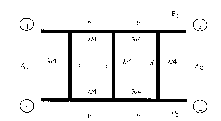
Figure 1: Two-section branch line impedance transforming hybrid $a,b,c,d$ are the characteristic impedances of the quarter wave branches.

The normalized voltage waves $b_{2}$ and $b_{3}$ at the output ports are given in terms of the odd and even mode transmission coefficient. $T_{e}\mbox{ and }T_{o}$ by $b_{2}=(T_{e}+T_{o})/2$ and $b_{3}=(T_{e}-T_{o})/2$. Once again using the relation between the transmission coefficients and the cascade parameters [3] the output port power ratio may be written as:

$$\frac{P_{3}}{P_{2}}=\frac{P_{out}\mbox{ at }port3}{P_{out}\mbox{ at }port2}=k^{2}$$ (8)

with:

$$k=|\frac{b_{3}}{b_{2}}|=|\frac{C}{A}Z_{01}|$$ (9)

This gives:

$$C^{2}=-k^{2}A^{2}/{Z_{01}}^{2}$$ (10)

The negative sign was retained in (5) as equation (1) implies $C^{2}$ to be a negative quantity. A relation between the line impedances a and d is found by first solving for $b^{2}/c$ using (1), the two components of (2) and then equating the two values of $b^{2}/c$ thus found. This gives:

$$\frac{1}{a^{2}}=\frac{r}{d^{2}}+\frac{(1-r)}{r{Z_{01}}^{2}}$$ (11)

where $r$, the impedance transformation ratio is defined by the ratio $Z_{01}/Z_{02}$. In order to obtain design equations for the line impedances $a,d$ another equation relating these impedances is needed. This is obtained by applying the losslessness condition: $|b_{2}|^{2}+|b_{3}|^{2}=1$ along with (3):

$$|b_{2}|^{2}=1/(1+k^{2})$$ (12)

Substitution for $b_{2}$ in terms of $T_{e}\mbox{ and }T_{o}$ and use of (1) and (5) result in:

$$b_{2}=\frac{1}{A\sqrt{r}(1+k^{2})}$$ (13)

From (7) and (8):

$$A=-\frac{1}{\sqrt{r(1+k^{2})}}$$ (14)

The negative sign was retained in equation (9) as this solution gives non negative values of the branch impedances. Using (9) and relations between the cascade parameters and line impedances in (1) we can obtain the second equation relating $a$ and $d$ as:

$$a=d\frac{\sqrt{r(1+k^{2})}-1}{\sqrt{r(1+k^{2})}-r}$$ (15)

From [6] and [10] the line impedance $a$ is:

$$a = Z_{01}\frac{\sqrt{r(t^{2}-r)}}{t-r}\hskip 28.45274pt\mbox{ with $t$ defined as }$$

$$t = r\sqrt{1+k^{2}}$$ (16)

Substitution back gives:

$$d=Z_{01}\frac{\sqrt{r(t^{2}-r)}}{t-1}$$ (17)

and:

$$b^{2}/c=Z_{01}\sqrt{r-r^{2}/t^{2}}$$ (18)

Equations (11), (12) and (13) can be used to design the two section hybrid with a given impedance transformation ratio $r$ and the power ratio (coupling) $k^{2}$. Note that the ratio $b/c$ can be chosen to be different from 1. However, $b=c$ gives maximum bandwidth when the best performance at the band center is specified. Impedances $b$ and $c$ are commonly chosen to be equal.

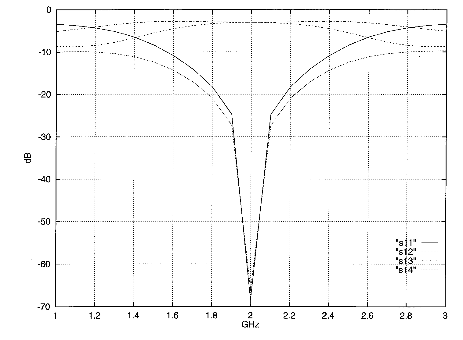
Figure 2: Computed frequency response of a two-section $50\Omega$ to $35\Omega$ hybrid. The impedance values used are $a=72.5\Omega,b=29.6\Omega,c=29.6\Omega$ and $d=191.25\Omega$.

For equal power division, $k=1$ and $t^{2}=2r^{2}$. The minimum value for $r$ for non negative branch impedances is 0.5. In practice, $r$ in the range of .7 to 1.3 for a 50$\Omega$ input impedance gives practically realizable line impedances. Referring to Fig.1, the computed line impedance values of an equal power division, 50 to 35$\Omega$ two-section hybrid are: $a=72.5\Omega$, $b=29.6\Omega$, $c=29.6\Omega$ and $d=191.25\Omega$.

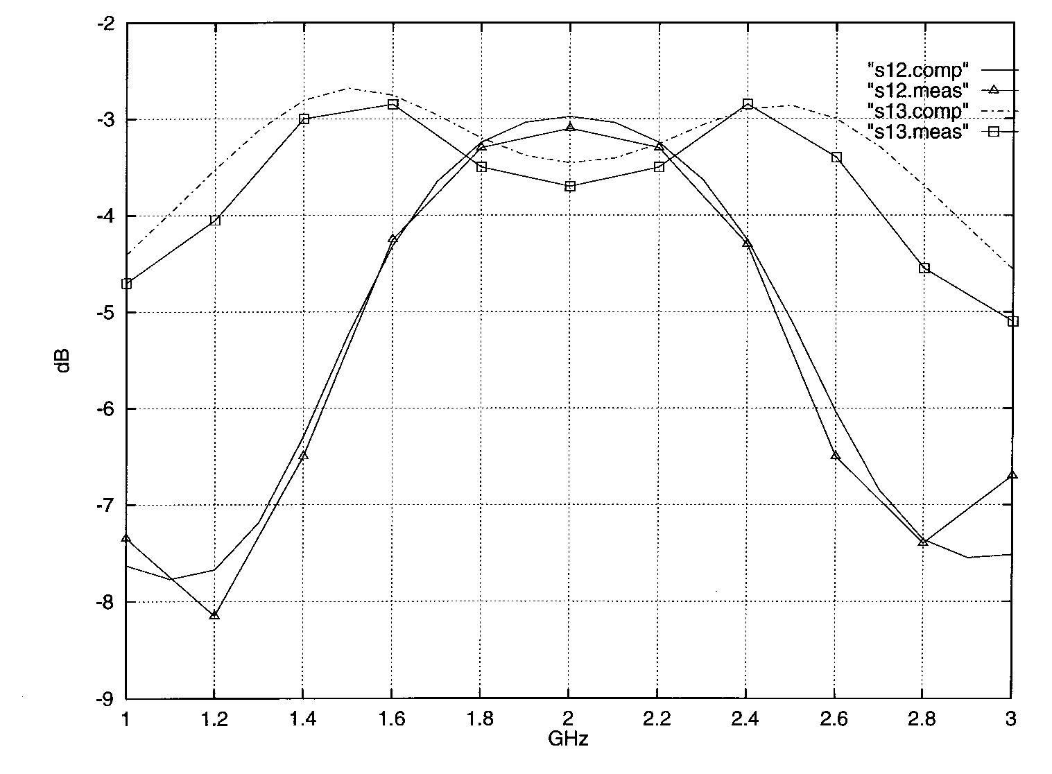
Figure 3: Computed and measured $S_{12}$ and $S_{13}$ responses for the optimized hybrid. The hybrid was fabricated on a Rogers 5880, 0.031 inch thick Duroid substrate. A wide band three- section Chebyshev transformer was used at the output ports to transform the $35\Omega$ impedance back to $50\Omega$ for the measurement. The optimized impedance values are $a=90\Omega$, $b=39\Omega$, $c=56\Omega$ and $d=110\Omega$.

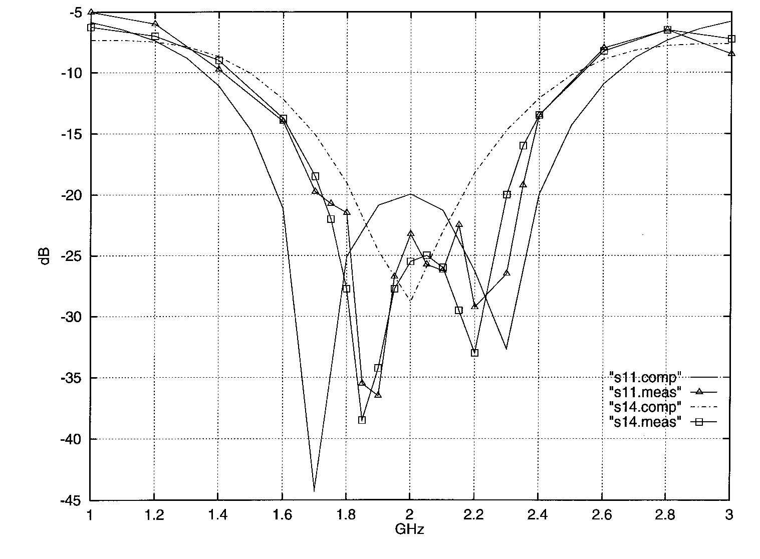
Figure 4: Computed and measured $S_{11}$ and $S_{14}$ responses for the optimized hybrid described in Fig.3.

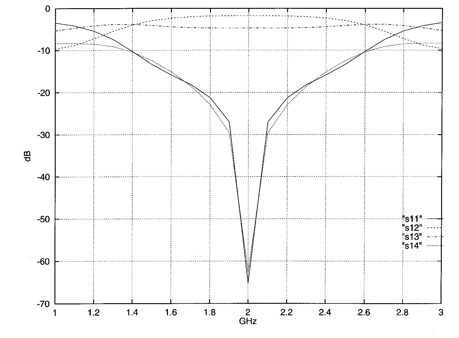
Figure 5: Computed response of a two-section $50\Omega$ to $50\Omega$ with 3 dB unequal power division hybrid. The computed values for a 3 dB unequal power division, i.e. $k=0.707$, non impedance transforming hybrid are $a=d=157\Omega,b=c=29\Omega$.

The computed frequency response for a 2 GHz hybrid is shown in Fig. 2. As may be seen from this figure, a 0.5dB output balance bandwidth of $25\%$ is feasible. However, the response can be further improved by computer optimization. In carrying out the optimization, limits were placed on the impedance values in order to yield an easily realizable design. A multisection hybrid offers the flexibility of carrying out this optimization quite effectively. The T- junction discontinuity effects can also be included in the program. Such effects become quite important at higher frequencies. Referring to Fig. 1, the optimized impedance values are: $a=90\Omega,b=39\Omega,c=56\Omega,d=110\Omega$. The hybrid was fabricated on a Rogers 5880, 0.031 inch thick Duroid substrate. A wide band three section Chebyshev transformer was used at the output ports to transform the $35\Omega$ impedance back to $50\Omega$ for the measurement. The computed and measured results for $S_{12}$ and $S_{13}$ are shown in Fig.3 while the same for $S_{11}$ and $S_{14}$ are shown in Fig.4. These results show that the agreement between the measured and computed responses is quite close and a 0.5dB balance bandwidth of $30\%$ was realized with a built-in impedance transformation from 50 to 35$\Omega$.

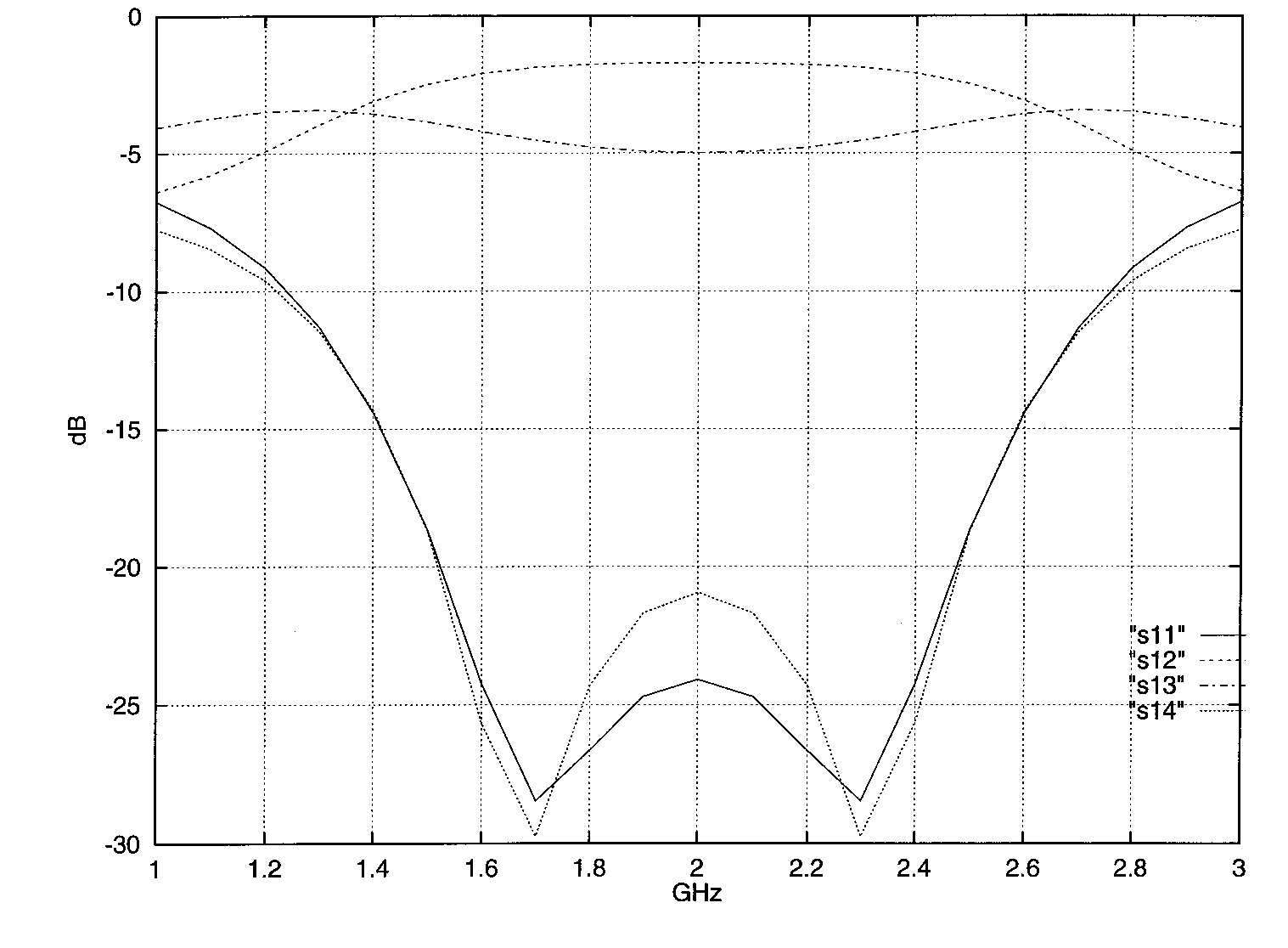
Figure 6: Computed response for the optimized 3dB unequal power division hybrid ($r=1$) The optimized impedance values are $a=135\Omega,b=46\Omega,c=92\Omega$ and $d=134\Omega$. These impedance values are suitable for slotline implementation. The computed frequency response for the optimized impedances has a wider bandwidth.

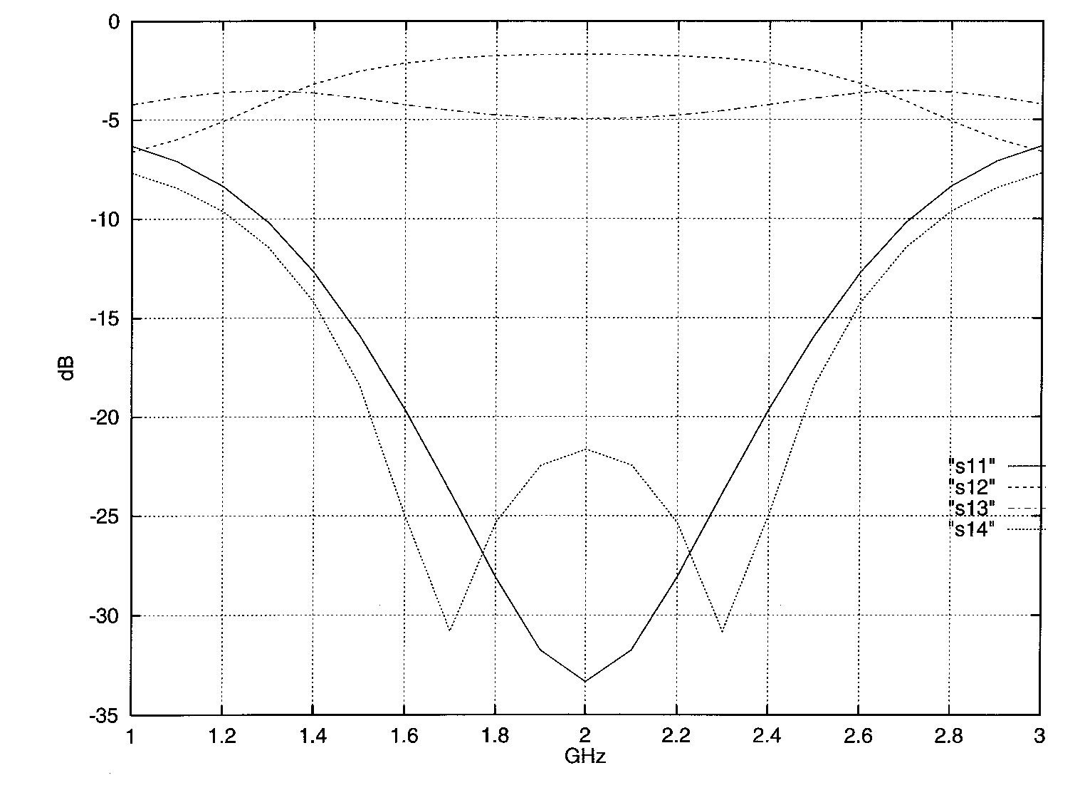
Figure 7: Computed response for the optimized 3 dB unequal power division 2 GHz hybrid ($r=1.2$). The optimized branch line impedances are $a=170\Omega,b=47\Omega,c=77\Omega,d=151\Omega$. As may be seen, the 0.5 dB balance bandwidth is $30\%$ and the return loss and isolation are better than 20 dB over the bandwidth.

The computed values for a 3dB unequal power division, i.e. $k=0.707$, non impedance transforming hybrid are $a=d=157\Omega,b=c=29\Omega$. The computed frequency response for such a hybrid is shown in Fig. 5. While the return loss and isolation values in Fig. 5 are better than 20 dB over a $25\%$ bandwidth, the branch line impedances are not suitable for slotline or microstrip implementation. The circuit, however, can also be improved with computer optimization. The optimized impedance values are: $a=135\Omega,b=46\Omega,c=92\Omega,d=134\Omega$. These impedance values are suitable for slotline implementation. The computed frequency response for the optimized hybrid is shown in Fig. 6. As can be seen from this figure, the hybrid performance did not degrade as a result of optimization for realizable branch impedances. The branch line impedances for a 6 dB unequal power split $50\Omega$ to $50\Omega$ two-section hybrid did not result in practically achievable branch line impedances for either microstrip or slotline.

The optimized branch line impedances for a 2 GHz 50$\Omega$ to $60\Omega$, 3dB unequal power division hybrid are $a=170\Omega,b=47\Omega,c=77\Omega,d=151\Omega$. Fig. 7 shows the computed response of the hybrid and a 0.5dB balance bandwidth of $30\%$ with return loss and isolation better than 20 dB over this bandwidth.

As a result of computer optimization, substantial improvement was possible for both equal and unequal power division cases. This shows that a design for ideal performance at the band center is not adequate when maximum possible bandwidth is required. Moreover the design equations for an impedance transforming, unequal power division hybrid become quite complex as the number of sections increases beyond two. In the next section, we develop a general method that can handle multisection impedance transforming hybrids and perform the synthesis numerically. The starting point in this method is based on the analytical approach of [6].

III GENERAL SYNTHESIS OF A MULTISECTION BRANCH LINE HYBRID

A general multisection branch-line hybrid is shown in Figure 8. The synthesis problem of this four-port circuit is equivalent to that of synthesizing the two-port even mode circuit. Starting from a given function $\Gamma_{e}/T_{e}$ where $\Gamma_{e}$ is the even mode reflection coefficient of the circuit and $T_{e}$ the even mode transmission coefficient, one can extract a cascade of double-lengths unit elements (DLUE) and single length open circuited shunt stubs [Fig.8]. The procedure is applicable to the Butterworth as well as the Chebyshev response for $\Gamma_{e}/T_{e}$.

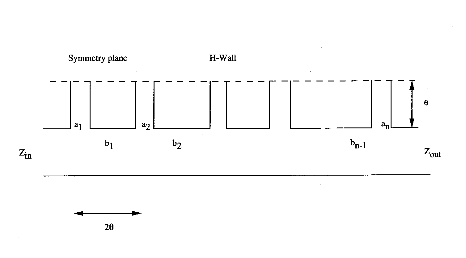
Figure 8: Even-mode circuit showing the electrical lengths and respective immittances. In comparison with Fig.1 the first immittance values are: $a_{1}=1/a,a_{2}=1/c,a_{3}=1/d,b_{1}=1/b,b_{2}=1/b$.

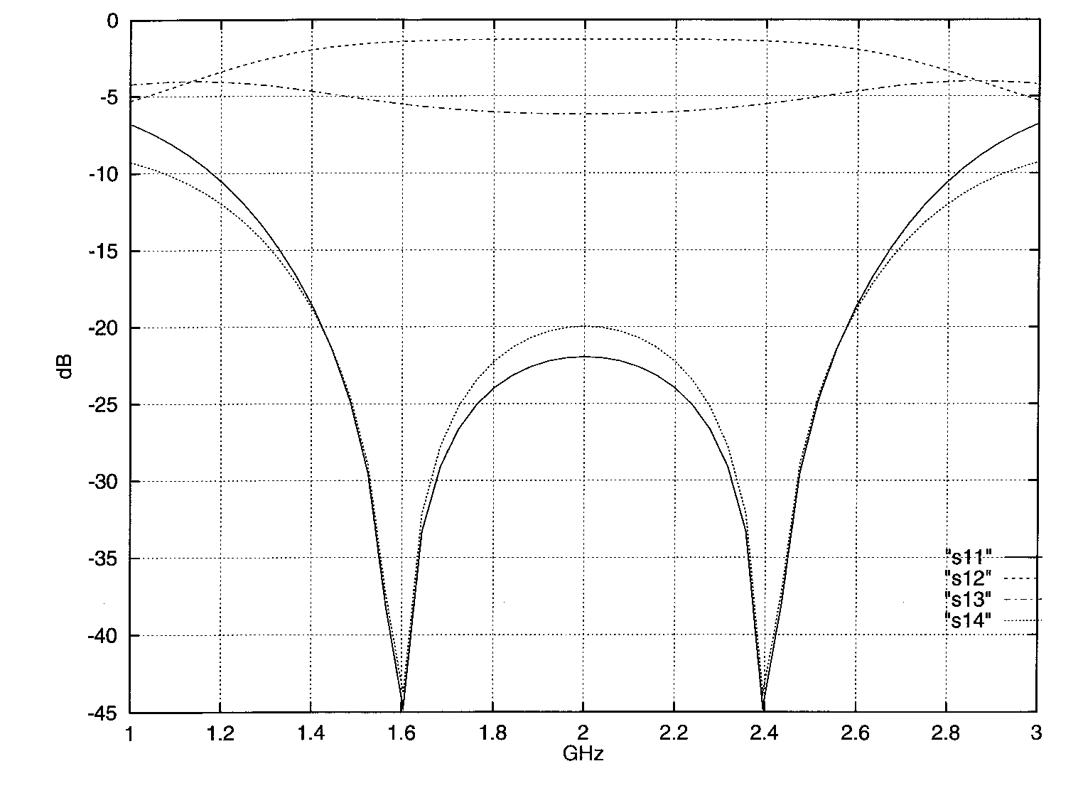
Figure 9: Computed response for the Chebyshev synthesized hybrid of Fig. 3. The hybrid is impedance transforming ($50\Omega$ to $35\Omega$) and is required to have 0 dB power division ratio at midband (2 GHz) and an isolation of -20 dB. The impedance values are: $a_{1}=157.50\Omega,a_{2}=85.05\Omega,a_{3}=99.88\Omega,b_{1}=39.49\Omega,b_{2}=33.49\Omega$.

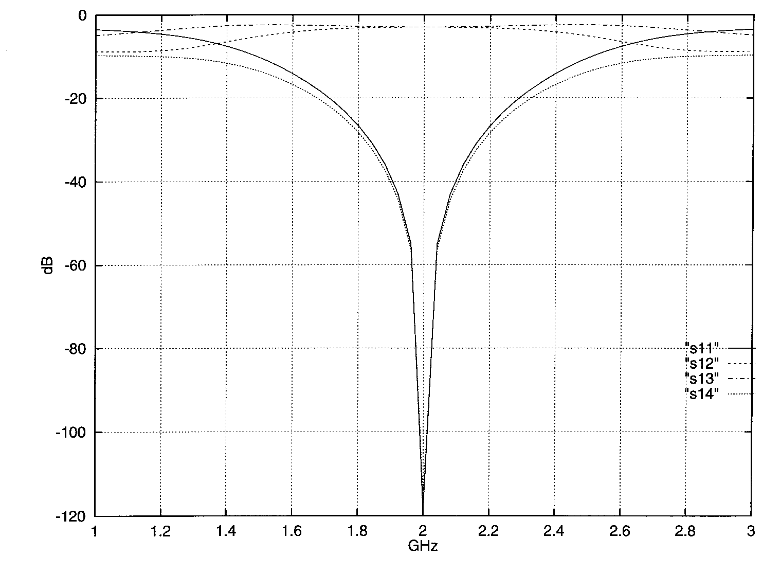
Figure 10: Computed response for the Butterworth synthesized hybrid of Fig. 3. The hybrid is impedance transforming ($50\Omega$ to $35\Omega$) and is required to have 0 dB power division ratio at midband (2 GHz). The impedance values are $a_{1}=129.20\Omega,a_{2}=31.24\Omega,a_{3}=79.37\Omega,b_{1}=33.56\Omega,b_{2}=27.55\Omega$.

A well-known synthesis method of two-port circuits is the Darlington method. In this method the response is specified and the losslessness condition: $|\Gamma_{e}|^{2}+|T_{e}|^{2}=1$ is used to extract $|\Gamma_{e}|^{2}$. The next step entails extraction of a complex function $\Gamma_{e}$ from its modulus squared. In order to do this extraction properly, the Hürwitz criterion must be respected [7]. Once $\Gamma_{e}$ is obtained, the driving point impedance of the circuit $Z_{in}=(1+\Gamma_{e})/(1-\Gamma_{e})$ can be calculated.

The extraction of the shunt stubs and the DLUE from $Z_{in}$ is done sequentially. In the symmetric case ($Z_{02}/Z_{01}=1$) the function given by Levy et al. [6] and certified by Riblet [5] was used. However, we differ in the way we adapt the Darlington synthesis to the extraction of the individual elements. For instance, the formula used to extract the first shunt stub $a_{1}$ is:

$$a_{1}=-\frac{1}{Z_{in}^{2}}{(\frac{dZ_{in}}{ds})}_{s=1}$$ (19)

where s is Richard’s variable. The DLUE is extracted by a sequential extraction of two single length unit elements (SLUE). A condition for the extraction of a SLUE is [7]:

$$Z_{in}(s=-1)=-Z_{in}(s=1)$$ (20)

After an SLUE is extracted, the driving point impedance becomes:

$$Z^{\prime}_{in}(s)=Z_{in}(1)[\frac{sZ_{in}(1)-Z_{in}(s)}{sZ_{in}(s)-Z_{in}(1)}]$$ (21)

For the sequential extraction to work it is necessary that the transformed impedance satisfies (15). Further, $Z_{in}(1)$ has to be equal to $Z^{\prime}_{in}(1)$ for the two extracted values to be same. This is a significant variation from the method used in [6]. Finally, the last shunt stub is extracted from a straight division of the denominator by the numerator of the last $Z_{in}$. In the asymmetric case, we use the function $\Gamma_{e}/T_{e}$ given in [4] and proceed exactly as in the symmetric case. In this case $Z_{02}/Z_{01}=r$ where $r\neq 1$, the function $\Gamma_{e}/T_{e}$ for an (n-1)-section hybrid is given by:

$$\frac{\Gamma_{e}}{T_{e}}=\frac{1}{\sqrt{r}}\frac{P_{n-1}(X/X_{c})}{P_{n-1}(1/X_{c})}[(r-1)-jKtg(\theta)]$$ (22)

This function depends on two parameters $X_{c}$ and $K$ that ought to be determined from the coupling $(|b_{3}|^{2})$ at the center frequency and the directivity ripple bandwidth specifications as explained below. In the Butterworth case, $X_{c}=1$ and the polynomial function $P_{n-1}(X/X_{c})$ is given by $X^{(n-1)}$ with $X=(1+s^{2})/(1-s^{2})$. Only one parameter ($K$) needs to be determined from the specification of a given value for the midband coupling (incidentally, the same procedure applies for specified midband power division ratio or isolation). The value of $K$ is numerically found as the root of the following equation:

$${[20\mbox{ log}_{10}(|T_{e}-T_{o}|/2)-|b_{3}|^{2}]}_{K}=0$$ (23)

In the Chebyshev case, the polynomial function $P_{n-1}(X/X_{c})$ is given by [6]:

$$P_{n-1}(X/X_{c})=(1+\sqrt{1-X_{c}^{2}})T_{n-1}(X/X_{c})/2-$$

$$\hskip 42.67912pt(1-\sqrt{1-X_{c}^{2}})T_{n-3}(X/X_{c})/2$$ (24)

where $T_{n}(x)$ are the generalized Chebyshev functions defined over the entire real axis. The Chebyshev case is more complex since one has to find numerically the bandwidth parameter $X_{c}$ and the parameter $K$ from the roots of the following coupled equations:

$${[20\mbox{ log}_{10}(|T_{e}-T_{o}|/2)-|b_{3}|^{2}]}_{K,X_{c}}=0$$ (25)

and:

$${[20\mbox{ log}_{10}\{|(T_{e}-T_{o})/(\Gamma_{e}-\Gamma_{o})|\}]}_{K,X_{c}}$$

$$\mbox{}-{[20\mbox{ log}_{10}\{|(T_{e}-T_{o})/(\Gamma_{e}-\Gamma_{o})|\}]}_{K,X_{2}}-20=0$$

The reference parameter $X_{2}$ corresponds to the frequency where the directivity falls by 20dB from its value at $X_{c}$. Once the parameters $X_{c}$ and $K$ have been determined from the specifications, one proceeds to the determination of the $a_{i}$’s and $b_{i}$’s. We are now in a position to make detailed comparisons with the measurements and optimization as well. The first example we tackle is the wideband two section impedance transformer ($50\Omega$ to $35\Omega$) with specified zero power division at midband. Optimization and measurements are compared for this hybrid in Figs 3 and 4 while synthesis results are shown in Figs 9 and 10. We display all the S parameters for both Butterworth and Chebyshev types of response. The resulting impedance values in the Chebyshev case are: $a_{1}=157.50\Omega,a_{2}=85.05\Omega,a_{3}=99.88\Omega,b_{1}=39.49\Omega,b_{2}=33.49\Omega$. When the specified type of response is Chebyshev, while a good isolation is obtained at midband (-20 dB), a zero power division ratio could not be obtained. This happens if a wide band, good isolation and impedance transformation ratio of 0.7 are simultaneously required. The actual power division ratio obtained is around -5 dB. When any of these conditions is relaxed the required solution exists and is shown in Fig. 10 for the Butterworth case and in Fig. 11 for the modified Chebyshev case as explained below.

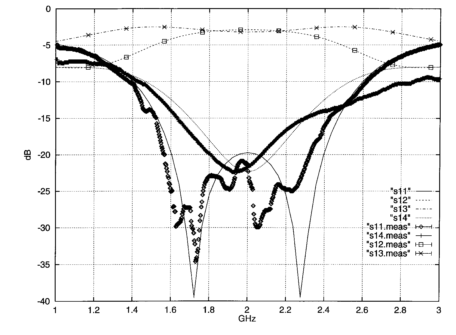
Figure 11: Computed and measured responses for the modified Chebyshev synthesized hybrid. The constants $K$ and $X_{c}$ required for the synthesis are calculated with specified 0 dB power division ratio at midband but with $r=1$. Once the synthesis is done, the S parameters are calculated from the cascaded elements using the right value for $r$ (0.7). The impedances are $a_{1}=100\Omega,a_{2}=43\Omega,a_{3}=100\Omega,b_{1}=b_{2}=35.2\Omega$. The isolation obtained at midband is about -22.5 dB.

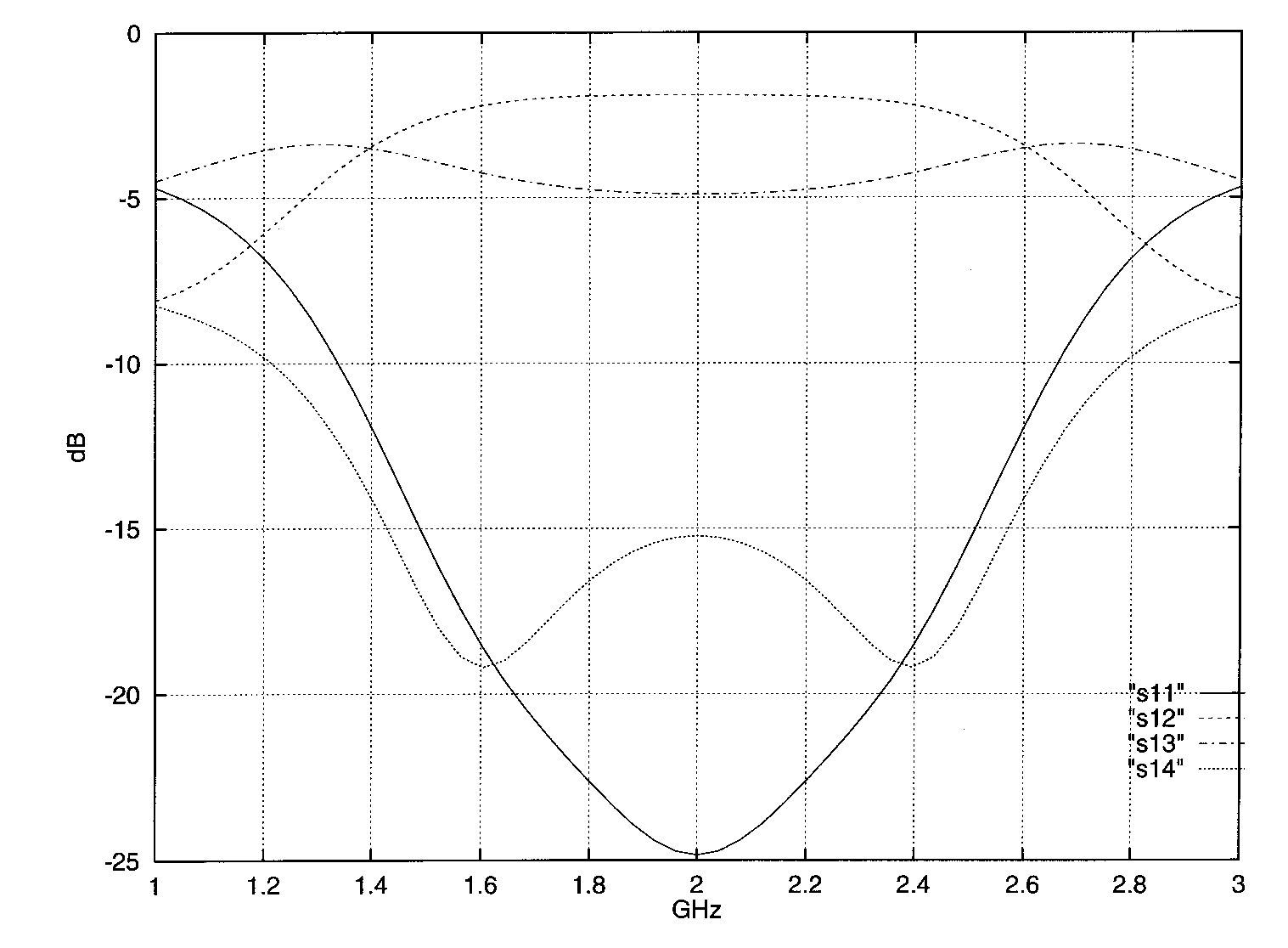
Figure 12: Computed response for the Chebyshev synthesized 3 dB unequal power division 2 GHz hybrid ($r=1.2$) corresponding to Fig. 7. The obtained isolation at midband is about -15 dB. The impedance values are $a_{1}=161.31\Omega,a_{2}=55.34\Omega,a_{3}=125.94\Omega,b_{1}=39.97\Omega,b_{2}=36.28\Omega$.

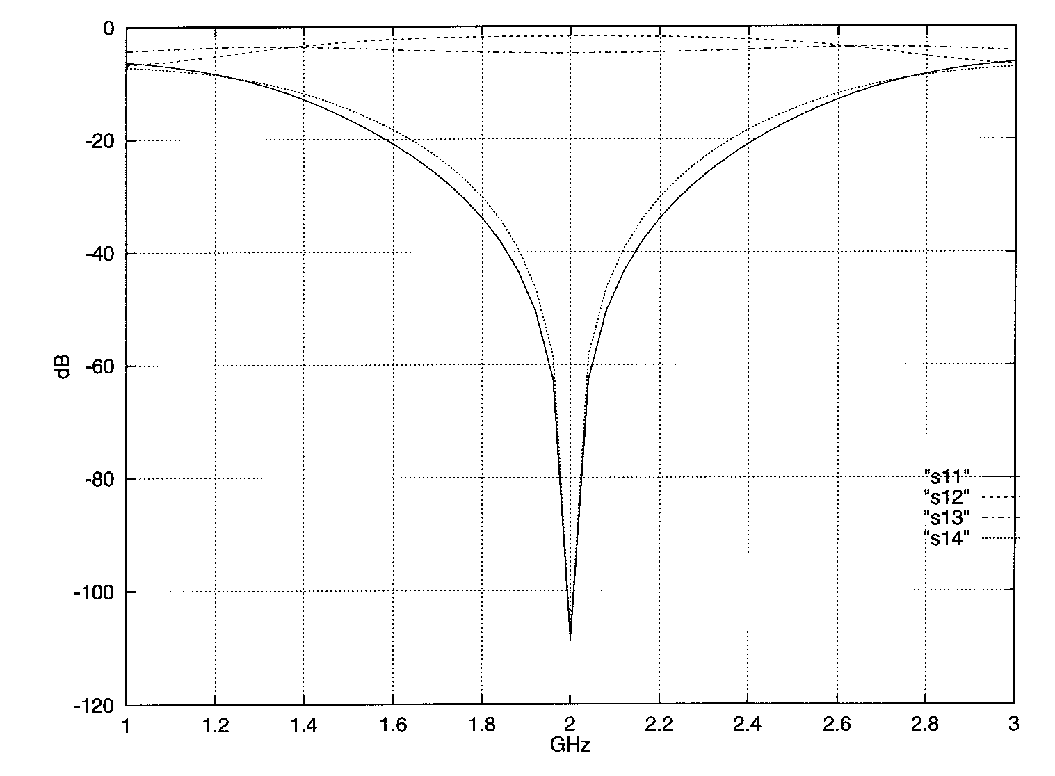
Figure 13: Computed response for the Butterworth synthesized 3 dB unequal power division 2 GHz hybrid ($r=1.2$) corresponding to Fig. 7. The impedance values are $a_{1}=152.44\Omega,a_{2}=66.05\Omega,a_{3}=195.31\Omega,b_{1}=43.55\Omega,b_{2}=48.03\Omega$.

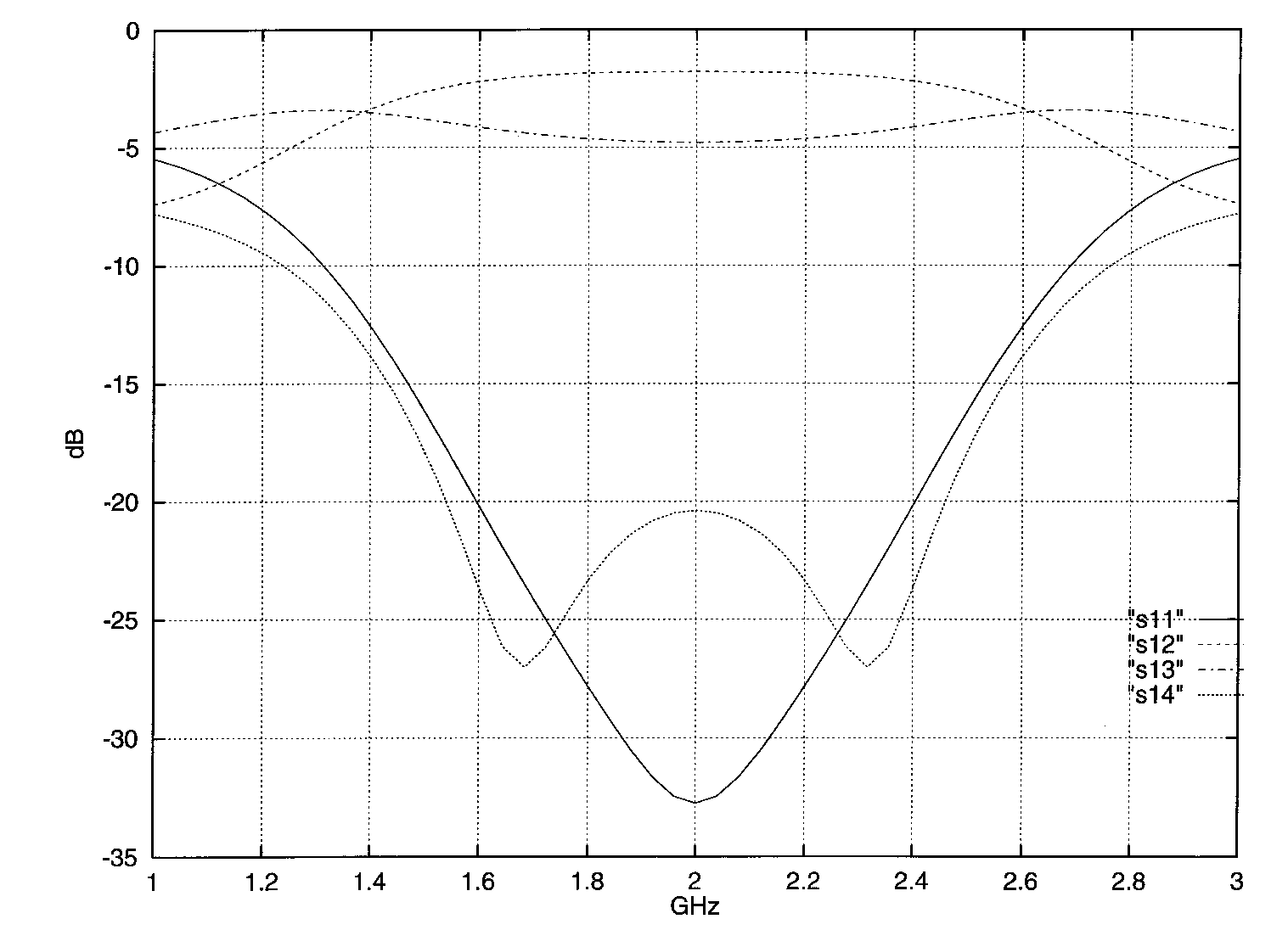
Figure 14: Computed response for the modified Chebyshev synthesized 3 dB unequal power division 2 GHz hybrid ($r=1.2$) corresponding to Fig. 7. The obtained isolation at midband is less than -20 dB. The impedance values are $a_{1}=153.89\Omega,a_{2}=61.30\Omega,a_{3}=153.89\Omega,b_{1}=b_{2}=41.63\Omega$.

The modified Chebyshev approach consists of calculating the parameters $K$ and $X_{c}$ by first assuming $r=1$. Once the $a_{i}$’s and $b_{i}$’s are obtained, the S parameters with the actual value of $r$ are calculated. The frequency response is displayed in Fig. 11. The required power division ratio (almost 0 dB) as well as good isolation (around -22.5 dB) were obtained. Experimental verification of the synthesized design was done by fabricating a microstrip hybrid on a 0.031 inch thick Duroid substrate. The measured responses displayed in Fig.11 indicate a very close agreement with the synthesis. The second example of Chebyshev type is the wide band two section impedance transformer ($50\Omega$ to 60 $\Omega$) with specified - 3dB power division at midband. This hybrid was optimized and the results were presented in Fig.7. In Fig. 12, all the S parameters for the Chebyshev synthesized hybrid are presented. In this case, the resulting impedance values are: $a_{1}=161.31\Omega,a_{2}=55.37\Omega,a_{3}=125.94\Omega,b_{1}=39.96\Omega,b_{2}=36.28\Omega$. The power division ratio was obtained from the synthesis as required (-3 dB) but a poor isolation (-15 dB) at midband was found. In contrast, the Butterworth synthesis is shown in Fig. 13. Synthesis was also done with the modified Chebyshev method mentioned above and the results are shown in Fig. 14. As may be seen, this modified method resulted in quite a reasonable response with an isolation better than 20dB.

IV CONCLUSIONS

Design equations for a two section impedance transforming quad hybrid were derived. Using these equations a two section branch line hybrid can be designed to achieve a percentage bandwidth of $30\%$ with impedance transformation by a factor of .7 to 1.3. Over this bandwidth the power balance between the output ports is measured better than 0.5 dB. A two section branch line hybrid with 3dB unequal power division also has a $30\%$ bandwidth but the impedance transformation ratio range drops to [0.833 - 1.2]. A slotline/lumped implementation of such a hybrid is attractive for MMIC circuits. In addition, a new general synthesis method for a multisection hybrid with Butterworth or Chebyshev response is described. Both symmetric (with equal input and output impedances) and non-symmetric (impedance transforming) designs were demonstrated. A close agreement between the synthesized, optimized and measured results were obtained.

Acknowledgement

The authors wish to thank G. Wells for assistance in fabrication and testing and P. Pramanick for many stimulating discussions. Financial support for this work was provided by the Natural Sciences and Engineering Research Council of Canada under a university industry chair program.

References

- (1) R. K. Gupta, S. E. Anderson and W. Getsinger: ”Impedance Transforming 3-dB 90 degrees Hybrid” IEEE MTT-35, 1303 (1987).
- (2) I. Telliez, A-M Couturier, C. Rumelhard, C. Versnaeyen, P. Champion, D. Fayol: ”A Compact Monolithic Microwave Demodulator-Modulator for 64 QAM Digital Radio Links” IEEE MTT-39, 1947 (1991).
- (3) W. A. Davis: ”Microwave Semiconductor Circuit Design” Van Nostrand Reinhold, New-York (1984).
- (4) L.F. Lind: ”Synthesis of Asymmetrical Branch Guide Directional Coupler Impedance Transformer”: IEEE MTT-17, 45 (1969).
- (5) H.J. Riblet: ”Comments on Synthesis of Symmetrical Branch Guide Coupler” IEEE MTT-18, 47 (1970).
- (6) R. Levy and L.F. Lind: ”Synthesis of Symmetrical Branch Guide Directional Couplers” IEEE MTT-16, 80 (1968).
- (7) G. C. Temes and J. W. Lapatra: ”Introduction to Circuit Synthesis and Design”, McGraw-Hill (New-York 1977).