How Many Genes Are Needed for a Discriminant
Microarray Data Analysis ?

Abstract

The analysis of the leukemia data from Whitehead/MIT group is a discriminant analysis (also called a supervised learning). Among thousands of genes whose expression levels are measured, not all are needed for discriminant analysis: a gene may either not contribute to the separation of two types of tissues/cancers, or it may be redundant because it is highly correlated with other genes. There are two theoretical frameworks in which variable selection (or gene selection in our case) can be addressed. The first is model selection, and the second is model averaging. We have carried out model selection using Akaike information criterion and Bayesian information criterion with logistic regression (discrimination, prediction, or classification) to determine the number of genes that provide the best model. These model selection criteria set upper limits of 22-25 and 12-13 genes for this data set with 38 samples, and the best model consists of only one (no.4847, zyxin) or two genes. We have also carried out model averaging over the best single-gene logistic predictors using three different weights: maximized likelihood, prediction rate on training set, and equal weight. We have observed that the performance of most of these weighted predictors on the testing set is gradually reduced as more genes are included, but a clear cutoff that separates good and bad prediction performance is not found.

Introduction

There are two types of microarray experiments. In the first type, samples are not labeled, but gene expression levels are followed with time. The goal is to find genes whose expression levels move together. In the second type, samples are labeled as either normal or diseased tissues. The goal is to find genes whose expression levels can distinguish different labels. Using terminology from machine learning, the data analysis of the first type of experiment is “unsupervised”, whereas that of the second type is “supervised” (see, e.g., [Haghighi, Banerjee, Li, 1999]). The prototype of the first type of analysis is cluster analysis, whereas that of the second type is discriminant analysis.

We focus on the data analysis of the second type, using the leukemia data from Whitehead/MIT’s group [Golub et al, 1999]. The question we are addressing is how many gene expressions are needed for a discriminant analysis. In this data set, 7129 gene expressions are measured on 38 sample points. In the original analysis [Golub et al, 1999], 50 out of more than 7000 gene expressions are used for discriminant analysis. We ask whether 50 genes are still too large a number, considering that the sample size is only 38. This seemingly simple question may receive two answers from two different perspectives: model selection (see, e.g., [Burnham, Anderson, 1998]) and model averaging (see, e.g., [Geisser, 1974]). We will address the two separately below.

Model Selection

The goal of model selection is to pick the model among many possible models that achieves the best balance between data-fitting and model complexity. A perfect data-fitting performance by a complicated model with many parameters can well be an example of overfitting. On the other hand, a simplistic model with few parameters that fits the data poorly is an example of underfitting. There are two proposals for achieving the balance between data-fitting and model complexity: Akaike information criterion (AIC) [Akaike, 1974; Parzen, Tanabe, Kitagawa, 1998; Burnham, Anderson, 1998] and Bayesian information criterion (BIC) [Schwarz, 1976; Raftery, 1995]. These two quantities are defined as:

$$\mbox{AIC}=-2\log(\hat{L})+2K,\hskip 14.45377pt\mbox{ and}\hskip 14.45377pt\mbox{BIC}=-2\log(\hat{L})+\log(N)K,$$ (1)

where $\hat{L}$ is the maximized likelihood, $K$ the number of free parameters in the model, and $N$ the sample size. High-order terms of $O(1/N)$ (for AIC) and $O(1)+O(1/\sqrt{N})+O(1/N)$ (for BIC) are ignored here for simplicity. The model with the lowest AIC or BIC is considered to be the preferred model.

Selecting genes relevant to a discriminant microarray data analysis may become an issue of model selection. But we have to be clear in what context this is the case. Model selection adjusts the number of parameters in the model, not the number of variables. Nevertheless, if we plan to combine variables (additively or any other functional form), each variable has one or perhaps more coefficient. Removing a variable removes the corresponding coefficient. In this context, variable selection is a special case of model selection. We illustrate this by the logistic regression/discrimination for our data set:

$$\mbox{Prob(AML)}=\frac{1}{1+e^{-a_{0}-\sum_{j\in top\hskip 3.61371ptgenes}a_{j}x_{j}}}$$ (2)

where $x_{j}$ is the (log, normalized) gene expression level of gene $j$ among the top performing genes, and AML (acute myeloid leukemia) is one type of leukemia (ALL, the acute lymphoblastic leukemia, is another type). Using a linear combination of all 7129 genes in logistic discrimination requires 7130 parameters, whereas using one gene requires only 2 parameters. AIC/BIC defined in Eq.(1) will then compare multiple-gene models with single-gene models, and determine which scenario is better.

Our results are summarized in Table 1, where we list the type of model (which variables are additively combined in the logistic regression), number of parameters in the model, -2log of the maximum likelihood, AIC/BIC (absolute and relative), prediction rate in training set, and that in the testing set. The most striking result from this data set is that many genes are strong predictors for the leukemia class, consistent with the observation in [Golub et al, 1999]. This observation is confirmed by the following facts in Table 1: logistic regressions using the top 2, 5, 10, 22,and 37 genes all fit the data almost perfectly (as measured by the $-2\log(\hat{L})$ value) (note that the model is saturated when the number of variables used in the logistic regression is 37, since the number of parameters is then equal to the number of sample points); stepwise variable selection leads to only two genes (note that stepwise variable selection fails to find the best model, a single-gene model, because it is a local minimization/maximization procedure); the No.10 best-performing gene is only slightly worse than the No.1 performing gene: 35 vs. 36 correct predictions on the training set (though the No.100 and No.200 best-performing genes predict only 30 and 29 correctly on the training set); etc. This situation of strong prediction or easy classification is in contrast with the epidemiology and pedigree data used in human complex diseases, where strong predictors are rather rare [Li, Sherriff, Liu, 2000; Li, Nyholt, 2001].

Thest two rows in Table 1 are predictors/classifiers that do not use any gene expression levels. These are random guesses or null models. The first null model (#1) uses the proportion of AML in all samples as Prob(AML) (11/38 in our training set) as the guessing probability for AML. The second null model (#0) uses half-half probabilities. It is interesting to note that to beat both null, the number of genes in logistic regression can not exceed some upper limits: for null model 1, since we require AIC/BIC to be smaller (where $p$ is the number of genes used in logistic regression, and $-2\log(\hat{L})$ is assumed to be zero for the best-case scenario):

$$0+2(p+1)\approx\mbox{AIC} < \mbox{AIC (fixed)}=47.728$$

$$0+3.637568(p+1)\approx\mbox{BIC} < \mbox{BIC (fixed)}=49.365,$$ (3)

it sets $p<22.86\approx 22$, and $p<12.57\approx 12$, respectively. Similarly, to beat the random-guess model, we require:

$$0+2(p+1)\approx\mbox{AIC} < \mbox{AIC (random)}=52.679$$

$$0+3.637568(p+1)\approx\mbox{BIC} < \mbox{BIC (random)}=52.679$$ (4)

which are $p<25.34\approx 25$, and $p<13.48\approx 13$, respectively. These specific upper limits are directly related to the fact that the sample size is 38. They will move up and down with the sample size.

type	K	-2log($\hat{L}$)	AIC	$\Delta$AIC	BIC	$\Delta$BIC	$p_{train}$	$p_{test}$
#1 g4847 (zyxin)	2	5$\times$10-9(a)	4.000	0	7.275	0	38/38	31/34
#2 g1882 (CST3 cystatin C)	2	6.973	10.973	6.973	14.248	6.973	36/38	32/34
#3 g3320 (leukotriene c4 synthase)	2	10.914	14.914	10.914	18.190	10.915	35/38	27/34
#4 g5039 (LEPR leptin receptor)	2	11.355	15.355	11.355	18.630	11.355	36/38	22/34
#5 g6218 (ELA2 elastatse 2)	2	11.459	15.459	11.459	18.734	11.459	34/38	22/34
#6 g2020 (FAH ..)	2	12.103	16.103	12.103	19.378	12.103	36/38	25/34
#7 g1834 (CD33 antigen)	2	12.226	16.226	12.226	19.501	12.226	35/38	31/34
#8 g760 (cystatin A)	2	13.104	17.104	13.104	20.379	13.104	35/38	32/34
#9 g1745 (LYN v-yes-1..)	2	13.151	17.151	13.151	20.426	13.151	33/38	28/34
#10 g5772 (c-myb)	2	14.723	18.723	14.723	21.998	14.723	35/38	27/34
#100 g2833(AF1q)	2	27.215	31.215	27.215	34.490	27.215	30/38	28/34
#200 g3312(protein kinase ATR)	2	30.841	34.841	30.841	38.117	30.842	29/38	21/34
g1834+g2267(b)	3	0.004	6.004	2.004	10.917	3.642	38/38	22/34
g5039+g5772(c)	3	0.008	6.008	2.008	10.921	3.646	38/38	26/34
top 2 (g4847+g1882)	3	0.029	6.029	2.029	10.942	3.667	38/38	32/34
top 5	6	0.011	12.011	8.011	21.837	14.562	38/38	24/34
top 10	11	0.002	22.002	18.002	40.016	32.741	38/38	31/34
top 22	23	0.001	46.001	42.001	83.666	76.391	38/38	27/34
top 37	38	0.001	76.001	72.001	138.229	130.954	38/38	21/34
null 1 (proportion estimation)	1	45.728(d)	47.728	43.728	49.365	42.090	27/38(d)	20/34(d)
null 0 (random guess)	0	52.679(e)	52.679	48.679	52.679	45.404	19/38(e)	17/34(e)

Table 1: Logistic regression results (sample size N=38, log(N)=3.637568). $K$: number of free parameters in the logistic regression (LR) (number of genes included plus 1); $\Delta$AIC ($\Delta$BIC) is the AIC (BIC) value relative to that of the best model (single-gene LR using g4847, zyxin); $p_{train}$ ($p_{test}$) is the prediction rate on the training (testing) set; “top 37” is the LR using 37 best genes by their single-variable LR performance. Notes (a) Since this model/predictor fits the data perfectly, $\hat{L}$ should be 1, and $-2\log(\hat{L})$ should be 0. In a real optimization procedure, the actual value may depend on the number of iterative steps. (b) This LR is selected by a stepwise variable selection (by either AIC or BIC) from the starting group of top 22 genes (top 22 $\rightarrow$ A/BIC $\rightarrow$ 2); (c) Similar to (b), but the starting group of genes in the LR containing the top 10 genes (top 10 $\rightarrow$ A/BIC $\rightarrow$ 2); (d) This null model uses 11/38 $\approx$ 0.29 as the probability for AML for any sample data. Since 0.29 $<$ 0.5, any sample will be predicted as ALL type, which is correct 27 times in the training set, and 20 times in the testing set. The $-2\log(\hat{L})$ is equal to $-2\log[(27/38)^{27}(11/38)^{11}]$; (e) The $-2\log(\hat{L})$, $p_{train}$, and $p_{test}$ for the random guess model is expected to be: $-2\log(0.5^{N})=2N\log(2)$, 0.5, and 0.5.

Model Averaging

In the model selection framework, we can not use a logistic regression with too many genes because it may not improve the data-fitting performance enough to compensate for the increase of model complexity. This conclusion is correct when one model (e.g. a logistic regression that uses one gene) is compared to other alternative models (e.g. a logistic regression that uses, say, 10 genes). Nevertheless, it is possible to average/combine many different models each involving one gene. The restriction on model complexity during the model selection process does not apply to model averaging. Model averaging has also been discussed under names such as “committee machines”, “boosting weak predictors”, “mixture of experts”, “stacked generalization” (see, e.g., [Ripley, 1996]).

Without guidance from the model selection framework on the number of models (number of genes) to be included, we have tried several empirical approaches. We first examine whether there is a gap in data-fitting performance among top genes. Genes that do not fit the data should not be considered in model averaging. For this purpose, Fig.1 shows the $-2\log(\hat{L})$ for the top 1000 genes on the training set, as a function of the (log) rank. A linear fitting of $-2\log(\hat{L})$ on $\log$(rank) seems to fit the points well, and it is hard to see “better-than-average” genes except the first gene. This is not surprising since g4847 discriminates the 38 training sample points perfectly. Note that the linear trend in Fig.1 is equivalent to a power-law function in likelihood vs. rank plot ( $\hat{L}\sim 1/r^{2.56}$). Such power-law is similar to the power-law rank-frequency plots observed in many social and natural data, also known as Zipf’s law [Zipf, 1949; Li, 1997-2001]. In any case, there is no discernible gap in Fig.1 that separates relevant and irrelevant genes.

We then check how the prediction rate on the training set correlates with that on the testing set. Fig.2 shows the error rates on both training (x-axis) and testing sets (y-axis) for the top 500 performing genes. The left plot in Fig.2 shows the mean square error, and the right plot shows the prediction errors. The left plot contains both information on the success rate of prediction and that of confidence of prediction, whereas the right plot contains only information on the success rate of prediction. Points along the diagonal line in Fig.2 exhibit similar error rates in the training and testing set, and thus are reasonable predictors. On the other hand, points well above the diagonal line indicate overtraining. The most reasonable predictor based on both the training and testing set is g1882 (on the other hand, the best predictor based on training set is g4847).

Finally we examine the model averaging performance with various numbers of models included, each being a single-gene logistic regression:

$$\mbox{Prob(AML)}=\sum_{j\in\mbox{top genes}}w_{j}\left(\frac{1}{1+e^{-a_{j}-b_{j}x_{j}}}\right).$$ (5)

We have chosen three weighting schemes: the first is proportional to the prediction rate on the training set ($w_{j}\propto p_{j,train}$), the second is the equal weight ($w_{j}\propto 1$), and the last one is proportional to the maximum likelihood as obtained from the training set ($w_{j}\propto\hat{L}_{j}$). Fig.3-4 shows the behavior of all three weighting schemes on both the training and the testing sets, using either the mean square error or the prediction error, up to 200 genes.

The maximum likelihood weight is equivalent to the Akaike weight ($w_{j}\propto exp(-\mbox{AIC}_{j}/2)$) [Parzen, Tanabe, Kitagawa, 1998] and Bayesian weight ($w_{j}\propto exp(-\mbox{BIC}_{j}/2)$) [Raftery, 1995], since all models being averaged in Eq.(5) have the same number of parameters and same sample size (assuming high-order terms are ignored). Using Bayesian weight in model averaging is essentially a derivation of the posterior predictive distribution [Gelman, et al, 1995]: “posterior” because data in a training set is used, and “predictive” because unknown new data in the testing set is to be predicted.

For our data set, this weighting scheme is nevertheless uninteresting: the mean square error only decreases slightly with the number of models used, while the error in prediction rate is unchanged. The reason for this is very simple: the best model (the single-gene logistic regression using the g4847) discriminates the training set perfectly. Its likelihood is much higher than any other models. As a result, the weight of other models is negligible, and the model averaging essentially remains as one model. The equal weight can be potentially incorrect since models that do not fit the data should not contribute as equally as models that fit the data better. In our data set, however, the equal weight scheme is actually similar to the weighting scheme that uses the prediction rate, because many genes (up to 200) exhibit similar prediction rates on the training set.

It is difficult from Fig.3-4 to determine a cutoff on the number of models (number of genes) to be included. Fig.3-4, however, clearly shows that a lower number of models (genes) is typically better (except the maximum likelihood weight, which is insensitive to the number of genes included). Fig.3, in particular, indicates that it is possible to perform better (in term of mean square error) on the testing set than using just one model if the number of models is less than around 25. Of course, this result is obtained from the specific testing set we have at hand. A more conclusive result may require a combining of the training and testing set, or requires more sample points than are currently available.

Due to the weight in a model averaging, the apparent number of terms (models, genes) included does not reflect on the true number of genes involved. For this reason, we may introduce a quantity called “effective number of genes (terms, models)”. The leading term in a model averaging contributes a number of 1 to this quantity, but the contribution from the term j is equal to $w_{j}/w_{1}$. For example, with the maximum likelihood weight, the relative weights of the first ten terms are 1, 0.031, 0.0043, 0.0034, 0.0032, 0.0024, 0.0022, 0.0014, 0.0014, and 0.0006. The effective number of terms when the top ten genes are included is 1.05, a far less number than 10.

The discrimination used in [Golub et al, 1999] is a model averaging instead of a model selection. The number of genes used is 50. To quote from [Golub, et al, 1999], “the number was well within the total number of genes strongly correlated with the class distinction, seemed likely to be large enough to be robust against noise, and was small enough to be readily applied in a clinical setting.” Our Fig.3-4 shows that although the prediction rate on the training set stays close to 100% even as the number of models (genes) is increased, the prediction rate on the testing set decreases with more genes. The only exception is the maximum likelihood weight, where the prediction rate is almost unchanged due to the dominance of the best gene. It seems that we should not increase the number of models (genes) in model averaging arbitrarily.

In conclusion, due to the small sample size and the presence of strong predictors, we believe the number of genes used in a discriminant analysis in this data set can be much smaller than 50. Although we can not give a definite answer as to the exact number of genes to be used, one proposal is to use only one or two genes, and other exploratory data analyses indicate an upper limit of 10-20 genes. Similar analysis of other data sets for cancer classifications using microarray will be discussed in [Li, et al. 2001] and Zipf’s law in these data sets will be discussed in [Li, 2001].

References

H Akaike (1974), “A new look at the statistical model identification”, IEEE Transactions on Automatic Control, 19:716-723.

KP Burnham, DR Anderson (1998), Model Selection and Inference (Springer).

A Gelman, JB Carlin, HS Stern, DB Rubin (1995), Bayesian Data Analysis (Chapman & Hall).

S Geisser (1993), Predictive Inference: An Introduction (Chapman & Hall).

TR Golub, DK Slonim, P Tamayo, C Huard, M Gaasenbeek, JP Mesirov, H Coller, ML Loh, JR Downing, MA Caligiuri, CD Bloomfield, ES Lander (1999), “Molecular classification of cancer: class discovery and class prediction by gene expression monitoring”, Science, 286:531-537.

F Haghighi, P Banerjee, W Li (1999), “Application of artificial neural networks in whole-genome analysis of complex diseases” (meeting abstract), Cold Spring Harbor Meeting on Genome Sequencing & Biology, page 75.

W Li (1997-2001), An online resource on Zipf’s law (URL: http://linkage.rockefeller.edu/wli/zipf/).

W Li (2001), “Zipf’s law in importance of genes for cancer classification using microarray data”, submitted.

W Li, A Sherriff, X Liu (2000), “Assessing risk factors of complex diseases by Akaike information criterion and Bayesian information criterion” (meeting abstract), American Journal of Human Genetics, 67 (supp 2), page 222.

W Li, D Nyholt (2001), “Marker selection by AIC/BIC”, Genetic Epidemiology, in press.

E Parzen, K Tanabe, G Kitagawa (1998), Selected Papers of Hirotugu Akaike (Springer).

AE Raftery (1995), “Bayesian model selection in social research”, in Sociological Methodology, ed. PV Marsden (Blackwells), pages 185-195.

BD Ripley (1996), Pattern Recognition and Neural Networks (Cambridge University Press).

G Schwarz (1976), “Estimating the dimension of a model”, Annals of Statistics, 6:461-464.

GF Zipf (1949), Human Behavior and the Principle of Least Effect (Addison-Wesley).

Figure 1: Data-fitting performance as measured by $-2\log(\hat{L})$ (the smaller, the better fit) for the top 1000 genes. The x-axis is the rank of the gene by the likelihood of its single-gene logistic regression. A linear regression line of $-2\log(\hat{L})$ vs. $\log$(rank) is also shown, with the slope equal to 5.12.

Figure 2: Error rates on the testing set (y-axis) are compared with those on the training set (x-axis) for the top 500 genes (based on the performance on the training set). Each point represents one single-gene logistic regression predictor. The left plot uses the mean squared error (“+” for the first 50 top genes, “-” for the top 51-100 genes, “*” for the top 101-200 genes, and “.” for the top 201-500 genes), and the right plot uses the prediction error.

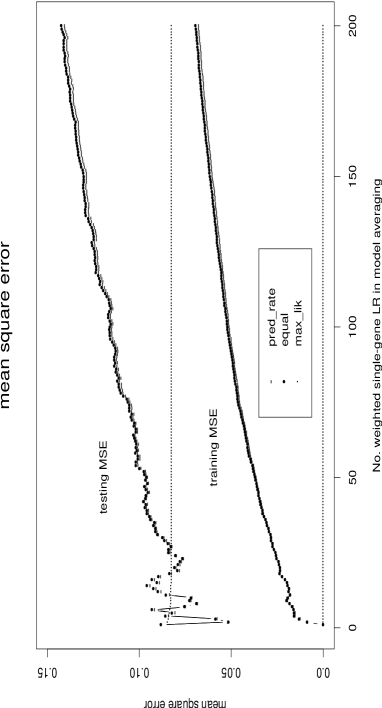
Figure 3: Model averaging performance with three different weighting schemes: (1) weight being proportional to the prediction rate on the training set; (2) equal weight; and (3) weight being proportional to the maximum likelihood obtained on the training set. The mean square error is plotted against the number of models being averaged. Each model is a single-gene logistic regression. The mean square error on both the training set (bottom) and the testing set (top) are shown.

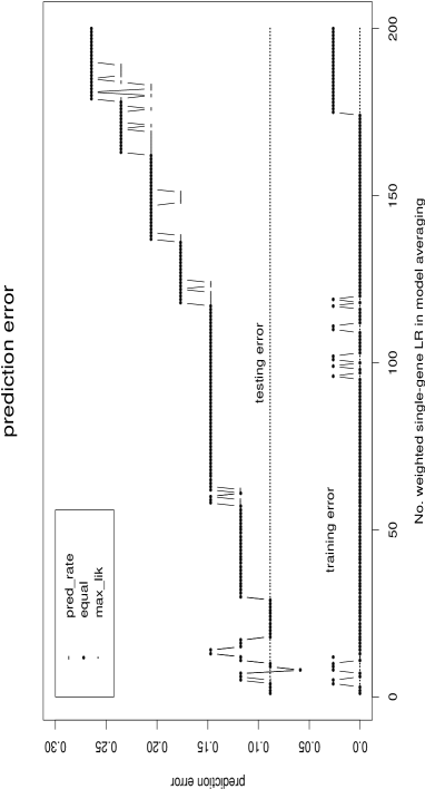
Figure 4: Similar to Fig.3, but the prediction error rate is plotted against the number of models being averaged (each model is a single-gene logistic regression).