Zipf’s Law in Importance of Genes for Cancer Classification
Using Microarray Data

Abstract

Microarray data consists of mRNA expression levels of thousands of genes under certain conditions. A difference in the expression level of a gene at two different conditions/phenotypes, such as cancerous versus non-cancerous, one subtype of cancer versus another, before versus after a drug treatment, is indicative of the relevance of that gene to the difference of the high-level phenotype. Each gene can be ranked by its ability to distinguish the two conditions. We study how the single-gene classification ability decreases with its rank (a Zipf’s plot). Power-law function in the Zipf’s plot is observed for the four microarray datasets obtained from various cancer studies. This power-law behavior in the Zipf’s plot is reminiscent of similar power-law curves in other natural and social phenomena (Zipf’s law). However, due to our choice of the measure of importance in classification ability, i.e., the maximized likelihood in a logistic regression, the exponent of the power-law function is a function of the sample size, instead of a fixed value close to 1 for a typical example of Zipf’s law. The presence of this power-law behavior is important for deciding the number of genes to be used for a discriminant microarray data analysis.

1 Introduction

Not all of the more than 30,000 human genes and perhaps a multiple of that number of proteins [Venter, et al., 2001; IHGSC, 2001] are expected to be useful for all situations. For a specialized phenotype, a particular genetic disease, or a biological process of interest, only a portion of the genes are involved. Even for the involved genes, their contribution to that phenotype (or disease, or process) varies: some genes can be more important than others. The number of genes involved in a phenotype/disease/process also differs from one case to another: some phenotypes require a large number of genes to contribute (polygenic), others may only need a few (oligogenic). This theme has been discussed in the study of human genetic diseases: those caused by mutation in one gene are called Mendalian or simple diseases, whereas those caused by multiple mutations in many genes, or due to an interplay between genetic susceptibility and environmental factors, are called complex genetic diseases (see, e.g., [Haines, et al., 1998]).

Once a phenotype, a disease, or a biological process has been chosen, we may examine each gene’s contribution to the phenotype/disease/process under study, and its “importance” can be ranked. This ranking is a very common practice in quantitative analyses of natural and social phenomena. For example, cities can be ranked by their population, companies can be ranked by revenue or profit, ecological disasters can be ranked by the population of species being destroyed, etc. Plotting the measurement by which the ranking is determined, versus the ranking number (1 for the best or the largest, etc., 2 for the second-best, $\cdots$) is called a Zipf’s plot, originated from the work of George Zipf [Zipf, 1935, 1949].

Among the large number of Zipf’s plots drawn by Zipf, especially that of the frequency of word occurrence in human language, it was observed that they tend to follow a power-law (algebraic) function: $y\sim 1/r^{\alpha}$, where $r$ is the rank, $y$ is the measurement that determines the rank, and $\alpha\approx 1$ the scaling exponent. This power-law behavior is called Zipf’s law. Power-law Zipf’s plot where the value of $\alpha$ is not close to 1 may be called a generalized form of Zipf’s law. Examples of Zipf’s law, besides those mentioned above, include magnitude of earthquakes [Sornett, et al., 1996], popularity of webpage visits [Crovella & Bestavros, 1997], usage of library books, frequency of key word search [Chen & Leimkuhler, 1986], etc. More references on Zipf’s law can be found at an online resource at http://linkage.rockefeller.edu/wli/zipf.

This paper addresses the question of whether human genes can be ranked by their “importance” in their contribution to a particular phenotype such as cancer. Once a measurement of the importance of a gene is defined, we ask whether this measure of importance as a function of the rank follows an inverse power-law function, i.e. Zipf’s law. There are two aspects of this study. Qualitatively, Zipf’s plot will show whether or not the importance of genes, at least for a particular phenotype classification task, follows a continuous spectrum. A discontinuous gap would separate “important” genes from “unimportant” ones. Quantitatively, how fast the importance of genes falls off as a function of the rank provides information on how many genes should be kept for this phenotypic classification.

The invention of the microarray (DNA chip) was a breakthrough in biotechnology (see, e.g., [Southern, 1996; Ekins & Chu, 1999]), which makes it possible to monitor the expression level of thousands of gene products such as mRNA simultaneously. A comparison of these gene expression levels in cancerous as well as normal tissues will point to genes relevant to oncogenesis. When each gene is examined individually, the more its expression is different in cancerous tissues from that in normal tissues, the more relevant this gene is to cancer development, and the more important it is for cancer classification. In this paper, we use microarray data to rank the importance of genes, and Zipf’s plot of this measure of importance is studied. Section 2 introduces the mathematical formula and quantities used in this paper; section 3 illustrates the likelihood-rank plots (Zipf’s plot) for the simplest cancer classifications (two-type); section 4 shows the Zipf’s plot for multiple-type classifications; section 5 shows the Zipf’s plot for paired samples classification; section 6 discusses the issue concerning the exponent in the power-law plot; and section 7 contains other discussions.

2 Measure of importance of genes in cancer classification: likelihood

The measurement we use for the importance of genes in cancer classification is the maximized likelihood, which is proportional to the probability of observing the data when a model is given, and when the parameters in the model are adjusted to give the maximum value. Mathematically, likelihood $L$ is [Edwards, 1972]:

$$L=cP(D|M,\theta),$$ (1)

where $D$ is all data points in a data set, $M$ is a model, $\theta$ represents all parameters in the model, and $c$ is a proportional constant (often set to be 1). The maximized likelihood is

$$\hat{L}=\max_{\theta}L=cP(D|M,\hat{\theta}),$$ (2)

where the $\hat{}$ represents a maximization/estimation procedure. The microarray data sets have the form of $\{x_{1i},x_{2i},\cdots,x_{pi},y_{i}\}$ ($i=1,2,\cdots N$). Each sample point $i$ (one microarray experiment, one tissue sample) contains measurements of (logarithm of ) mRNA expression level of $p$ genes ($p$ is typical of the order of thousands), and $y$ is a categorical label indicating a condition (e.g. cancerous or normal). The raw data in a microarray experiment could be more complicated: one has to consider background noise, normalization, and controls. These considerations depend on the type of chips: Stanford/cDNA array with two fluorescence dyes [Schena, et al., 1995; Shalon et al., 1996] or Affymetrix/oligonucleotide arrays with only one image intensity to measure but multiple oligonucleotide probes [Fodor, et al., 1991]. In this paper, only the filtered/processed data are used and the subtle issue of scaling/normalization of the raw data is not discussed.

The model $M$ is a classification model (classifier, predictor, discriminator, supervised learning machine), that classifies the label $y$ by the gene expression level $\{x_{j}\}$ (logarithm of an image intensity from the DNA chip). We use a particularly simple classifier, the single-gene logistic regression:

$$P(y_{i}=1|x_{ji})=\frac{1}{1+e^{-a_{j}-b_{j}x_{ji}}}.\hskip 7.22743pt\mbox{$j=1,2,\cdots p$, and }\hskip 7.22743pt\mbox{$i=1,2,\cdots N.$ }$$ (3)

In other words, the probability of a sample being in one class is a “sigmoid” or “logistic” function of the (log) expression level. If the coefficient $b$ is positive, larger expression levels lead to higher probabilities of being the $y=1$ label; if $b<0$, larger expression level corresponds to the $y=0$ label.

The likelihood of the whole data set is the product of these model-based probabilities (for a given gene):

$$L_{j}=\prod_{i=1}^{N}\left[P(y=1|x_{ji}){\bf I}_{y_{i}=1}+(1-P(y=1|x_{ji})){\bf I}_{y_{i}=0}\right],\hskip 7.22743pt\mbox{$j=1,2,\cdots p$ }$$ (4)

where ${\bf I}$ is the indicator function (1 or 0 depending on whether the condition is true or not). Eq.(4) is maximized by adjusting the parameters in the model. The maximized likelihood $\hat{L}$ can then be used to rank all genes: the larger the $\hat{L}$, the higher the ranking.

3 Zipf’s plot of classification likelihood

The binomial (two-class) logistic regression Eq.(3) has been applied to two microarray data sets. The first is colon cancer data from Princeton University [Alon, et al., 1999]. The expression levels of 2000 genes were available for 62 tissue samples: 40 cancerous and 22 normal. The second data set is leukemia data from Whitehead Institute/MIT [Golub, et al., 1999]. Expression levels of 7129 genes were measured on 72 leukemia samples: 47 obtained from tissues of one subtype of leukemia, acute lymphoblastic leukemia (ALL), and 25 from tissues of another subtype of leukemia, acute myeloid leukemia (AML). Although the number of labels is 2 for both datasets, we distinguish cancerous from normal tissues in the first data set, whereas distinguish one cancer subtype from another in the second data set.

For the colon cancer data, the single-gene maximized likelihood Eq.(4) for each gene was calculated and ranked. The likelihood-rank plot (Zipf’s plot) is shown in Fig.1 in log-log scale. The power-law behavior of the curve is clearly visible. Fitting the first 600 genes using a generalized form of Zipf’s law:

$$\hat{L}_{r}\sim 1/r^{\alpha},$$ (5)

leads to exponent $\alpha\approx 2.18$, whereas the fitting of the top 1000 genes leads to $\alpha\approx 2.10$. The genes from roughly rank 1000 to 2000 do not seem to follow the same power-law decay of the likelihood. As will be discussed more later in this paper, the exponent $\alpha$ is not an intrinsic quantity for our likelihood-rank plots. The reason is that the likelihood is a product of probabilities of $N$ sample points $L_{r}\propto(p_{1}p_{2}\cdots p_{N})_{r}\sim\bar{p}_{r}^{N}$; if the per-sample averaged likelihood $\bar{p}_{r}$ of rank-r gene does not change with the sample size $N$, the exponent $\alpha$ is then a function of $N$: $\alpha\sim-N\log(\bar{p}_{r})/log(r)$.

Fig.2 shows the Zipf’s plot of the second data set. Among the 72 samples, 38 are from bone marrow tissues, and were separated as a training set in [Golub, et al., 1999]. These 38 samples were considered to be more homogeneous, while the rest of the samples were from various sources or other tissue types such as peripheral blood [Golub, et al., 1999], and may not be homogeneous. From Fig.2, the Zipf’s plot obtained from the training set seems to follow a generalized form of Zipf’s law with a fitting exponent of $\alpha\approx 2.56$ from the top 900 genes. The Zipf’s plot of all sample points seems to deviate from a power-law trend around rank 100-200. As mentioned earlier, the exponent $\alpha$ from a bigger data set is indeed larger than the exponent from a small data set.

When the top genes are examined, it was found that the top-ranking genes for the training set [Li & Yang, 2001] and those for the overall set [Li, et al., 2001] may not be identical. For example, the top performing gene for the 38-sample training set is No.4847, zyxin, a gene encoding the LIM domain protein used in cell adhesion in fibroblasts [Golub, et al., 1999]. On the other hand, the best performing gene for the 72-sample combined set is No. 1834, CD33 antigene which encodes cell surface proteins commonly found in AML leukemia cells (see, e.g., [Lauria, et al., 1994]). The zyxin becomes the rank-4 gene for the combined dataset. This difference reflects a certain degree of inhomogeneity between samples in the training set and those in the remaining set (testing or validation set). Note from Fig.1 that for the training set, genes from rank 3 to 9 exhibits similar likelihood, and form a flat step on the Zipf’s plot. Such steps are a dominant feature in the Zipf’s plot of the frequency of word occurrence in randomly generated texts [Li, 1992].

4 Classification of multiple cancer classes

The logistic regression Eq.(3) for a two-class data set can be generalized to multiple classes: multinomial logistic regression [Agresti, 1996]:

$$P(y_{i}=I|x_{ji})=\frac{e^{-a_{I}-b_{I}x_{ji}}}{\sum_{K=1}^{C}e^{-a_{K}-b_{K}x_{ji}}}\hskip 14.45377pt\mbox{$j=1,2,\cdots p$, $I=1,2,\cdots C$, $i=1,2,\cdots N$,}$$ (6)

where the label $y$ can be in one of the $C$ classes, and there are two parameters for each class (though only $C-1$ class probabilities are independent). A gene is important (higher maximized likelihood) if it is more able to distinguish all $C$ classes simultaneously.

For this multiple-class analysis, we use the microarray data for lymphoma (Stanford University and National Cancer Institute [Alizadeh, et al., 2000]). There are a total 96 tissue samples, with 66 cancerous and 30 normal. Within the cancer samples, there are 46 diffuse large B-cell lymphoma (DLBCL), 9 follicular lymphoma (FL), 11 chronic lymphocyte leukemia (CLL). These 3 cancer subtypes plus the normal are the 4 classes to be distinguished. In [Alizadeh, et al., 2000], it is also recommended that two new subclasses of DLBCL can be defined based on the microarray data. These are the germinal centre B-like DLBCL (GC-DLBCL) and the activated B-like DLBCL (A-DLBCL). The GC-DLBCL, A-DLBCL subclasses plus the normal can be the 3 classes to be distinguished.

Fig.3 shows the Zipf’s plot of multinomial logistic regression likelihood for both the 4-class and the 3-class classification. The Zipf’s plot for the 3-class multinomial logistic regression follows a perfect power-law function for all genes. No deviation from power-law behavior was observed even for the low-ranking genes. The Zipf’s plot for the 4-class multinomial logistic regression, on the other hand, does not seem to follow a power-law function. The fall off near the rank-200 gene is perhaps due to the computer roundoff error since the value of likelihood at rank-200 is already as low as $10^{-39}$ (the likelihood is multipled by $10^{10}$ in Fig.3). The fitting of the top 200 genes by a power-law function is, however, very good.

5 Cancer treatment effect

Another interesting situation is provided by the data set from Stanford University and the Norwegian Radium Hospital [Perou, et al., 2000]. Part of the data is the expression level of 8102 genes measured before and after a 16-week course of doxorubicin chemotherapy [Perou, et al., 2000] on 20 patients. Naively, one may consider these 40 microarray experiments as an example of binary logistic regression. However, logistic regression in Eq.(3) does not apply because it requires samples to be independent of each other, whereas microarray experiments done on the same patient are clearly not independent. This situation can be handled by the logistic regression of paired case-controls (case is a sample with label 1, and control is a sample with label 0) [Breslow & Day, 1980]:

$$P(x(case)_{ji}-x(control)_{ji})=\frac{1}{1+e^{b_{j}(x(case)_{ji}-x(control)_{ji})}},\hskip 7.22743pt\mbox{$j=1,2,\cdots p$, $i=1,2,\cdots N$. }$$ (7)

Note that the probability is no longer that for observing $y$ – when a case sample and a control sample are paired, their $y$ value is fixed at 1 and 0 – but that of observing the difference of $x$’s. Also note that the first parameter $a$ is now zero.

Fig.4 shows the Zipf’s plot for genes in the breast cancer microarray data. The top three genes were able to perfectly identify the chemotherapy effect – the expression level is always higher (or lower) before the treatment than after in all 20 samples. The likelihood of a perfect fit is equal to 1. Unlike the previous three plots, the likelihood of genes in Fig.4 does not follow a power-law function, or even a smooth function. There seems to be a gap from the ranking of 19 to the ranking of 20-25. Fitting the two segments (from 4 to 19, and from 25 to 500) by power-law functions leads to different exponents (2.51 versus 1.77).

Plots like Fig.4 can be good news for a microarray data analysis, because there seems to be a separation between “relevant” and “irrelevant” genes. Irrelevant genes are not important for distinguishing samples before and after chemotherapy, and may be discarded for further analysis. Of course, this is only a rough description of the gene set. A more systematic approach can be based on the framework of model selection (see, e.g., [Burnham & Anderson, 1998]) or model averaging (see, e.g., [Geisser, 1993]). With model selection, the expression level of different genes can be combined, and adding one gene increases the number of parameters in the model by 1. The appropriate number of genes to be included in a classification is the model with the best “model selection criterion” such as Akaike information criterion [Burnham & Anderson, 1998] or Bayesian information criterion [Raftery, 1995], with a best balance between a larger likelihood value and fewer numbers of parameters [Li & Yang, 2001, Li, et al., 2001]. With model averaging, there is in principle no limitation on the number of genes to be included, but irrelevant genes have smaller weights in an averaged classifier [Golub, et al., 1999, Li & Yang, 2001]. This makes the effective number of genes used much smaller than the apparent number.

6 Scaling exponent

As mentioned earlier, the exponent of the inverse power-law fitting function for Zipf’s plot (Figs. 1-4) depends on the sample size. The reason for this is that the measurement for the importance of a gene, the sample classification likelihood, is a function of the sample size. Here we ask the question whether one can define a normalized exponent. Since $\hat{L}_{r}\sim 1/r^{\alpha}$, we can obviously draw Zipf’s plot for the per-sample likelihood: $\bar{p}_{r}=\hat{L}_{r}^{1/N}\sim 1/r^{(\alpha/N)}$. There is another consideration for classification of more than two labels: it is unfair to compare per-sample classification likelihoods when the number of classes differs. Just by random guess, the probability of classifying the label correctly for a binary-class case is 0.5, whereas that for classifying $C$ labels is $1/C$. We can normalize the per-sample likelihood $\bar{p}_{r}$ by the random-guess probability: $\hat{l}_{r}=\bar{p}_{r}/(1/C)\sim C/r^{(\alpha/N)}$ with the same scaling exponent.

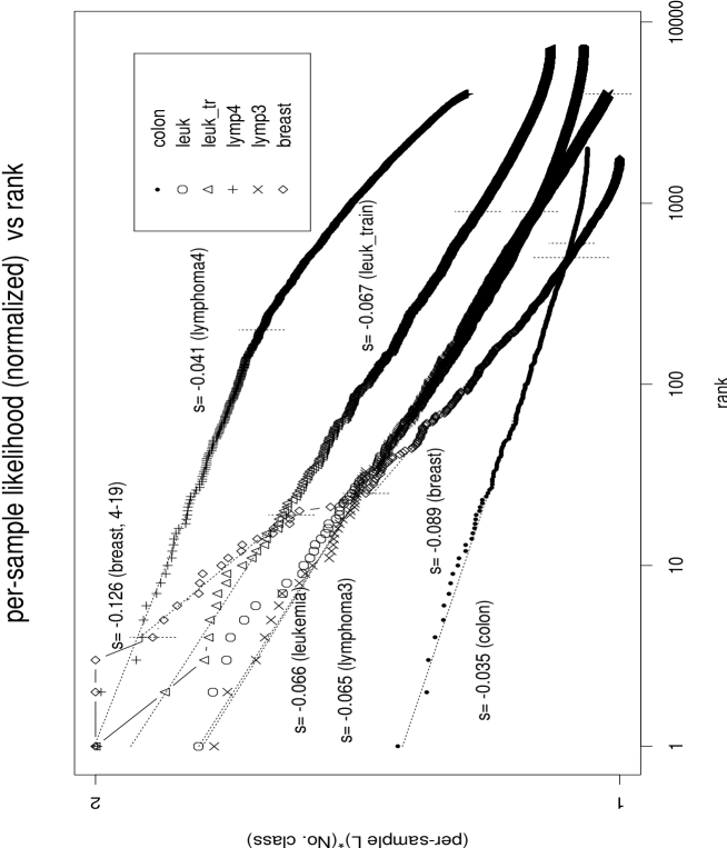
Figure 5: Normalized, per-sample maximum likelihood ($\hat{l}_{r}=\hat{L}_{r}^{1/N}/(1/C)$) where $C$ is the number of classes (e.g., $C=2$ for binomial logistic regression) for top genes vs. gene ranks, for all data sets. The corresponding $\hat{L}_{r}$ vs rank plots are in Figs. 1-4.

Fig.5 shows the Zipf’s plot of normalized per-sample likelihood $\hat{l}_{r}$ for all data sets analyzed so far. These curves can be compared in two ways. First, the performance of the top-ranking genes can be compared by their $\hat{l}_{r}$’s. It is clear from Fig.5 that for the leukemia data, the performance obtained from the training set is better than that obtained from the whole set, indicating a possible heterogeneity in the data set. The performance of the top genes for the breast cancer data set is better (in terms of classification) than that for the leukemia data set, which in turn is better than that for the colon cancer data set.

It is usually difficult to compare performance between a two-label classification and a multiple-label classification, because it depends on the base-line expectation. Two base-line expectations (called null models) were defined in [Li & Yang, 2001, Li, et al., 2001]: one is to randomly guess all classes with equal probability, and another is to guess the class by the proportion of samples with this class in the data set. In Fig.5, the first base-line expectation is used as the normalization factor. The performance of the 4-label classification relative to this base-line expectation for the lymphoma data is considered to be better than that of the 3-label classification, partly due to its low expectation.

Different data sets in Fig.5 can also be compared by the rate of falling of likelihood. The fall-off rate, as measured by the scaling exponent $\alpha$, ranges from 3 to 9 per 100 samples (i.e., $\alpha/N\approx 0.03-0.09$). It is interesting that scaling exponents obtained from the leukemia data (both the whole data set and the training set) and from the lymphoma data (two DLBCL subtypes plus normal) are almost identical (around 65 - 67 per 100 samples). The breast cancer data is different from other data sets for falling faster in the likelihood-rank plot.

7 Discussion

Results from Figs. 1-4 established that when microarray data is used to classify cancer tissues, the classification likelihood of individual genes follows a generalized form of Zipf’s law. The reason that these power-law functions in the Zipf’s plot do not have a scaling exponent equal to 1 is partly because exponent $\alpha$ in Eq.(5) depends on the sample size $N$. Besides the issue of the exponent value, the overall power-law trend is excellent: a perfect power-law function for all points in Fig.3 (3-label classification, in 3.5 decades), a partial power-law fitting in a range of 2.5 decades (Fig.1), 3 decades (Fig.2), and 2 decades (Fig.3, 4-label classification), respectively. The only poor fitting by a power-law function is Fig.4. The Zipf’s plot is flattern out for low-ranking genes in Figs. 1 and 2, while it drops off in Fig.3 (4-label classification). Which functional form is more generic for low-ranking genes is not clear, perhaps our results are sample-size sensitive.

Our Zipf’s plot can be compared to those obtained from biomolecular sequences. In [Gamow & Yc̆as, 1955], a Zipf’s plot for 20 amino acids usage in protein sequences was presented (in linear-linear scale). Redrawing their data in log-log scale does not show any power-law behavior (result not shown). Recently, it was claimed that oligonucleotide frequencies in DNA sequences follow Zipf’s law [Mantegna, et al., 1994]. This paper drew criticism on its strong claim concerning the connection between Zipf’s law and human language [Martindale & Konopka, 1995; Israeloff, et al., 1996, Bonhoeffer, et al., 1996a,1996b, Voss, 1996]: one of the best counter-examples is Zipf’s law in money-typing texts [Li, 1992]. Also, the paper did not show convincingly that the Zipf’s plot for oligonucleotide usage was better fitted by a power-law function [Martindale & Konopka, 1996]: the deviation from the power-law fitting function can be gradual and systematic, an indication that the power-law function is not the best choice of fitting function. Finally, the scaling exponent in the power-law fitting function in [Mantegna, et al., 1994] is much smaller than 1 [Li, 1996]. In comparison, our Zipf’s plots in Figs 1-5 are a much better example of a generalized form of Zipf’s law than those in [Gamow & Yc̆as, 1955] and [Mantegna, et al., 1994].

One may wonder whether the power-law behavior in Figs 1-5 can be derived by a simple random model. In [Gamow & Yc̆as, 1955], the Zipf’s plot of the frequency of amino acids usage was compared to a “random partition of a unit length” model. Suppose a unit interval is randomly partitioned into $p$ segments (e.g. $p=20$ for 20 amino acids). These segments are ranked by their size $L_{(1)}=max_{i}(L_{i}),L_{(2)}=max_{i}(L_{i}\in L-L_{(1)})\cdot L_{(p)}=min_{i}(L_{i})$, etc. If this random partition is repeated, the mean value of the ranked size can be shown to be [Gamow & Yc̆as, 1955]:

$$<L_{(r)}>=\frac{1}{p}\sum_{i=1}^{p+1-r}\frac{1}{p+1-i}\hskip 7.22743pt\mbox{ $r=1,2,\cdots p$}$$ (8)

Drawing $<L_{(r)}>$ from Eq.(8) versus rank $r$ shows that it is a straight line in linear(y)-log(x) plot, and not a straight line in either log-log or log(y)-linear(x) plots (results not shown). Actually this analytic result may not be applicable to our case, because we keep track of the performance of a given gene on all samples, whereas in Eq.(8) the longest interval (or any given ranking interval) is averaged over all random simulation. In any case, the power-law behavior in Fig.1-5 does not seem to be explainable by a simple random model.

We may ask whether Zipf’s plot has any practical application for microarray data analysis. In information retrieval [van Rijsbergen, 1975, Salton, 1988] and library/documentation science [Egghe & Rousseau, 1990], Zipf’s law is an important foundation that many applications are based upon. It is one of the “bibliometric laws” [White & McCain, 1989] concerning regularities in bibliographies, lists of authors, citation lists, etc. For the purpose of finding relevant, content-bearing words (“keywords”), common (highest-ranking) and rare (lowest-ranking) words should be avoided [Luhn, 1957,1958].

Do we have a similar situation where the highest-ranking genes may not be interesting for cancer classification? (Lowest-ranking genes are obviously not interesting.) Our ranking system is not really the same as for word usage, since a discrimination or classification ability has already been included in our definition, whereas it is not included in the word usage example. In this sense, our top ranking genes are in fact most efficient for the purpose of cancer classification. On the other hand, if one is more interested in subtle gene effects, not in the known main/dominant effect, it is perhaps useful to remove the well-known genes from the list and examine other genes in a future study. This idea was not tried in our previous analysis [Li & Yang, 2001, Li, et al., 2001].

In conclusion, a generalized form of Zipf’s law was observed in microarray data for the likelihood on cancer classification using single-gene logistic regression. We suspect that this power-law behavior is generic rather than an exception. A rank-likelihood plot (Zipf’s plot) can be a useful quantitative tool for discriminant microarray data analysis.

Acknowledgements: The author would like to thank Yaning Yang for discussion on the random partition of unit interval, Ronald Rousseau and Heting Chu for suggesting references on library sciences, Victoria Haghighi and Joanne Edington for help with the microarray data. The work was supported by NIH grants K01HG00024 and HG00008.

References

Agresti A (1996), An Introduction to Categorical Data Analysis (Wiley & Sons).

Alizadeh AA, Eisen MB, et al. (2000), “Distinct types of diffuse large B-cell lymphoma identified by gene expression profiling”, Nature, 403:503-511.

Alon U, Barkai N, Notterman DA, Gish K, Ybarra S, Mack D, Levine AJ (1999), “Broad patterns of gene expression revealed by clustering analysis of tumor and normal colon tissues probed by oligonucleotide arrays”, Proceedings of National Academy of Sciences, 96(12):6745-6750.

Bonhoeffer S, Herz AVM, Boerlijst MC, Nee S, Nowak MA, May RM (1996a) “Explaining ’linguistic features’ of noncoding DNA”, Science, 271(5245):14-15.

Bonhoeffer S, Herz AVM, Boerlijst MC, Nee S, Nowak MA, May RM (1996b), “No signs of hidden language in noncoding DNA” (letters), Physical Review Letters, 76(11):1977.

Breslow NE, Day NE (1980), Statistical Methods in Cancer Research. I - The Analysis of Case-Control Studies (International Agency for Research on Cancer, Lyon).

Burnham KP, Anderson DR (1998), Model Selection and Inference (Springer).

Chatzidimitriou-Dreismann CA, Streffer RMF, Larhammar D (1996), “Lack of biological significance in the ’linguistic features’ of noncoding DNA-a quantitative analysis”, Nucleic Acids Research, 24(9):1676-1681.

Chen YS, Leimkuhler FF (1987), “Analysis of Zipf’s law: an index approach”, Information Processing and Management, 23:71-182.

Crovella ME, Bestavros A (1997), “Self-similarity in world wide web traffic: evidence and possible causes”, IEEE/ACM Transactions on Networking, 5(6):835-846.

Edwards AWF (1972), Likelihood (Cambridge Univ Press).

Egghe L, Rousseau R (1990), Introduction to Informetrics: Quantitative Methods in Library, Documentation and Information Science (Elsevier).

Ekins R, Chu FW (1999), “Microarrays: their origin and applications”, Trends in Biotechmology, 17:217-218.

Fodor SP, Read JL, Pirrung MC, Stryer L, Lu AT, Solas D (1991), “Light-directed, spatially addressable parallel chemical synthesisLight-directed, spatially addressable parallel chemical synthesis”, Science, 251:767-773.

Gamow G, Yc̆as M (1955), “Statistical correlation of protein and ribonucleic acid composition”, Proceedings of National Academy of Sciences, 41(12):1011-1019.

Geisser S (1993), Predictive Inference: An Introduction (Chapman & Hall).

Golub TR, Sonim DK, Tamayo P, Huard C, Gassenbeek M, Mesirov JP, Coller H, Loh ML, Downing JR, Caligiuri MA, Bloomfield CD, Lander ES (1999), “Molecular classification of cancer: class discovery and class prediction by gene expression monitoring”, Science, 286:531-536.

IHGSC (International Human Genome Sequencing Consortium) (2001), “Initial sequencing and analysis of the human genome”, Nature, 409:860-921.

Israeloff NE, Kagalenko M, Chan K (1996), “Can Zipf distinguish language from noise in noncoding DNA?” (letters) Physical Review Letters, 76(11):1976.

Haines JL, Pericak-Vance MA (1998), eds. Approaches to Gene Mapping in Complex Human Diseases (Wiley-Liss).

Lauria F, Raspadori D, et al. (1994), “Increased expression of myeloid antigen markers in adult acute lymphoblastic leukemia patients: diagnostic and prognostic implications”, British Journal of Haematology, 87:286-292.

Li W (1992), “Random texts exhibit Zipf’s-law-like word frequency distribution”, IEEE Transactions on Information Theory, 38:1842-1845.

Li W (1996), “Comments on ’Bell curves and monkey languages’ ” (letters to the editor), Complexity, 1(6):6.

Li W, Yang Y (2001), “How many genes are needed for a discriminant microarray data analysis?”, Proceedings of the Critical Assessment of Microarray Data Analysis Workshop (CAMDA 2000).

Li W, Yang Y, Edington J, Haghighi F (2001), “Determining the number of genes needed for cancer classification using microarray data”, submitted.

Luhn HP (1957), “A statistical approach to mechanized encoding and search of literature information”, IBM Journal of Research and Development, 1:309-317.

Luhn HP (1958), “The automatic creation of literature abstract”, IBM Journal of Research and Development, 2:159-165.

Mantegna RN, Buldyrev SV, Goldberger AL, Havlin S, Peng CK, Simon M, Stanley HE (1994), “Linguistic features of noncoding DNA sequences”, Physical Review Letters, 73:3169-3172.

Martindale C, Konopka AK (1995), “Noncoding DNA, Zipf’s law, and language” (letters), Science, 268(5212):789.

Martindale C, Konopka AK (1996), “Oligonucleotide frequencies in DNA follow a Yule distribution”, Computers and Chemistry, 20:35-38.

Perou CM, Sorlie T, et al. (2000), “Molecular portraits of human breast tumors”, Nature, 406:747-752.

Raftery AE (1995), “Bayesian model selection in social research”, in Sociological Methodology, ed. PV Marsden (Blackwells), pages 185-195.

Salton G (1988), Automatic Text Processing: The Transformation, Analysis, and Retrieval of Information (Addison-Wesley).

Schena M, Shalon D, Davis RW, Brown PO (1995), “Quantitative monitoring of gene expression patterns with a complementary DNA microarray”, Science, 270:467-470.

Shalon D, Smith SJ, Brown PO (1996), “A DNA microarray system for analyzing complex DNA samples using two-color fluorescent probe hybridization”, Genome Research, 6:639-645.

Sornette D, Knopoff L, Kagan YY, Vanneste C (1996), “Rank-ordering statistics of extreme events: application to the distribution of large earthquakes”, Journal of Geophysical Research, 101(B6):13883-13894.

Southern EM (1996), “DNA chips: analysing sequence by hybridization to oligonucleotides on a large scale”, Trends in Genetics, 12:110-115.

van Rijsbergen CJ (1975), Information Retrieval (Butterworths).

Venter JC (2001), et al. “The sequence of the human genome”, Science, 291:1304-1351.

Voss RF (1996), “Linguistic features of noncoding DNA sequences - Comment” (letters), Physical Review Letters, 76(11):1978.

White HD, McCain KW (1989), “Bibliometrics”, Annual Review of Information Science and Technology, 24:119-186.

Zipf GF (1935), Psycho-Biology of Languages (Houghton-Mifflin)

Zipf GF (1949), Human Behavior and the Principle of Least Effort (Addison-Wesley).

Figure 1: Zipf’s plot for colon cancer and normal tissue classification: maximized likelihood of single-variable logistic regression (Eq.(3)) for the top performing genes vs their ranks (in log-log scale).

Figure 2: Zipf’s plot for leukemia subtype classification: maximized likelihood of single-variable logistic regression (Eq.(3)) for the top genes vs their ranks, in log-log scale. The upper line is obtained from the “training set” which contains 38 samples, and the lower line is from the “training plus testing set” which contains 72 samples.

Figure 3: Zipf’s plot for lymphoma subtypes classification: maximized likelihood of single-variable multinomial logistic regression (Eq.(6)) for top-ranking genes vs. their ranks, in log-log scale. The upper line is for the 3-class classification (GC-DLBCL, A-DLBCL, normal), and the lower line is for the 4-class situation (DLBCL, FL, CLL, normal).

Figure 4: Zipf’s plot for the breast cancer treatment effect: maximized likelihood of single-variable paired case-control logistic regression (Eq.(7)) for top genes vs. their rank (in log-log scale).