Quasilinearization Approach to Nonlinear Problems in Physics with Application to Nonlinear ODEs

Abstract

The general conditions under which the quadratic, uniform and monotonic convergence in the quasilinearization method of solving nonlinear ordinary differential equations could be proved are formulated and elaborated. The generalization of the proof to partial differential equations is straight forward. The method, whose mathematical basis in physics was discussed recently by one of the present authors (VBM), approximates the solution of a nonlinear differential equation by treating the nonlinear terms as a perturbation about the linear ones, and unlike perturbation theories is not based on the existence of some kind of a small parameter.

It is shown that the quasilinearization method gives excellent results when applied to different nonlinear ordinary differential equations in physics, such as the Blasius, Duffing, Lane-Emden and Thomas-Fermi equations. The first few quasilinear iterations already provide extremely accurate and numerically stable answers.

PACS numbers: 02.30.Mv, 04.25.Nx, 11.15.Tk

I Introduction

In a series of recent papers, [1, 2] the possibility of applying a very powerful approximation technique called the quasilinearization method (QLM) to physical problems has been discussed. The QLM is designed to confront the nonlinear aspects of physical processes. The method, whose iterations are constructed to yield rapid convergence and often monotonicity, was originally introduced forty years ago by Bellman and Kalaba [3, 4] as a generalization of the Newton-Raphson method [5, 6] to solve individual or systems of nonlinear ordinary and partial differential equations. Modern developments and applications of the QLM to different fields are given in a monograph [7].

However, the QLM was never systematically studied or extensively applied in physics, although references to it can be found in well known monographs [8, 9] dealing with the variable phase approach to potential scattering, as well as in a few scattered research papers [10, 11, 12, 13]. The reason for the sparse use of the QLM in Physics is that the convergence of the method has been proven only under rather restrictive conditions [3, 4], which generally are not fulfilled in physical applications. Recently, though, it was shown [1] by one of the present authors (VBM) that a different proof of the convergence can be provided which we will generalize and elaborate here so that the applicability of the method is extended to incorporate realistic physical conditions of forces defined on infinite intervals with possible singularities at certain points.

In the first paper of the series [1], the quasilinearization approach was applied to the nonlinear Calogero equation in a variable phase approach to quantum mechanics and the results were compared with those of perturbation theory and the exact solutions. It was found analytically and by examples that the $n$-th approximation of the QLM exactly sums $2^{n}-1$ terms of perturbation theory. In addition, a similar number of terms is reproduced approximately. The number of the exactly reproduced perturbation terms thus doubles with each subsequent QLM approximation, and reaches, for example, 127 terms in the 6-th QLM approximation, 8191 terms in the 12-th QLM approximation, and so on.

The computational approach in the work [1] was mostly analytical, and therefore one was able to compute only two to three QLM iterations, mainly for power potentials. Only in the case of the $1/r^{2}$ potential, could the calculation of QLM iterations be done analytically for any $n$.

The goal of the next work [2] was, by dropping the restriction of analytical computation, to calculate higher iterations as well as to extend the analysis to non-power potentials, in order to better assess the applicability of the method and of its numerical stability and the convergence pattern of the QLM iterations. It was shown that the first few iterations already provide very accurate and numerically stable answers for small and intermediate values of the coupling constant and that the number of iterations necessary to reach a given precision only moderately increases for larger values of the coupling. The method provided accurate and stable answers for any coupling strengths, including for super singular potentials for which each term of the perturbation theory diverges and the perturbation expansion does not exist even for a very small coupling.

The quasilinearization approach is applicable to a general nonlinear ordinary or partial $n$ -th order differential equation in $N$-dimensional space. In this paper, we consider the case of nonlinear ordinary differential equations in one variable which, unlike the nonlinear Calogero equation[8] considered in references[1, 2], contain not only quadratic nonlinear terms but various other forms of nonlinearity and not only a first, but also higher derivatives. Namely, we apply it to a panopoly of well-known and difficult nonlinear ordinary first, second and third order differential equations and show that again with just a small number of iterations one can obtained fast convergent and uniformly excellent and stable numerical results.

The paper is arranged as follows: in the second chapter we present the main features of the quasilinearization approach, while in the third chapter we consider, as a warm-up exercise, a simple first-order differential equation with a nonlinear $n$-th power term and compare its exact analytic solution with the perturbation theory and with the QLM iterations in order to demonstrate the main features of the quasilinearization approach. In the next four chapters, we apply our method to four well known nonlinear ordinary second and third order differential equations, namely to the Lane-Emden, Thomas-Fermi, Duffing, and Blasius equations, respectively. These equations have been extensively studied in the literature. For a sample of recent papers see refs. [15, 16, 17, 18, 19, 20, 21, 22] and references therein.

The results, convergence patterns, numerical stability, advantages of the method and its possible future applications are discussed in the final chapter.

II The quasilinearization method (QLM)

The aim of the quasilinearization method (QLM) of Bellman and Kalaba [3, 4, 7] based on the Newton-Raphson method [5, 6] is to solve a nonlinear $n$-th order ordinary or partial differential equation in $N$ dimensions as a limit of a sequence of linear differential equations. This goal is easily understandable since there is no useful technique for obtaining the general solution of a nonlinear equation in terms of a finite set of particular solutions, in contrast to a linear equation which can often be solved analytically or numerically in a convenient fashion using superposition. In addition, the QL sequence should be constructed to assure quadratic convergence and, if possible, monotonicity.

As we have mentioned in the Introduction, we will follow here the derivation outlined in ref. [1], which is not based, unlike the derivations in refs. [3, 4], on a smallness of the interval and on the boundness of the nonlinear term and its functional derivatives, the conditions which usually are not fulfilled in physical applications.

For simplicity, we limit our discussion to nonlinear ordinary differential equation in one variable on the interval $[0,b],$ which could be infinite:

$$\L^{(n)}u(x)=f(u(x),u^{(1)}(x),....u^{(n-1)}(x),x),\$$ (1)

with $n$ boundary conditions

$$g_{k}(u(0),u^{(1)}(0),....,u^{(n-1)}(0))=0,\;k=1,...l$$ (2)

and

$$g_{k}(u(b),u^{(1)}(b),....,u^{(n-1)}(b))=0,\;k=l+1,...,n.$$ (3)

Here $L^{(n)}$ is linear $n$-th order ordinary differential operator and $f$ and $g_{1},g_{2},.....,g_{n}$ are nonlinear functions of $u(x)$ and its $n-1$ derivatives $u^{(s)}(x),s=1,...n-1$. The more general case of partial differential equations in N-dimensional space could be considered in exactly the same fashion by changing the definition of $L^{(n)}$ to be a linear $n$-th order differential operator in partial derivatives and $x$ to be an N-dimensional coordinate array.

The QLM prescription [1, 3, 4] determines the $r+1$-th iterative approximation $u_{r+1}(x)$ to the solution of Eq. (1) as a solution of the linear differential equation

$$L^{(n)}u_{r+1}(x)=f(u_{r}(x),u^{(1)}_{r}(x),.....,u^{(n-1)}_{r}(x),x)$$ (4)

$$+\sum_{s=0}^{n-1}\bigl{(}u^{(s)}_{r+1}(x)-u^{(s)}_{r}(x)\bigr{)}\,f_{u^{(s)}}(u_{r}(x),u^{(1)}_{r}(x),.....,u^{(n-1)}_{r}(x),x),$$ (5)

where $u^{(0)}_{r}(x)=u_{r}(x)$, with linearized two-point boundary conditions

$$\sum_{s=0}^{n-1}\bigl{(}u^{(s)}_{r+1}(0)-u^{(s)}_{r}(0)\bigr{)}\,g_{ku^{(s)}}(u_{r}(0),u^{(1)}_{r}(0),.....,u^{(n-1)}_{r}(0),0)=0,\;\ k=1,...l$$ (6)

and

$$\sum_{s=0}^{n-1}\bigl{(}u^{(s)}_{r+1}(b)-u^{(s)}_{r}(b)\bigr{)}\,g_{ku^{(s)}}(u_{r}(b),u^{(1)}_{r}(b),.....,u^{(n-1)}_{r}(b),b)=0,\;\ k=l+1,...,n.$$ (7)

Here the functions $f_{u^{(s)}}={\partial{f}}/{\partial{u^{(s)}}}$ and $g_{ku^{(s)}}={\partial{g_{k}}}/{\partial{u^{(s)}}},\ s=0,1,...,n-1$ are functional derivatives of the functionals $f(u(x),u^{(1)}(x),....u^{(n-1)}(x),x)$ and $g_{k}(u(x),u^{(1)}(x),....u^{(n-1)}(x),x)$, respectively. .

The zeroth approximation $u_{0}(x)$ is chosen from mathematical or physical considerations.

To prove that the above procedure yields a quadratic and often monotonic convergence to the solution of Eq. 1 with the boundary conditions 2 and 3, we follow reference [1] and consider a differential equation for the difference $\delta u_{r+1}(x)\equiv u_{r+1}(x)-u_{r}(x)$ between two subsequent iterations:

$$L^{(n)}\delta u_{r+1}(x) = [f(u_{r}(x),u^{(1)}_{r}(x),.....,u^{(n-1)}_{r}(x),x)-f(u_{r-1}(x),u^{(1)}_{r-1}(x),.....,u^{(n-1)}_{r-1}(x),x)]$$ (8)

$$+ \sum_{s=0}^{n-1}[\delta u^{(s)}_{r+1}(x)\,f_{u^{(s)}}(u_{r}(x),u^{(1)}_{r}(x),.....,u^{(n-1)}_{r}(x),x)$$ (9)

$$- \delta u^{(s)}_{r}(x)\,f_{u^{(s)}}{u_{(}r-1}(x),u^{(1)}_{r-1}(x),.....,u^{(n-1)}_{r-1}(x),x)].$$ (10)

The boundary conditions are similarly given by the difference of Eqs. 6 and 7 for two subsequent iterations:

$$\sum_{s=0}^{n-1}[\delta u^{(s)}_{r+1}(0)\ g_{ku^{(s)}}(u_{r}(0),u^{(1)}_{r}(0),.....,u^{(n-1)}_{r}(0),0)$$ (11)

$$-\delta u^{(s)}_{r}(0)\ g_{ku^{(s)}}(u_{r-1}(0),u^{(1)}_{r-1}(0),.....,u^{(n-1)}_{r-1}(0),0)] = 0,$$ (12)

$$k = 1,...l$$ (13)

and

$$\sum_{s=0}^{n-1}[\delta u^{(s)}_{r+1}(b)\ g_{ku^{(s)}}(u_{r}(b),u^{(1)}_{r}(b),.....,u^{(n-1)}_{r}(b),b)$$ (14)

$$-\delta u^{(s)}_{r}(b)\ g_{ku^{(s)}}(u_{r-1}(b),u^{(1)}_{r-1}(b),.....,u^{(n-1)}_{r-1}(b),b)] = 0,$$ (15)

$$k = l+1,...n.$$ (16)

In view of the mean value theorem[14]

$$f(u_{r}(x),u^{(1)}_{r}(x),.....,u^{(n-1)}_{r}(x),x)-f(u_{r-1}(x),u^{(1)}_{r-1}(x),.....,u^{(n-1)}_{r-1}(x),x)=$$ (17)

$$\sum_{s=0}^{n-1}\delta u^{(s)}_{r}(x)\ f_{u^{(s)}}(u_{r-1}(x),u^{(1)}_{r-1}(x),.....,u^{(n-1)}_{r-1}(x),x)+$$ (18)

$$\frac{1}{2}\sum_{s,t=0}^{n-1}\delta u^{(s)}_{r}(x)\,\delta u^{(t)}_{r}(x)\ f_{u^{(s)}u^{(t)}}(\bar{u}_{r-1}(x),\bar{u}^{(1)}_{r-1}(x),.....,\bar{u}^{(n-1)}_{r-1}(x),x),$$ (19)

where $\bar{u}^{(s)}_{r-1}(x)$ lies between $u^{(s)}_{r}(x)$ and $u^{(s)}_{r-1}(x)$. Now Eq. 10 can be written as

$$L^{(n)}\delta u_{r+1}(x)-\sum_{s=0}^{n-1}\delta u^{(s)}_{r+1}(x)\,f_{u^{(s)}}(u_{r}(x),u^{(1)}_{r}(x),.....,u^{(n-1)}_{r}(x),x)=$$ (20)

$$\frac{1}{2}\sum_{s,t=0}^{n-1}\delta u^{(s)}_{r}(x)\delta u^{(t)}_{r}(x)\,f_{u^{(s)}u^{(t)}}(\bar{u}_{r-1}(x),\bar{u}^{(1)}_{r-1}(x),.....,\bar{u}^{(n-1)}_{r-1}(x),x).$$ (21)

Denoting $G_{r}^{(n)}(x,y)$ as the Greens function, which is the inverse of the following differential operator and incorporates linearized boundary conditions 6 and 7,

$$\tilde{L}^{(n)}=L^{(n)}-\sum_{s=0}^{n-1}f_{u^{(s)}}(u_{r}(x),u^{(1)}_{r}(x),.....,u^{(n-1)}_{r}(x),x)\ \frac{d^{s}}{{dx}^{s}}\;,$$ (22)

one can express the solution for the difference function $\delta u_{r+1}$ as

$$\delta u_{r+1}(x)=$$ (23)

$$\frac{1}{2}\int_{0}^{b}G_{r}^{(n)}(x,y) \sum_{s,t=0}^{n-1}\delta u^{(s)}_{r}(y)\delta u^{(t)}_{r}(y)\,f_{u^{(s)}u^{(t)}}(\bar{u}_{r-1}(y),\bar{u}^{(1)}_{r-1}(y),.....,\bar{u}^{(n-1)}_{r-1}(y),y)\,dy.$$ (24)

The functions $\delta u^{(s)}_{r}(y)\delta u^{(t)}_{r}(y)$ could be taken outside of the sign of the integral at some point $y=\bar{x}$ belonging to the interval, so one obtains

$$\delta u_{r+1}(x)=\frac{1}{2}\sum_{s,t=0}^{n-1}\delta u^{(s)}_{r}(\bar{x})\delta u^{(t)}_{r}(\bar{x})M_{st}(x).$$ (25)

where $M_{sr}(x)$ equals

$$M_{st}(x)=\int_{0}^{b}G_{r}^{(n)}(x,y)f_{u^{(s)}u^{(t)}}(\bar{u}_{r-1}(y),\bar{u}^{(1)}_{r-1}(y),.....,\bar{u}^{(n-1)}_{r-1}(y),y)dy$$ (26)

If $M_{st}(x)$ is a strictly positive (negative) matrix for all $x$ in the interval, then $\delta u_{r+1}(x)$ will be positive (negative), and the monotonic convergence from below (above) results.

Obviously, from Eq. 24 follows

$$|\delta u_{r+1}(x)|\leq\it{k_{r}}(x)||\delta u_{r}||^{2}$$ (27)

where $\it{k}_{r}$ is given by

$$\it{k_{r}}(x)=\frac{1}{2} \int_{0}^{b}|G_{r}^{(n)}(x,y)|\sum_{s,t=0}^{n-1}|f_{u^{(s)}u^{(t)}}(\bar{u}_{r-1}(y),\bar{u}^{(1)}_{r-1}(y),.....,\bar{u}^{(n-1)}_{r-1}(y),y)|dy$$ (28)

and $||\delta u_{r}||$ is a maximal value of any of $|\delta\bar{u}^{(s)}_{r}|$ on the interval (0,b).

Since Eq. 27 is correct for any $x$ on the interval (0,b), it is correct also for some $x=\bar{x}$ where $|\delta u_{r+1}(x)|$ reaches its maximum value $||\delta u_{r+1}||$. One therefore has

$$||\delta u_{r+1}|||\leq\it{k_{r}}(\bar{x})||\delta u_{r}||^{2}$$ (29)

Assuming the boundness of the integrand in expression 28, that is the existence of the bounding function $F(x)$ such that integrand at $x=\bar{x}$ and at any $y$ is less or equal to $F(y)$, one finally has

$$||\delta u_{r+1}|||\leq\it{k}||\delta u_{r}||^{2}\;,$$ (30)

where

$$\it{k}=\int_{0}^{b}F(x)dx\;.$$ (31)

The linearized boundary conditions 6 and 7 are obtained from exact boundary conditions 2 and 3 by using the mean value theorem Eq. 19 and neglecting the quadratic terms, so that the error in using linearized boundary conditions vis-a-vis the exact ones is quadratic in the difference between the exact and linearized solutions. The maximum difference between boundary conditions 6 and 7 corresponding to two subsequent quasilinear iterations is therefore quadratic in $||\delta u_{r}||$. In view of this result and of Eq. 30, the difference between the subsequent iterative solutions of Eq.5 with boundary conditions 6 and 7 decreases quadratically with each iteration. In a similar way, one can show [1] that the difference $\Delta u_{r+1}(x)=u(x)-u_{r}(x)$ between the exact solution and the $r$-th iteration is decreasing quadratically as well:

$$||\Delta u_{r+1}|||\leq\it{k}||\Delta u_{r}||^{2}\;.$$ (32)

A simple induction of Eq. 30 shows [4] that ${\delta}u_{n+1}(x)$ for an arbitrary $l<r$ satisfies the inequality

$${\parallel}\delta u_{r+1}{\parallel}\leq(\it{k}{\parallel}\delta u_{l+1}{\parallel})^{2^{r-l}}/\it{k},$$ (33)

or, for $l=0$, we can relate the $n+1$ th order result to the 1st iterate by

$${\parallel}\delta u_{n+1}{\parallel}\leq((\it{k}{\parallel}\delta u_{1}{\parallel})^{2^{n}}/k.$$ (34)

The convergence depends therefore on the quantity $q_{1}=\it{k}{\parallel}{u_{1}-u_{0}}{\parallel}$, where, as we have mentioned earlier, the zeroth iteration $u_{0}(x)$ is chosen from physical and mathematical considerations. Usually it is advantageous (see discussion below) that $u_{0}(x)$ would satisfy at least one of the boundary conditions. From Eq. (33) it follows, however, that for convergence it is sufficient that just one of the quantities $q_{m}=\it{k}{\parallel}\delta u_{m}{\parallel}$ is small enough. Consequently, one can always hope [4] that even if the first convergent coefficient $q_{1}$ is large, a well chosen initial approximation $u_{0}$ results in the smallness of at least one of the convergence coefficients $q_{m},\ m>1$, which then enables a rapid convergence of the iteration series for $r>m$. It is important to stress that in view of the quadratic convergence of the QLM method, the difference $||\Delta u_{r+1}||$ between the exact solution and the QLM iteration always converges to zero if the difference $\delta u_{r+1}(x)$ between two subsequent QLM iterations becomes infinitesimally small.

Indeed, if $\delta u_{r}(x)$ is close to zero, it means, since $\delta u_{r+1}(x)=\Delta u_{r}(x)-\Delta u_{r+1}(x)$ that $\Delta u_{r}(x)=\Delta u_{r+1}(x)$ or $Q_{r}=Q_{r+1}$ where $Q_{r}=\it{k}||\Delta u_{r}||$. When one assumes the possibility that $Q_{r}$ and $Q_{r+1}$ could be not small, one could conclude that the iteration process “stagnates”, which means convergence to the wrong answer or no convergence at all.

However, such a conclusion is wrong since Eq. 32, which can be written as $Q_{r+1}\leq Q^{2}_{r}$, for $Q_{r}\leq 1$ (this last inequality, starting from some r is a necessary condition of the convergence) could be not satisfied unless both $||Q_{r+1}||$ and $||Q_{r}||$ equal to zero. This proves that stagnation of the iteration process is impossible and convergence of $||\delta u_{r+1}||$ to zero automatically leads to convergence of the QLM iteration sequence to the exact solution. Hence the QLM assures not only convergence, but also convergence to the correct solution.

Another corollary of this iteration process is that if the solution and its derivatives are continuous functions of $x$, the convergence of the QLM in the whole region will follow. Indeed, even if the zero iteration $u_{0}(x)$ is chosen not to satisfy the boundary conditions, the next iteration $u_{1}(x)$, being a solution of a linear equation with linearized boundary conditions 6 and 7, will automatically satisfy the exact boundary conditions 2 and 3, at least up to the second order in difference $\delta u_{1}$ at the boundaries. This means that the difference between the exact and first QLM iterations at some intervals near the boundaries will be small, so that the QLM iterations in this interval would converge. Because the subsequent values of $\it{k}\,\delta u_{m}(x),m>2$ became much smaller for this interval, in view of assumed continuity of the solution and its derivatives these differences will also be small at the neighboring intervals. The subsequent iterations will extend the convergence to the next neighboring intervals and so on, until the convergence in the whole region will be reached. The predicted trend is therefore that the QLM yields rapid convergence starting at the regions where the boundary conditions are imposed and then spreading from there to all other regions.

An additional important corollary is that, in view of Eq. 33, once the quasilinear iteration sequence starts to converge, it will continue to do so, unlike the perturbation expansion, which is often given by an asymptotic series and therefore converges only up to a certain order and diverges thereafter.

Based on this summary of the QLM, one can deduce the following important features of the quasilinearization method:

• The method approximates the solution of nonlinear differential equations by treating the nonlinear terms as a perturbation about the linear ones, and is not based, unlike perturbation theories, on the existence of some kind of small parameter.

• The iterations converge uniformly and quadratically to the exact solution. In case of matrix $M_{st}$ in Eq. 26 being strictly positive (negative) for all $x$ in the interval, the convergence is also monotonic from below (above).

• For rapid convergence it suffices that an initial guess for the zeroth iteration is sufficiently good to ensure the smallness of just one of the quantities $q_{r}=\it{k}{\parallel}u_{r+1}-u_{r}{\parallel}$. If the solution and its derivatives are continuous, convergence follows from the fact that starting from the first iteration, all QLM iterations automatically satisfy the quasilinearized boundary conditions 6 and 7. The convergence is extremely fast: if, for example, $q_{1}$ is of the order of $\frac{1}{3}$, only 4 iterations are necessary to reach the accuracy of 8 digits, since $(\frac{1}{3})^{2^{n}}$ is of the order of $(\frac{1}{10})^{2^{n-1}}$.

• Convergence of $||\delta u_{r+1}||$ to zero automatically leads to convergence of the QLM iteration sequence to the exact solution.

• Once the quasilinear iteration sequence at some interval starts to converge, it will always continue to do so. Unlike an asymptotic perturbation series, the quasilinearization method yield the required precision once a successful initial guess generates convergence after a few steps.

III Analytically solvable example: comparison of quasilinearization approach with exact solution and with perturbation theory.

In order to investigate the applicability of the quasilinearization method and its convergence and numerical stability, let us start from a simple example of an analytically solvable nonlinear ordinary differential equation suggested in ref. [22]:

$$u^{\prime}(r)=-g\ u^{n}(r),\ \ \ u(0)=1,$$ (35)

where the boundary condition at $r=0$ is also given and ^′ means differentiation in variable $r$. The exact solution to this problem is

$$u(r)=(1+(n-1)\,g\,r)^{-\frac{1}{n-1}}$$ (36)

Since

$$(1+x)^{q}=\sum_{0}^{\infty}\frac{\Gamma(q+1)}{m!\Gamma(q+1-m)}\ x^{m},$$ (37)

the expansion of the solution 36 in powers of $g$ is given by

$$u(r)=\sum_{0}^{\infty}\frac{\Gamma(\frac{n-2}{n-1})(g(n-1))^{m}}{m!\Gamma(\frac{n-2}{n-1}-m)}\;r^{m}$$ (38)

The convergence radius of the series 38 is $R=1/(g\,(n-1)),$ which is inversely proportional to the extent $n-1$ of the nonlinearity and to the value $g$ of the perturbation parameter.

Now consider the quasilinearization approach to this equation, taking, for example, $g=1$ and $n=6.$ Here we consider Eq. 35 with a rather strong degree of nonlinearity. In this case, one can expect the convergence of the perturbation expansion only up to $r\leq\ R=\frac{1}{5}$.

The QLM procedure in the case where the nonlinear term depends only on the solution itself and not on its derivatives reduces to setting $u_{k+1}^{\prime}(r)=f(u_{k})+(u_{k+1}(r)-u_{k}(r))\ f_{u}(u_{k})$. Here $f=-g\;u^{n}(r)$ while its functional derivative $f_{u}$ equals to $-g\ nu^{n-1}(r)$. The quasilinearized equation 5 for the $(k+1)$-th iteration for this case has therefore the following form:

$$u_{k+1}^{\prime}(r)+ng\,u_{k}^{n-1}(r)\,u_{k+1}(r)=(n-1)\,g\,u_{k}^{n}(r),\ \ \ \ u_{k+1}(0)=1\;,$$ (39)

where $u_{k}(r)$ is a previous iteration which is considered to be a known function. Let us choose as a zero iteration $u_{0}(r)\equiv 1$ which satisfies the boundary condition $u_{0}(0)=1$.

The results of our QLM calculations with Eq. 39 are presented in Fig. 1 which displays the exact solution for the case of $n=6$ and $g=1,$ together with the first four QLM iterations. Convergence to the exact solution in Fig. 1 is monotonic from above as it should be as discussed in Section II and in Refs.[1, 3, 4] due to fact that the second functional derivative $-n(n-1)u^{n-2}(x)$ of the left-hand side of Eq.35 for even $n$ is strictly negative. The convergence starts at the boundary, exactly as expected from the discussion in section II, and expands with each iteration to larger values of the variable $r$. The difference between the exact solution and the sixth QLM iteration for all r in the range between zero and five where our calculations were performed is less than $10^{-6}.$ Note that the QLM yields a solution beyond the convergence radius limit on the series solution of $1/5.$

IV Lane-Emden equation

The Lane-Emden equation

$$y^{\prime\prime}(r)+\frac{2}{r}\;y^{\prime}(r)+y^{n}(r)=0,\ \ \ \ y(0)=1,\;y^{\prime}(0)=0$$ (40)

describes a variety of phenomena in theoretical physics and astrophysics, including aspects of stellar structure, the thermal history of a spherical cloud of gas, isothermal gas spheres, and thermionic currents, see ref. [17] and references therein. The parameter $n$ defines an equation of state with its physically interesting range being $0\leq n\leq 5$. The equation also appears in other contexts, e.g., in case of radiatively cooling, self gravitating gas clouds, in the mean-field treatment of a phase transition in critical absorption or in the modeling of clusters of galaxies. For $n=0,1$ and $5$ the equation can be solved analytically. Setting $y=\frac{u}{r}$ transforms the equation to a more convenient form without a first derivative:

$$u^{\prime\prime}(r)+\frac{u^{n}(r)}{r^{n-1}}=0,\;u(0)=0,\;u^{\prime}(0)=1.$$ (41)

Let us consider this nonlinear equation for the physically interesting and analytically nonsolvable case of $n=4$. The quasilinearized form of equation 41 is

$$u^{\prime\prime}_{k+1}(r)+n{\frac{u^{n-1}_{k}(r)}{r^{n-1}}}\;u_{k+1}(r)=\frac{n-1}{r^{n-1}}\;u^{n}_{k}(r),\;u_{k+1}(0)=0,\;u^{\prime}_{k+1}(0)=1.$$ (42)

The simplest initial guess, satisfying the boundary conditions will be $u_{0}(r)=r.$ Comparison of the quasilinear solutions corresponding to the first five iterations with the numerically computed exact solution are given in Fig. 2. The figure shows that the convergence to the exact solution is very fast. It starts, as in the example of the previous section, at the left boundary and spreads with each iteration to larger values of $r$ as expected from the discussion in section II. The difference between the exact solution and the eighth QLM iteration for all $r$ in the range between zero and ten, where our calculations were performed, is less than $10^{-11}$ .

V Thomas-Fermi equation

The Thomas-Fermi equation [23, 24]

$$\sqrt{x}\ u^{\prime\prime}(x)=u^{\frac{3}{2}}(x),\ \ \ \ u(0)=1,\;u(\infty)=0,$$ (43)

is an equation for the electron density around the nucleus of the atom. The left hand side of the above equation equals zero for $u<0.$ The Thomas-Fermi equation is also very useful for calculating form-factors and for obtaining effective potentials which can be used as initial trial potentials in self-consistent field calculations.. It is also applicable to the study of nucleons in nuclei and electrons in metal. It is long known (see [25] and references therein) that solution of this equation is very sensitive to a value of the first derivative at zero which insures smooth and monotonic decay from $u(0)=1$ to $u(\infty)=0$ as demanded by boundary conditions. By contrast, the computation is much simpler for the quasilinearized version of this equation. The QLM procedure in this case reduces to setting $u_{k+1}^{\prime\prime}(r)=f(u_{k})+(u_{k+1}(r)-u_{k}(r))f_{u}(u_{k})$, where $f=\frac{u^{3/2}(r)}{\sqrt{x}}$ and the functional derivative is $f_{u}=(3/2)\frac{u^{1/2}}{\sqrt{x}}$, so that the QLM equation has a form:

$$\sqrt{x}\;u_{k+1}^{\prime\prime}(x)-\frac{3}{2}\;u_{k}^{\frac{1}{2}}(x)\;u_{k+1}(x)=-\frac{1}{2}\;u_{k}^{\frac{3}{2}}(x),\;\;u_{k+1}(0)=1,\;\;u_{k+1}(\infty)=0,$$ (44)

which is easily solved by specifying directly the boundary condition at infinity without searching first for the proper value of the first derivative. The initial guess, satisfying the boundary condition at zero was chosen to be $u_{0}(x)\equiv 1$. The results of QLM calculations with Eq. 44 are presented in Fig. 3 which displays the exact solution together with the first four QLM iterations. The convergence starts at the boundaries, exactly as expected from the discussion in section II, and expands with each iteration to a wider range of values of the variable $x$. The difference between the exact solution and the eighth QLM iteration for all $x$ in the range between zero and forty where our calculations were performed is less than $10^{-7}.$

VI Classical anharmonic oscillator

The classical anharmonic oscillator satisfies the nonlinear second-order Duffing equation

$$\ddot{u}(t)+u(t)+g\ u^{3}(t)=0\ .$$ (45)

The typical initial conditions are

$$u(0)=1,\;\;\dot{u}(0)=0.$$ (46)

The solution oscillates strongly and thus is more difficult to approximate. It is, for example, well known [22] that the usual perturbative solution is valid only for times $t$ small compared with $\frac{1}{g}$, so that for larger $g$ the perturbative solution is adequate only on a small time interval. In contrast, the quasilinearization approach gives solution in the whole region also for large $g$-values.

The quasilinearized equation is

$$\ddot{u}_{k+1}(t)+(1+3\ g\ u^{2}_{k}(t))u_{k+1}(t)-2\ g\ u_{k}^{3}(t)=0,\ \ \ u_{k+1}(0)=1,\;\;\dot{u}_{k+1}(0)=0.$$ (47)

The results of QLM calculations with Eq. 47 for $g=3$ are presented in Figs. 4 and 5. Fig. 4 displays the exact solution together with the QLM solutions for the first, second and fourth iterations while Fig. 5 shows comparison of exact solution with sixth, seventh and eighth QLM iterations. Again, the convergence starts at the left boundary as expected from the discussion in section II, and expands with each iteration to larger values of the variable $t$. The difference between the exact solution and the eleventh QLM iteration for all t in the range between zero and seven where our calculations were performed is less than $10^{-10}$ .

VII Blasius equation

A third order nonlinear Blasius equation

$$u^{\prime\prime\prime}(x)+u^{\prime\prime}(x)u(x)=0,\ \ \ u(0)=u^{\prime}(0)=0\;\;,u^{\prime}(\infty)=1$$ (48)

describes the velocity profile of the fluid in the boundary layer. The QLM procedure in this case is given by $u_{k+1}^{\prime\prime\prime}(x)=f(u_{k},u_{k}^{\prime\prime})+(u_{k+1}-u_{k})f_{u}(u_{k},u_{k}^{\prime\prime})+(u_{k+1}^{\prime\prime}-u_{k}^{\prime\prime})f_{u^{\prime\prime}}(u_{k},u_{k}^{\prime\prime})$, where $f(u,u^{\prime})=-u^{\prime\prime}u$, $f_{u}(u,u^{\prime})=-u^{\prime\prime}$ and $f_{u^{\prime\prime}}(u,u^{\prime})=-u$. The quasilinearized version of the Blasius equation thus has a form

$$u_{k+1}^{\prime\prime\prime}(x)+u_{k}(x)u_{k+1}^{\prime\prime}(x)+u_{k+1}(x)u_{k}^{\prime\prime}(x)-u_{k}(x)u_{k}^{\prime\prime}(x)=0,$$ (49)

$$\;\;u_{k+1}(0)=u_{k+1}^{\prime}(0)=0\;\;,u_{k+1}^{\prime}(\infty)=1.$$ (50)

The initial guess, satisfying the boundary condition for the derivative at zero was chosen to be $u_{0}(x)\equiv 1$. The results of QLM calculations with Eq. 50 are presented in Fig. 6 which displays the exact solution together with the first QLM iteration. The convergence starts at the left boundary as follows from the discussion in section II, and expands with each iteration to larger values of the variable $x$. The difference between the exact solution and the fifth QLM iteration for all $x$ in the range between zero and ten where our calculations were performed is less than $10^{-11}$ .

VIII Conclusion

Summing up, we formulated here the conditions under which the quadratic, uniform and often monotonic convergence of the quasilinearization method are valid.

We have followed here the derivation outlined in ref. [1], which is not based, unlike the derivations in refs. [3, 4], on a smallness of the interval and on the boundness of the nonlinear term and its functional derivatives, the conditions which usually are not fulfilled in physical applications.

In order to analyze and highlight the power and features of the quasilinearization method (QLM), in this work we have also made numerical computations on different ordinary second and third order nonlinear differential equations, applied in physics, such as the Blasius, Duffing, Lane-Emden and Thomas-Fermi equations and have compared the results obtained by the quasilinearization method with the exact solutions. Although all our examples deal only with linear boundary conditions, the nonlinear boundary conditions can be handled readily after their quasilinearization as explained in Section II.

In all the examples considered in the paper the simplest initial guess was enough to produce a quadratic convergence. However, as it is well known for the Newton method on which quasilinearization method is based that the divergence could occur if the initial guess is too bad. In this case the modification of QLM based on the damped Newton method with relaxation factor /cite CB,RR may help. The price of such modification would be, like in the damped Newton method only linear convergence instead of the quadratic one.

Our conclusions are as follows:

The QLM treats nonlinear terms by a series of nonperturbative iterations and is not based on the existence of some kind of small parameter. At every iterative stage, the differential operator changes significantly to account for the nonlinearity, which is the major way that the QLM differs from other approximative techniques. As a result, as we see in all our examples, the QLM is able to handle large values of the coupling constant and any degree of the nonlinearity, unlike perturbation theory. Thus the QLM provides extremely accurate and numerically stable answers for a wide range of nonlinear physics problems. The QLM is also very easy to apply.

In view of all this, since most equations of physics, from classical mechanics to quantum field theory, are either not linear or could be transformed into a nonlinear form, the quasilinearization method appears to be extremely useful and in many cases more advantageous than the perturbation theory or its different modifications, like expansion in inverse powers of the coupling constant, the ${1}/{N}$ expansion, etc.

FIGURE CAPTIONS

FIG. 1. Convergence of QLM iterations for the analytic example of section III and comparison with the exact solution. Thin solid, dot-dashed, short-dashed and dotted curves correspond to the first, second, third and fourth QLM iteration respectively, while the thick solid curve displays the exact solution. The convergence is monotonic from above as it should be according to the discussion in the text. The difference between the exact solution and the sixth QLM iteration for all r in the figure is less than $10^{-6}$.

FIG. 2. Convergence of QLM iterations for the Lane-Emden equation and comparison with the numerically obtained exact solution. Thin solid, dot-dashed, short-dashed, long-dashed and dotted curves correspond to the first, second, third, fourth and fifth QLM iteration, respectively, while the thick solid curve displays the exact solution. The difference between the exact solution and the eighth QLM iteration for all r in the figure is less than $10^{-11}$

FIG. 3. Convergence of QLM iterations for the Thomas-Fermi equation and comparison with the numerically obtained exact solution. Thin solid, dot-dashed, short-dashed and dotted curves correspond to the first, second, third and fourth QLM iteration, respectively, while the thick solid curve displays the exact solution. The difference between the exact solution and the eighth QLM iteration for all x in the figure is less than $10^{-7}$ .

FIG. 4. Convergence of the first few QLM iterations for the Duffing equation and comparison with the numerically obtained exact solution. The dotted curves on three consecutive graphs correspond to the first, second and fourth QLM iteration respectively, while the solid curve displays the exact solution.

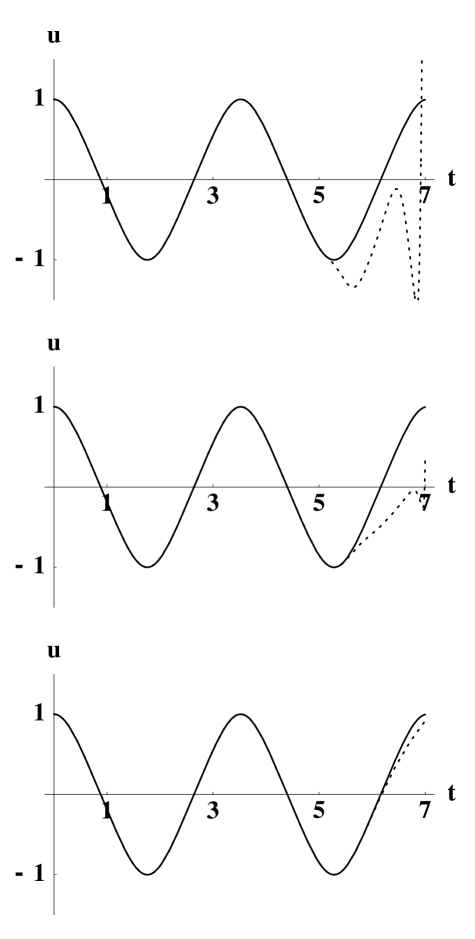
FIG. 5. Convergence of the higher QLM iterations for the Duffing equation and comparison with the numerically obtained exact solution. The dotted curves on the three consecutive graphs correspond to the sixth, seventh and eighth QLM iteration respectively, while the solid curve displays the exact solution. The difference between the exact solution and the eighth QLM iteration for all t in the figure is less than $10^{-10}$ .

FIG. 6. Comparison of the first QLM iteration for the Blasius equation with the numerically obtained exact solution. The difference between the exact solution and the fifth QLM iteration for all x in the figure is less than $10^{-10}$ .

FIG. 1.: Convergence of QLM iterations for the analytic example of section III and comparison with the exact solution. Thin solid, dot-dashed, short-dashed and dotted curves correspond to the first, second, third and fourth QLM iteration respectively, while the thick solid curve displays the exact solution. The convergence is monotonic from above as it should be according to the discussion in the text. The difference between the exact solution and the sixth QLM iteration for all r in the figure is less than $10^{-6}$.

FIG. 2.: Convergence of QLM iterations for the Lane-Emden equation and comparison with the numerically obtained exact solution. Thin solid, dot-dashed, short-dashed, long-dashed and dotted curves correspond to the first, second, third, fourth and fifth QLM iteration, respectively, while the thick solid curve displays the exact solution. The difference between the exact solution and the eighth QLM iteration for all r in the figure is less than $10^{-11}$ .

FIG. 3.: Convergence of QLM iterations for the Thomas-Fermi equation and comparison with the numerically obtained exact solution. Thin solid, dot-dashed, short-dashed and dotted curves correspond to the first, second, third and fourth QLM iteration, respectively, while the thick solid curve displays the exact solution. The difference between the exact solution and the eighth QLM iteration for all x in the figure is less than $10^{-7}$ .

FIG. 4.: Convergence of the first few QLM iterations for the Duffing equation and comparison with the numerically obtained exact solution. The dotted curves on three consecutive graphs correspond to the first, second and fourth QLM iteration respectively, while the solid curve displays the exact solution.

FIG. 5.: Convergence of the higher QLM iterations for the Duffing equation and comparison with the numerically obtained exact solution. The dotted curves on the three consecutive graphs correspond to the sixth, seventh and eighth QLM iteration respectively, while the solid curve displays the exact solution. The difference between the exact solution and the eighth QLM iteration for all t in the figure is less than $10^{-10}$ .

FIG. 6.: Comparison of the first QLM iteration for the Blasius equation with the numerically obtained exact solution. The difference between the exact solution and the fifth QLM iteration for all x in the figure is less than $10^{-10}$ .